碩士論文
Graduate Institute of Electronics Engineering College of Electrical Engineering & Computer Science
National Taiwan University Master thesis
雙向通道網路晶片之模塑
Modeling of Bidirectional-Channel NoC
翁翊耀 Yi-Yao Weng
指導教授:陳少傑 博士 Advisor: Sao-Jie Chen, Ph.D.
中華民國 101 年 6 月
June, 2012
誌 謝
中 文 部 分
摘 要
在網路晶片架構中,路由選擇演算法 (Routing Algorithm),流量控制(Flow Control)是兩個影響電路效能表現的因素。本文提出一個雙向網路晶片(BiNoC) 的模型,根據這個模型,發展出雙向網路晶片中的雙向路由演算法以及一個應用 時間分割多工的通道控制方法。雙向路由演算法並沒有限制路由的路徑而使得網 路晶片中的封包可以選擇更多路由路徑;通道控制方法則可以根據晶片上封包的 擁塞程度分配雙向通道的時間單位,這兩者均可以利用雙向網路晶片的特性來增 進晶片中傳輸流量的平衡。本文利用一個精準時脈週期的測試環境進行模擬,對 於在合成的交通型態傳輸情況下,提出的路由選擇演算法以及通道控制方法均可 提升系統在雙向網路架構上的效能。
關鍵字:網路晶片、雙向通道、完全可適性路由演算法、通道控制。
貳
目 錄
第一章 簡介 ... 伍 第二章 背景知識... 陸 第三章 雙向通道網路晶片之模塑... 柒 第四章 路由器架構實踐... 捌 第五章 實驗結果與討論... 玖 第六章 結論 ... 壹拾
肆
第一章 簡介
隨 著 積 體 電 路 的 製 程 演 進 , 晶 片 上 的 效 能 瓶 頸 逐 漸 的 從 運 算 單 元 (Processing Elements) 上 的 運 算 時 間 轉 移 到 通 道 聯 結 的 延 遲 (Interconnection Delay)。為了解決傳統匯流排 (Bus) 在晶片上傳輸時間、功率消耗、以及系統擴 充性的問題,網路晶片 (Network-on-Chip)架構在近年來被提出。
本論文主要提出一個基於雙向網路晶片的三維模型,根據這個模型,我們提 出一個在雙向網路晶片上的完全動態路由演算法 (Fully Adaptive Routing),以及 一個採用時間分割多工觀念的通道控制方法。在第二章中,我們將會介紹雙向網 路晶片的概念以及架構,還有一些網路晶片常用的路由選擇演算法,第三章則是 介紹我們的雙向路由演算法以及時間分割多工控制,第四章描述我們的路由器 (Router) 架構,最後在第五章是實驗結果與討論,第六章為本論文的總結。
陸
第二章 背景知識
本章首先介紹雙向通道網路晶片架構與概念,其死結 (Deadlock)形成的原因 以及預防的方法,接著介紹網路晶片上常用的路由選擇演算法,其中包含 XY 路 由選擇演算法,基於轉角模型路由演算法(Turn Model based Routing Algorithm),
以及奇偶路由演算法(Odd-Even Routing Algorithm ),最後是另一種使用雙向通道 網路晶片之研究。
第三章
雙向通道網路晶片之模塑
本章首先提出一個雙向網路晶片的三維模型。根據此模塑,我們發展了一個 雙向網路晶片上路由演算法,此路由演算法利用模型中不同層的通道來避免死結。
此外,我們提出三個規則來形成此雙向路由演算法,BI-Routing 雖然依舊有一些 規則存在,但我們的雙向路由演算法並沒有限制任何路徑不能通行。在通道控制 方面,我們利用雙向網路的三維模型,把時間分割多工的概念實作於我們的雙向 網路晶片,這可以平衡路由器之間的擁擠情況,進而改善路由器之效能。
捌
第四章 路由器架構實踐
本章描述我們路由器的設計架構,一開始先介紹基本雙向網路晶片架構,接 著是介紹在這基本架構上,加入雙向路由演算法所需之變更。最後是介紹實作時 間分割多工網路晶片路由器之設計架構。
第五章 實驗結果與討論
本章一開始介紹網路晶片評估效能的方法,接著介紹我們所使用的交通型態 傳輸情況。實驗結果分為兩個部分: 第一個部份模擬出本論文所介紹的幾種路由 演算法以提供效能評估之依據。第二部分則模擬幾種路由選擇演算法以及通道控 制方法。最後則是介紹這些方法之面積、功率,以及操作時間的比較。
壹拾
第六章 結論
本論文主要提出一個基於雙向網路晶片的三維模型,根據這個模型,在空間 上,我們發展一個在雙向網路晶片上的完全動態雙向路由演算法 (BI-Routing),
此方法可以增進網路晶片上的負載平衡,能使得網路晶片在效能上以及壽命上獲 得提升。在時間上,我們發展一個採用時間分割多工觀念的通道控制方法 (TDM-BiNoC),此方法可以使得路由器之間的頻寬得到動態分配的效果而沒有增 加路由器之間的繞線面積。實驗結果顯示此兩種機制均能得到相當好的效能增 進。
由於雙向通道的過度利用,我們不能整合雙向路由演算法以及時間分割多工 控制。但由於雙向路由演算法的實作負擔較小於時間分割多工控制,而時間分割 多工控制的效能較好於雙向路由演算法,本論文提出的雙向路由演算法以及時間 分割多工控制方法仍可以依據在面積以及效能上的權衡,而決定各自使用時機。
英 文 部 分
ABSTRACT
Network on Chip (NoC) is an emerging design implemented in an SoC for the communication of IPs since the advence of deep sub-micron technology in recent years. This Thesis proposes a three-dimensional model for a Bi-directional NoC (BiNoC). This three-dimensional model inspires us with a new routing algorithm for BiNoC, called bidirectional routing (BI-Routing) and a flow control method for BiNoC, called time division multiplexing BiNoC (TDM-BiNoC). Bi-Routing is a fully adaptive routing algorithm using different layers in the proposed three-dimensional model to avoid deadlock without prohibiting any paths.
TDM-BiNoC adopts the time division multiplexing concept in the three-dimensional model to release congestion and thus avoid deadlock. TDM-BiNoC dynamically allocates the time slots for the bidirectional channels. In summary, both our proposed Bi-Routing and TDM-BiNoC can increase the load balance of an NoC and reduce its latency. Experimental simulation results showed its better performance with admissible area, power, and timing overhead.
Keywords: Network-on-chip (NoC), Bidirectional channel, Fully Adaptive Routing.
Channel Control
ii
TABLE OF CONTENTS
ABSTRACT ... i
LIST OF FIGURES ... v
LIST OF TABLES ... ix
CHAPTER 1 INTRODUCTION ... 1
1.1 Position of On-Chip Interconnection in SoC ... 1
1.2 Bus-Based Interconnection ... 2
1.3 Network-Based Interconnection: Network on Chip ... 3
1.3.1 Topology ... 5
1.3.2 Routing ... 5
1.3.3 Flow Control ... 6
1.4 Thesis Organization ... 7
CHAPTER 2 BACKGROUND ... 9
2.1 Bidirectional Channel in BiNoC ... 9
2.2 Deadlock-Free Routing Algorithms ... 11
2.2.1 Deadlock and Deadlock Avoidance ... 12
2.2.2 XY Routing Algorithm ... 12
2.2.3 Turn Model Based Routing Algorithm ... 13
2.3 Another Implementation of Bidirectional Channel ... 16
CHAPTER 3 MODELLING OF BIDIRECTIONAL-CHANNEL NOC ... 19
3.1 Three-Dimensional Model of BiNoC ... 19
3.2 Bidirectional Routing Algorithm ... 21
3.2.1 Motivation of BI-Routing ... 21
3.2.2 Bidirectional Routing ... 23
3.2.3 Deadlock-Free Proof for the Bidirectional Routing ... 28
3.3 Time Division Multiplexing on BiNoC ... 30
iv
3.3.1 Motivation ... 30
3.3.2 TDM Mechanism in BiNoC ... 31
3.3.3 Fluidity Mechanism in TDM-BiNoC ... 32
CHAPTER 4 ROUTER ARCHITECTURE ... 35
4.1 BiNoC Router Architecture ... 36
4.1.1 InOut Buffer and Input Buffer Unit ... 37
4.1.2 Routing Computation Unit ... 37
4.1.3 Request Manager and Channel Controller ... 38
4.1.4 Switch Allocator and Crossbar ... 40
4.2 Implementations of BI-Routing and TDM-BiNoC Routers ... 42
CHAPTER 5 EXPERIMENTAL RESULTS ... 47
5.1 Background of Network Simulation ... 47
5.1.1 Performance of Interconnection Networks ... 47
5.1.2 Synthetic Traffic Patterns and Real Traffic Patterns ... 48
5.2 Simulation Results of Routing Algorithms ... 49
5.3 Simulation Results of TDM-BiNoC ... 54
5.4 Broadcast Simulation ... 60
5.5 Estimation on Implementation Overhead ... 60
CHAPTER 6 CONCLUSION ... 65
APPENDIX A ... 67
REFERENCE` ... 71
LIST OF FIGURES
Fig. 1-1. A Simple Representation of Bus-based Interconnection ... 2
Fig. 1-2. An Example of Interconnection Evolution ... 3
Fig. 1-3. A Simple Configuration of NoC ... 4
Fig. 1-2. An NoC of 2-D Mesh ... 5
Fig. 2-1. Example of (a) Task Graph Mapping to, (b) a Conventional NoC, and (c) BiNoC ... 10
Fig. 2-2. Detailed Execution Schedules of Typical NoC and BiNoC ... 10
Fig. 2-3. Bidirectional Transmission Scheme ... 11
Fig. 2-4. (a) A Deadlock Configuration and (b) Channel Dependency Graph ... 12
Fig. 2-5. An Example of XY Routing ... 13
Fig. 2-6. Four Cases of Turn Models. ... 14
Fig. 2-7. Odd-Even Turn Model in a 4x3 Mesh ... 15
Fig. 2-8. Flow Control of OE-Routing ... 16
Fig. 2-9. Connection between two Network Nodes Through a Bidirectional Link .. 17
Fig. 2-10. Adaptability of a Mesh Network with Bidirectional Links ... 17
Fig. 3-1. Variation of Channels in BiNoC ... 19
Fig. 3-2. Three-Dimensional Model of BiNoC ... 21
Fig. 3-3 Cycles Breaking in BiNoC ... 22
Fig. 3-4 Comparison between OE-Routing and BI-Routing in a 4x4 Mesh NoC ... 23
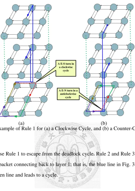
Fig. 3-5. Example of Rule 1 for (a) a Clockwise Cycle, and (b) a Counter-Clockwise Cycle. ... 25
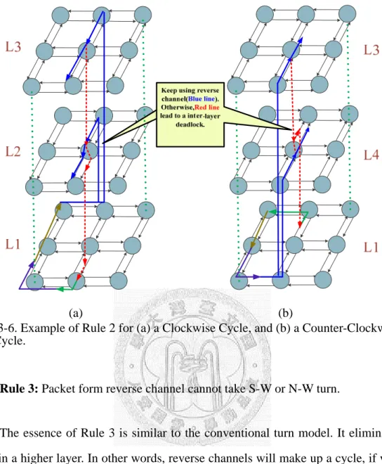
Fig. 3-6. Example of Rule 2 for (a) a Clockwise Cycle, and (b) a Counter-Clockwise Cycle. ... 26
Fig. 3-7. (a) Example of Rule 3, (b) Example of BI-routing, and (c) Traffic Condition Comparison. ... 27
Fig. 3-8. (a) Numbering of the Channels for the Bidirectional Routing, and (b) for each Input Channel and each Direction, the Output Channels Allowed by the Bidirectional Routing ... 29
vi
Fig. 3-9. Congested Situation in BiNoC ... 30 Fig. 3-10 TDM Concept ... 32 Fig. 3-11. Finite State Machine of Fluidity ... 33 Fig. 3-12. Stuck Problem in TDM-BiNoC ... 33 Fig. 4-1. A Node in Bidirectional Network-on-Chip ... 35 Fig. 4-2. Block Diagram of BiNoC Router ... 36 Fig. 4-3. InOut Buffer Block ... 37 Fig. 4-4. Algorithmic XY Routing Mechanism ... 38 Fig. 4-5. FSM for (a) High Priority FSM and (b) Low priority FSM ... 39 Fig. 4-6. Architecture of Matrix Arbiter ... 41 Fig. 4-7. An Example of 5x5 Multiplexer-Based Crossbar. ... 42 Fig. 4-8. Block Diagram of BI-Routing Router. ... 43 Fig. 4-9. Block Diagram of TDM-BiNoC Router. ... 44 Fig. 4-10. Router Interface in TDM-BiNoC ... 45 Fig. 5-1. Latency vs. Injection Rate Curve ... 48 Fig. 5-2. Throughput vs. Injection Rate Curve ... 48 Fig. 5-3. Latency versus Injection Rate under OE-Routing, WF-Routing,
XY-Routing, and BI-Routing ... 51 Fig. 5-4. throughput versus Injection Rate under OE-Routing, WF-Routing,
XY-Routing, and BI-Routing ... 52 Fig. 5-5. Flit Distribution Graph under (a) Odd-Even Routing Algorithm and (b)
Bidirectional Routing Algorithm. ... 53 Fig. 5-6. Histogram of Saturation Throughputs with XY-Routing, WF-Routing,
OE-Routing, and BI-Routing in Real Traffic Patterns ... 54 Fig. 5-7. Latency versus Injection Rate with Different Routing and Flow
Control Combinations ... 56 Fig. 5-8. Throughput versus Injection Rate with Different Routing and Flow
Control Combinations. ... 57 Fig. 5-9. Flits Distribution versus Latency for (a) BiNoC with OE-Routing, (b)
BiNoC with BI-Routing, and (c) TDM-BiNoC with OE-Routing ... 59 Fig. 5-10. Latency versus Injection Rate under Broadcast Traffic Pattern ... 60 Fig. 5-11. Area Distributions of (a) Bidirectional Routing and (b) TDM-BiNoC ... 62 Fig. A-1. Numbering of the Channels for the Bidirectional Routing. ... 67
Fig. A-3. A Part of an 8x8 Mesh NoC with Numbered Channels. ... 69
viii
LIST OF TABLES
Table 5-1. Performance Comparison between TDM-BiNoC and Original BiNoC .... 55 Table 5-2. Area Overhead of BI-Routing and TDM-BiNoC ... 61 Table 5-3. Power Overhead of BI-Routing and TDM-BiNoC ... 63
CHAPTER 1 INTRODUCTION
System-on-chip (SoC) uses numerous kinds of intellectual properties (IPs) and interconnections to make up a system in a single chip. As the technology progresses, the number and operating frequency of IPs are increasing. The bottleneck has transferred from IPs to interconnections. For example, with the 50nm technology, crossing a chip with a highly optimized interconnect takes between six to ten clock cycles and only one set of IPs can use the traditional bus-based interconnection to transact data such that the rest numerous IPs are waiting for the using right. Therefore, a new approach to designing the communication subsystem between IPs is proposed as network-on-chip (NoC). NoC has been proposed in the past years to meet the design productivity and signal integrity challenges of next-generation system designs [1][2][3].
1.1 Position of On-chip Interconnection in SoC
SoCs composed of several IPs and interconnections provide solutions in telecommunications, multimedia, and consumer electronics domains. Due to the time-to-market pressure, designers are used to reuse the pre-designed and pre-verified IPs which can be processors, controllers, or memory arrays to make up a well-performed SoC chip. However, as indicated in the International Technology Roadmap for Semiconductors (ITRS), IPs, using 50-nm where transistors are operating below one volt, can run at 10 GHZ. In regard to on-chip interconnection, where the finite propagation speed of electromagnetic waves, = (0.3 √ε⁄ ) mm per second in a homogeneous medium with relative permittivity ε, the chip die edge will be around 22mm in 50 nm technology. Thus, with an ideal ε, the delay for a signal to traverse the chip diagonally will take approximately one clock period. So the signal
2
propagated on a real-life interconnection is between six to ten clock cycles [4][5]. In conclusion, on-chip physical interconnection presents a limiting factor for performance and energy consumption.
1.2 Bus-Based Interconnection
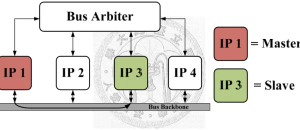
The conventional communication scheme in SoC is a bus-based interconnection, like the Advanced Microcontroller Bus Architecture (AMBA). It is usually composed of a shared-medium, an arbiter, a physical interface, multiplexers, and layered protocols. A bus-based structure is shown in Fig. 1-1.
Fig. 1-1. A Simple Representation of Bus-based Interconnection.
In a multi-core environment, we use parallel computing to speed up our system.
When the number of processing elements (PEs) is increasing, bus-based interconnection becomes very inefficient. The using right of the bus is owned by only one master PE and one slave PE with the rest PEs idle. The average communication bandwidth is very low when we have a certain large number of PEs. Besides, the more PEs are connected to the bus, the higher parasitic capacitance the bus has. Since the RC constant is higher, the bus-based interconnection will have a high latency and a high power consumption.
case-specific grouping of IP cores and design of different communication protocols to meet the requirements of each processing element. Low flexibility and reusability violate the rules in today’s SoC design.
1.3 Network-Based Interconnection: Network on Chip
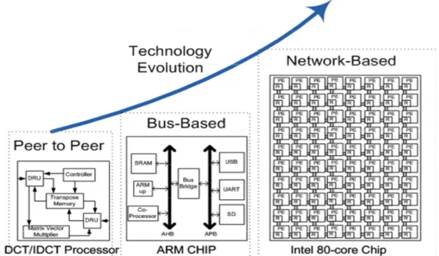
Network on Chip (NoC) is an innovative on-chip communication approach as shown in Fig. 1-2. Both Intel and Tilera Corporation have solved the multi-processor problem by using NoC architecture.
Fig. 1-2. An Example of Interconnection Evolution.
NoC is using the principles investigated for computer network to let IPs communicate with each other. Each IP has a network interface and a router so that data can be transformed into packet by the network interface and delivered by the router. Fig. 1-3 shows a simple configuration of NoC.
4
Fig. 1-3. A Simple Configuration of NoC.
Notice that NoC can let several sets of IPs communicate with each other. A network-based interconnection works like a computer network. Every IP which wants to send data can just transform the data into packets and deliver them through the on-chip network, such that IPs can operate again instead of waiting for the bus authority. In such a way, NoC helps to asynchronous design because IPs can operate on its own frequency. Asynchronous design is a popular research area, since it may speed up the system and reduce the clock tree. If we can reduce the clock tree, we will save the number of inverters used to decrease clock skew. Once the number of inverters is cut down, the whole chip has a lower power-consumption. Moreover, no matter how many IPs are contained in a chip, the parasitic capacitance keeps the same.
Since each IP is connected to only one router, and the number of connections in the router is fixed. As for flexibility and reusability, the on-chip router is feasible for all network size and all possible IPs. On account of this, we can find that NoC not only has higher communication speed but also lower power-consumption and higher reusability. These are what we need in VLSI design. Finally, we divide an NoC design into three basic categories: Topology, Routing, and Flow Control and give a simple introduction to each of these components on an NoC [6].
channels, and the topology of the network refers to the arrangement of these nodes and channels. Topology can be a line, ring, or tree depending on the application.
Deciding a topology is the first step to the design of an NoC. An appropriate topology will lead to a well-performed design.
We use a 2-Dimensional (2-D) mesh as our topology, because it is the most popular topology in NoC [7][8]. 2-D mesh means all the tiles are arranged like a square. An example of 2-D mesh is shown in Fig. 1-3. 2-D mesh has high scalability and its symmetry benefits to VLSI design.
Fig. 1-3. An NoC of 2-D Mesh.
1.3.2 Routing
Routing is to decide which path a packet is to deliver. In other words, given a source and a destination, routing directs a packet where to go. A bad routing algorithm will let numerous packets pass through the same path or choose a longer path. So routing algorithm determines the performance of NoC greatly.
We can divide routing algorithms in NoC design into two groups: deterministic routing algorithm [6] and adaptive routing algorithm [9][10]. The simplest routing algorithms are deterministic. They send every packet which has the same destination
6
and source to the same route. Therefore, we should realize that the same route will lead to the lack of path diversity, and it creates a large load imbalance in the network.
However, deterministic algorithms still have their merit depending on the application.
For example, if the topology of a router is irregular, to design a good adaptive algorithm is more difficult. Many early networks adopted deterministic routing because it was so simple and inexpensive to implement. As for adaptive routing, it uses information about the network state, typically queue occupancies, to select among alternative paths. There are minimal adaptive routing and non-minimal adaptive routing. Their difference is whether the packet can be delivered away from destination. Non-minimal routing has more choices on routing but often has a higher latency. However, non-minimal routing may encounte a livelock situation, where packets continue to move through the network, but never reach their destination. Most important of all, routing algorithms must be deadlock-free. A deadlock will cause the on-chip interconnection crashed. We will introduce more about routing algorithm in Chapter two.
1.3.3 Flow Control
How to allocate network resources, such as channel bandwidth, buffer capacity, and control state, is determined by flow control. There are buffered flow control and bufferless flow control, but considering the performance, we only use and introduce buffered flow control. The first kind of buffered flow control is store-and-forward flow control. It is the earliest buffered flow control. Its concept is very simple: when the entire packet is received in a router, the router forwards the packet. However, store-and-forward has a very high latency. Virtual cut-through flow control overcomes the latency problem of store-and-forward flow control by forwarding a packet as soon as the header is received and the resource of next hop is available. Virtual cut-through flow control saves much time from waiting for the whole packet to be received;
another better method is wormhole flow control. The difference of the virtual cut-through from the wormhole flow control is its dividing a packet into several flits,
1.4 Thesis Organization
The rest of this Thesis is organized as follows. In Chapter 2, we will first introduce the background about the architecture of BiNoC and several routing algorithms. Chapter 3 will describe a 3-dimensional model of BiNoC first. Then, A routing algorithm and a flow control mechanism based on the 3-dimensional model are presented. In Chapter 4, we will explain how we implement our router, and show the experimental simulation results in Chapter 5. Finally, Chapter 6 will draw a conclusion.
8
CHAPTER 2 BACKGROUND
In this chapter, we will present the architecture of bidirectional channel network on chip (BiNoC) in Section 2.1 [11][12]. In a conventional router, all channels is unidirectional, thus it may lead to the following scenario where one channel is busy or in congestion and another channel is idle because the direction of the idle channel is an input channel. BiNoC is proposed to overcome this problem by make all channels bidirectional. In Section 2.2, deadlock, deadlock-avoidance, and some deadlock-free routing algorithms will be introduced.
2.1 Bidirectional Channel in BiNoC
A bidirectional channel network-on-chip (BiNoC) architecture is proposed to enhance the performance of on-chip communication [11] [12]. The BiNoC allows each communication channel to be dynamically self-configured to transmit flits in either direction in order to better utilize on-chip hardware resources. For example, as shown in Fig. 2-1(a), every vertex represents a task with a value of its computation time, and every edge represents the computing dependence with a value of communication volume which is inverse of the bandwidth in a data channel. A mesh NoC with most optimized mapping is shown in Fig. 2-1(b). We can find that the NoC only use three channels with the other idle. A timing analysis in Fig. 2-2 indicates that conventional NoC needs 80 cycles to execute. However, if we make the same mapping solution on BiNoC which can dynamically change the direction of each channel between each pair of routers like the architecture in Fig. 2-3, the bandwidth utilization will be improved and the total execution time can be reduced to 55 cycles.
10
. (a) (b) (c)
Fig. 2-1. Example of (a) Task Graph Mapping to (b) a Conventional NoC, and (c) BiNoC [11].
Fig. 2-2. Detailed Execution Schedules of Typical NoC and BiNoC [11].
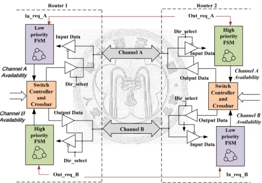
BiNoC reconfigures direction of channels by a request-based design as shown in Fig. 2-3, where the bidirectional channels are connected with an InOut Buffer to control the data conveyed from the bidirectional channel. Furthermore, we also need a finite state machine (FSM) to control the availability of each channel, or conflict will occur when both of the routers want to deliver packets. Once the availability signal is asserted, the Switch Controller can use the channel to deliver packets. The FSM will cooperate with another FSM in the downstream router such that only one direction is used to convey packet. For any direction of a router, a high priority channel is set up as a default direction. For example, in Fig. 2-3, channel A is a default link for router 2
In_req_A, will be sent to router 1, and router 1 will have no availability for channel A, which can prevent channel from changing direction frequently if both of the routers have packets to deliver. Moreover, it may lead to unfair issue, causing starvation.
Under this architecture, if both of the routers have packets to deliver, only one channel can be used for both of the routers. We will give a more detailed explanation on the router design in Chapter 4.
Fig. 2-3. Bidirectional Transmission Scheme.
2.2 Deadlock-Free Routing Algorithms
Routing algorithm influences the performance of NoC a lot. There are different routing algorithms for different applications. All have a common requirement that they must be deadlock-free. In this section, we will give a clear introduction of this issue.
12
2.2.1 Deadlock and Deadlock-Avoidance
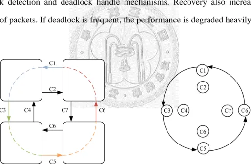
Deadlock is a crucial problem in NoC. Without an appropriate settling manner, the performance of interconnection network will be degraded very much, and even all the packets cannot be delivered to the destination. A theorem of deadlock avoidance proposed in [13] indicated that a connected and adaptive routing function R for an interconnection network I is deadlock-free if there is no cycle in its channel dependency graph (CDG). It is obvious by observing Fig. 2-4. The four packets at the four channels cannot make progress because they wait for each other cyclically.
Another way to deal with deadlock is deadlock recovery. We focus on deadlock avoidance in this work because deadlock recovery needs deadlock detection and deadlock handle mechanisms in addition. Overhead is thus increased, because of the deadlock detection and deadlock handle mechanisms. Recovery also increases the latency of packets. If deadlock is frequent, the performance is degraded heavily.
(a) (b)
Fig. 2-4. (a) A Deadlock Configuration and (b) Channel Dependency Graph.
2.2.2 XY Routing Algorithm
XY routing algorithm presented in [14] is a kind of deterministic routing algorithm.
With XY routing, a packet first traverses along the x dimension and then along the y dimension. XY routing is deadlock-free because no packet can traverse form y
a 2-D mesh NoC. However, for a given source and destination, XY routing always generates the same path such that XY routing has a poor load-balancing ability that leads to congestion problem. Fig. 2-5 gives an example.
Packet A
Packet B
Packet C
Fig. 2-5. An Example of XY Routing.
We can see that all of the three packets A, B, and C traverse along x dimension then along y dimension. Inevitably, some paths are congested with packets greatly like column 2 in Fig. 2-5.
2.2.3 Turn Model Based Routing Algorithm
Considering load balance, we prefer to use an adaptive routing algorithm that has more paths to choose for a packet delivery. There are two kinds of adaptive routing algorithms. One is minimal adaptive routing which routes a packet without using detour paths. Another is non-minimal adaptive routing which routes a packet with detour paths. However, non-minimal routing has to handle the livelock problem and its latency is higher, so we focus on minimal adaptive routing. Glass and Ni presented an elegant concept of turn model [15]. The basic idea of turn model is to prohibit the minimum number of turns that break all of the cycles in CDG such that
14
routing algorithms based on turn model can be deadlock-free. Three adaptive routing algorithms, namely west-first, north-last, and negative-first, are designed based on turn model. We show the four cases of prohibited turns of the three routing algorithms in Fig 2-6. Note that the solid lines indicate the allowed turns and the dash line indicate the prohibited turns. For example, Case two uses the turn model that prohibits S-W turn and N-W turn. According to this turn model, west-first routing delivers all the packets to west first if packets need to be delivered to west. Similar with the west-first routing, negative-first routing and north-last routing are designed according to the other turn models.
However, not all the turns can be used to prohibit deadlock. As indicated in Case four, a cycle will be generated if we use W-N turn in clockwise cycle and S-W in counterclockwise cycle. Turn model provides a simple way to design a deadlock-free adaptive routing, nevertheless, it is highly uneven in global view. At least half of the source-destination pairs are limited to having only one minimal path, while full adaptive is provided for the rest of the pairs.
Fig. 2-6. Four Cases of Turn Models.
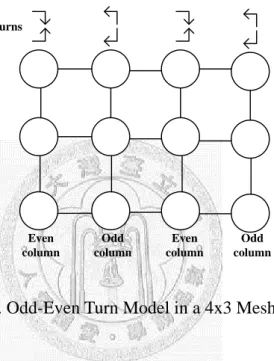
To solve the unfair problem in a turn model, an odd-even turn model was presented by Chiu in [10]. This odd-even turn model restricts certain turns based on the locations such that none of the turns are eliminated in an NoC. Chiu defined that a
packet is not allowed to take an E-N turn or an E-S turn at any nodes located in an even column, and any packet is not allowed to take an N-W turn or an S-W turn at any nodes located in an odd column. Fig. 2-7 shows the odd-even turn model in a 4x3 mesh.
Even column
Even column Odd
column
Odd column Restrict turns
Fig. 2-7. Odd-Even Turn Model in a 4x3 Mesh.
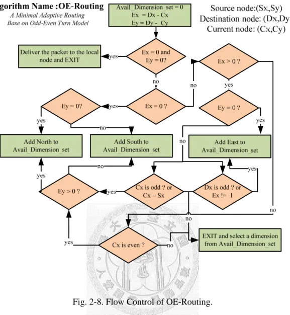
Although the odd-even still restricts some turns for a packet to use, these restricted turns are unobvious in global view. Therefore, the odd-even turn model has a higher path-diversity than the original turn model. Based on the odd-even turn model, we can design various deadlock-free adaptive routing. Fig. 2-8 shows an example that follows the odd-even turn model in an 8x8 mesh NoC. We call it OE-Routing.
16
Fig. 2-8. Flow Control of OE-Routing.
2.3 Another Implementation of Bidirectional Channel
Another work similar with BiNoC is bandwidth-adaptive NoC presented by Cho et al. [16]. The aim is same with BiNoC that using idle channel to increase bandwidth.
Nevertheless, a difference between BiNoC and bandwidth-adaptive NoC is that there are several bidirectional channels between two routers. They added a bandwidth allocator between two routers to decide the direction of channels. The bandwidth allocator uses a signal named pressure as input. The two routers send pressure to the bandwidth allocator and let this allocator to arbitrate the direction of channel. The block diagram is shown in Fig. 2-9.
Fig. 2-9. Connection Between two Network Nodes Through a Bidirectional Link [16].
With this architecture, bandwidth allocator can arbitrate more than two channels.
This allocator can dynamically decide how much bandwidth a router should have. An example is shown in Fig. 2-10.
Fig. 2-10. Adaptability of a Mesh Network with Bidirectional Links [16].
18
CHAPTER 3
MODELLING OF BIDIRECTIONAL-CHANNEL NOC
In this chapter, we present a three-dimensional model of BiNoC and two case studies that exploit the characteristics of bidirectional channels based on the three-dimensional model of BiNoC. One is a new routing algorithm for BiNoC called bidirectional routing (BI-Routing). BI-Routing uses the bidirectional channels to route packets and provides higher path-diversity. Another is a new mechanism called TDM-BiNoC which uses the time division multiplexing (TDM) concept to dynamically allocate the bandwidth of channels. Extensive simulation results shown in Chapter 5 indicate that these two works can improve the performance of a Mesh-based NoC.
3.1 Three-Dimensional Model of BiNoC
BiNoC can reduce packet latency and achieve higher bandwidth utilization by making channel bidirectional as shown in Fig. 3-1. Compared with the conventional NoC, both the two channels can switch their direction to generate four channel patterns.
Fig. 3-1. Variation of Channels in BiNoC.
20
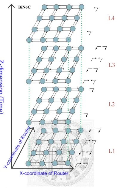
Since the original model of mesh NoC cannot show the behavior of BiNoC, we have to represent these four kinds of bidirectional channel patterns as a three-dimensional model in Fig. 3-2. The new Z-dimension is time related, which shows the channel diversity during time changed. Notice that not all the directions of channels in an NoC are changed in the different layers and we only care about the channel direction between two neighboring routers in a layer. In other words, we build our model in the view of one packet. Of course, we can just use any combination of these four patterns in a layer to represent the behavior of a BiNoC, but the combinations are too many and hard to represent or understand. The three-dimensional graph as shown in Fig. 3-2 is not a physical three-dimensional IC, but a conceptual model to represent the behavior of a BiNoC. We can use this model to express several researches related to BiNoC, like Quality of Service (QoS) [17] and fault tolerance [18]. In order to manage on-chip network resources adequately, traffic flow can be categorized in to guaranteed service (GS) and best effort (BE), and a QoS-BiNoC lets GS packets delivered to more layers in the model. Therefore GS packets can have higher path diversity than BE packets. As for fault-tolerance-BiNoC, our model indicates that bidirectional channels can have another layer to route when the channel of the original path fails. Moreover, as shown in Fig. 3-2, the odd even turn model in BiNoC can also be represented in our three-dimensional model. By using time division multiplexing concept, the odd even turn model in the three-dimensional model is complete. In other words, the odd even turn model in the L4 layer is complete when packets are delivered to the other layers like the L3 layer at another time. Besides, with this three-dimensional model, some good ideas pop out of our mind. We will show how to use this model to develop a routing algorithm and a time-division multiplexing mechanism for BiNoC.
Fig. 3-2. Three-Dimensional Model of BiNoC.
3.2 Bidirectional Routing Algorithm
The three-dimensional model of BiNoC mentioned in Section 3.1 indicates that BiNoC has higher path diversity than the original NoC. We use this path diversity to develop a BI-Routing algorithm for BiNoC in this section. After a brief explanation of motivation, we will introduce the detail of BI-Routing in Subsection 3.2.3.
3.2.1 Motivation of BI-Routing
In previous work, adaptive routing algorithms using turn model or odd-even turn model prohibiting some turns to prevent NoC from deadlock, hence, some paths are kept idle. The BI-Routing idea is shown in Fig. 3-3. On a conventional NoC, a
22
deadlock cycle formed by the paths of packet A, packet B, packet C, and packet D can be broken by using another layer of channel (in the Z-dimension). Therefore, we need not prohibit any turn and all paths can be included in the feasible routing set of BI-Routing.
Fig. 3-3. Cycles Breaking in BiNoC.
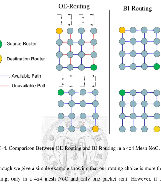
Figure 3-4 shows that the number of available paths of BI-Routing is much more than OE-routing. There are two cases in this example. In Case one, source is on the upper right corner and destination is on the lower left; in Case two, source is on the lower left and destination is on the upper right corner.
Fig. 3-4. Comparison Between OE-Routing and BI-Routing in a 4x4 Mesh NoC.
Though we give a simple example showing that our routing choice is more than OE-routing, only in a 4x4 mesh NoC and only one packet sent. However, if the topology size is larger, the more advantage we can take.
3.2.2 Bidirectional Routing
Bidirectional routing (BI-Routing) is a minimal adaptive routing algorithm. As mentioned in Subsection 3.1.2, BI-Routing is deadlock-free without prohibiting any path. We develop the BI-Routing based on Theorem 1 brought up by Duato [19].
Theorem 1: A connected and adaptive routing function R for an interconnection network I is deadlock-free, if there are no cycles in its channel dependency graph [19].
24
A channel dependency graph D for a given interconnection network I and routing function R is a directed graph, D = G(C, E). The vertices of D are the channels of I. The arcs of D are the pairs of channels ( , ) such that there is a direct dependency from to . The meaning of connected routing function is that for any packet, the connected routing function can find a path to deliver the packet to the destination.
Therefore, from Theorem 1, if we can break the cycle in a channel dependency graph, the routing algorithm is deadlock-free. Hence, three rules are brought up for our BI-Routing algorithm.
Rule 1: Packets use reverse channel at the E-S turn and the E-N turn.
As mentioned in Subsection 3.1.2, we escape from deadlock in an BiNoC by using another layer to route, as shown in Fig. 3-3. Here, we choose E-S turn and E-N turn as a breaking position in clockwise and counter-clockwise cycles. An example is shown in Fig. 3-5, where the red lines mean a path which will lead to deadlock, and our concept is represented by blue lines which escape from the deadlock cycle by using a reverse channel in BiNoC. There are two conditions on what the direction of another channel is. Thus, we use two blue lines in the two layers to represent all these two network paths. In other words, packets use L2 or L3 to route when taking an E-S turn as shown in Fig. 3-5(a), and packets use L4 and L3 to route when taking and an E-N turn as shown in Fig. 3-5(b). Although Fig. 3-5 just shows one cycle in clockwise and counter-clockwise, any other cycle does not exist in the network because of Rule 1. However, it is oblivious that Rule 1 is not sufficient to remove deadlock. A cycle may happen after we take Rule 1, so we still need another rule.
A E-N turn in a anticlockwise
cycle A E-S turn in
a clockwise cycle
L1 L1
L2 L4
(a) (b)
Fig. 3-5. Example of Rule 1 for (a) a Clockwise Cycle, and (b) a Counter-Clockwise Cycle.
We use Rule 1 to escape from the deadlock cycle. Rule 2 and Rule 3 are needed to avoid a packet connecting back to layer 1; that is, the blue line in Fig. 3-5 connects back to green line and leads to a cycle.
Rule 2. Packets from south (north) reverse channel and delivered to north (south) must use reverse channel.
An inter-layer deadlock will appear without Rule 2. Rule 2 indicates that packets should keep using a reserve channel in south or north such that an inter-layer deadlock can be removed. In the view of three-dimensional model, packets keep using L2 (L3) to route when delivered from north in the L2 (L3) layer as shown in Fig.
3-6(a), and packets keep using L4 (L3) to route when delivered form south in the L4 (L3) layer as shown in Fig. 3-6(b). An example is shown in Fig. 3-6, where blue lines represent paths obeying Rule 2, and red dotted lines represent paths violating Rule 2.
26
(a) (b)
Fig. 3-6. Example of Rule 2 for (a) a Clockwise Cycle, and (b) a Counter-Clockwise Cycle.
Rule 3: Packet form reverse channel cannot take S-W or N-W turn.
The essence of Rule 3 is similar to the conventional turn model. It eliminates a turn in a higher layer. In other words, reverse channels will make up a cycle, if we do not have rule to regulate packets. In the view of three-dimensional model, packets cannot take S-W turn and N-W turn when packets are not in the L1 layer. For a more clear understanding, Fig. 3-7(a) shows an example, where the red dotted lines represent prohibiting turns in a higher layer. From Theorem 1, BI-Routing is deadlock-free because these three rules keep the channel dependency acyclic. A more detailed example is shown in Fig. 3-7(b) and a traffic condition comparison is shown in Fig. 3-7(c).
(a)
(b) (c)
Fig. 3-7. (a)Example of Rule 3, (b) Example of BI-routing, and (c) Traffic Condition Comparison.
28
In Fig. 3-7(b), P4 is transferred to an upper layer by Rule 1, and breaks a cycle which may be constructed from P6, P7, and P8. Another bigger cycle may be constructed from P6, P7, P9, and P3. However, Rule 1 holds it back at P3. Rule 2 plays an important role in preventing BI-Routing from an inter-layer deadlock. Notice that only reverse-south channel and reverse-north channel are in the scope of Rule 2, and packets can be routed to east freely. P2 and P1 have explained these cases. P2 in a middle layer connects back to a bottom layer, as shown in Fig. 3-7(b). Nevertheless, Rule 1 stops P1 from forming a deadlock cycle. At last, an inter-layer cycle does not exist in the top layer because of Rule 3.
Although we still need three rules to acquire our BI-Routing algorithm, we provide a fully adaptive routing algorithm. Fully adaptive routing algorithm can spread traffic load to the whole network instead of keeping some parts of network in heavy congestion. Fig. 3-7(c) shows the comparison of OE-routing and BI-Routing. In OE-routing, three packets have no other choices but to route on the same path, leading a congestion node and two minor congestion nodes. Contrarily, in our BI-Routing, those three packets have much more choices and can be delivered to at most two dimensions, thus can choose paths that increase the balance of BiNoC.
To avoid limitation by these three rules, we design a selection function that prefers paths, other than the E-S turn and E-N turn. After all the other paths are in use, the selection function then considers Rule 1 and so on. Notice that this selection function is only applied to south and north input buffers. All the other is still in a round-robin way.
3.2.3 Deadlock-Free Proof for Bidirectional Routing
Dally and Seitz showed that a routing algorithm is deadlock-free if the channels in the communication network can be numbered, and the routing algorithm routes packets along channels with strictly increasing numbers [20]. Actually, if packets are delivered with a strictly increasing order, there are no cycles in the channel
(a)
m-x-1, y+1 m+x, y+1
m+x, n-y m-x-1, n-y
x, y
m-x-1, 0
m-x-1, 0 m-x, 0
m-x, 0
From East
m+x, n-y m-x-1, n-y
x, y
m-x, 0
m-x, 0
m-x-1, n-y-1
m+x+1, 0
m+x+1, 0
m+x+1, 0
m+x+1, 0 m-x, 0
m-x, 0
m-x-1, y+1 m+x, y+1
m-x-1, y
x, y
m+x, n-y
x, y
m+x+1, 0
m+x+1, 0 m+x, n-y-1
m+x+1, 0
m+x+1, 0 m+x, y+1
m+x, n-y
x, y
m+x, 0
m+x, 0
m+x+1, 0
m+x+1, 0 m+x, y+1
x, y
m+x, y From West
Rule 1
From South (Normal Channel)
From South (Reverse Channel) Rule 2&Rule 3 From North (Reverse Channel)
Rule 2 &Rule 3 From North (Normal Channel)
(b)
Fig. 3-8. (a) Numbering of the Channels for the Bidirectional Routing, and (b) For each Input Channel and each Direction, the Output Channels Allowed by the Bidirectional Routing.
30
We show all the cases in Fig. 3-8(b). For each channel and direction, the output channels allowed by the bidirectional routing are strictly increasing. Therefore, according to the proof by Dally and Seitz, the bidirectional routing algorithm is deadlock-free (A detailed illustration is described in Appendix A). Our proof is similar with the work by Glass and Ni [21]. However, our bidirectional routing is based on wormhole BiNoC instead of virtual channel BiNoC.
3.3 Time Division Multiplexing on BiNoC
In this section, we will present a new mechanism derived from the time division multiplexing concept of nowadays communication system. This mechanism can balance packets between routers, unlike BI-Routing, which increases the balance of traffic load by supplying more routing paths in the whole BiNoC chip.
3.3.1 Motivation
In a BiNoC, routers reconfigure the direction of channels only when the downstream router does not use the channel. However, if the traffic load of one router is much higher than another downstream router and both routers have to use the same channel to deliver, the BiNoC cannot accommodate this situation. An example is shown in Fig. 3-9. Both of Node 2 and Node 5 have packets to deliver, so BiNoC cannot switch the direction of its channel. Thus, Node 5 is congested and also influences the neighbor node.
The bandwidth-adaptive NoC mentioned in Section 2.3 can accommodate this situation. Unlike the request-based design of BiNoC, bandwidth-adaptive NoC is a pressure-based design. The bandwidth allocator receives the pressure signal from two neighboring nodes such that allocator has the information of congestion and controls the direction of multiple channels to release congestion. We use the concept of time division multiplexing on BiNoC to solve this problem.
Time division multiplexing (TDM) is an application of time division concept in which many signals can be seemingly transferred simultaneously as on the sub-channels in one physical channel, but indeed take turns on the channel. On the
Fig. 3-9. Congested Situation in BiNoC.
Recalling Fig. 3-2(b), the Z-coordinate of the three-dimensional model of BiNoC represents time, and direction of channel changes according to time variation. So we can associate BiNoC with TDM. Sub-channels in TDM are the bidirectional channels in BiNoC and the access authority of a physical channel is determined by the routers.
We can dynamically allocate packets in the different layers of a three-dimensional model of BiNoC according to the traffic load. We call such a BiNoC with a TDM mechanism as TDM-BiNoC.
3.3.2 TDM Mechanism in BiNoC
We will present a clearer concept of our TDM-BiNoC mechanism in this section.
Fig. 3-10 shows the concept of TDM-BiNoC mechanism. Assume that there are two routers, Routers A and B, and A is doubly congested than B. In this situation, our TDM-BiNoC mechanism can allocate a time-variant channel direction according to the traffic load. Therefore, if Router A is doubly congested than Router B, Router A owns two time units to deliver packets and Router B has one time unit. Namely,
32
TDM-BiNoC can dynamically allocate different time units for different traffic loads.
Hence, by the time division multiplexing concept, our TDM-BiNoC can change its channel ratio flexibly instead of 1 or 0.5 in the original BiNoC.
Fig. 3-10. TDM Concept.
Therefore, the TDM-BiNoC can be viewed as virtually adding multiple channels in Fig. 3-10, in the same way as a bandwidth-adaptive NoC. Moreover, we get up to the bandwidth-adaptive NoC without adding wiring area between routers. The wiring area between routers is critical in an NoC design. There is no doubt that the example in Fig. 3-9 is an extreme example, but this situation increases latency greatly and indeed exists. Our TDM-BiNoC can benefit from the case where the traffic load is asymmetric, like Fig. 3-9.
3.3.3 Fluidity Mechanism in TDM-BiNoC
Conventional congestion control scheme is using buffer fill-level information which indicates what level a buffer is filled. Fluidity concept was presented by Tsai et al. in [22]. It is intuitive to conclude that fluidity can reflect congestion degree in a buffer without explanation. Beside the buffer fill-level, fluidity concept not only points out the capacity of a buffer but also indicates how fluent packets in the buffer are. In other words, a buffer containing many packets can still has a high frequency to pass packets and fluidity concept can represent such case.
The color depth of these states is different. The more deep the color, the less fluid the buffer is. In the Inactive state, the buffer is empty such that any incoming flit of a packet can go through the buffer quickly. Once the buffer is not empty, the current state is transferred into Fluid0. Fluid0 will be transferred into a more un-fluent state, Fluid1, if no flit passes out during a pre-defined period. The transition of Fluid1 and Nonfluid is similar with Fluid0. A current state is transferred according to the behavior of a buffer such that this FSM can reflect the fluidity of the buffer. All of the above three states are transferred to Inactive when all flits pass out.
Fig. 3-11. Finite State Machine of Fluidity.
Our TDM-BiNoC uses fluidity as index information to allocate a time unit to each router. The router with lower fluidity will acquire more time units to deliver.
However, as shown in Fig. 3-12, the packets from a low-fluidity router may suffer blockage and becomes un-fluent again. Then, we allocate more time units for those packets in vain. Therefore, we modify the arbitration in the crossbar to help our TDM-BiNoC. The arbiter in a crossbar needs to give the router with a lower fluidity a higher priority. By doing this, we can make packets flow smoothly in the BiNoC.
34
Fig. 3-12. Stuck Problem in TDM-BiNoC
The aim of BI-Routing and TDM-BiNoC is to increase load balance in a communication network, but they are achieving such goal in different aspects.
BI-Routing owns more routing paths to select, thus increasing balance in the whole chip. As for TDM-BiNoC, it considers the router-to-router load balance.
Unfortunately, it is hard to combine BI-Routing with TDM-BiNoC, because both of BI-Routing and TDM-BiNoC use the same bidirectional characteristic of a channel.
They cannot cooperate with each other, and bidirectional channel cannot afford over-exploitation. The detailed simulation results will be given in Chapter 5.
CHAPTER 4
ROUTER ARCHITECTURE
An NoC is composed of several basic nodes. Fig. 4-1 shows a basic node in BiNoC, where data generated by an IP are transformed into packets and sent to the Network Interface. Then, on-chip communication is done by the On-Chip Router. We will present our router architecture in this chapter. The original BiNoC router [11]
composed of several basic components will be presented in Section 4.1. Two versions of this router, modified with BI-Routing and TDM-BiNoC, will be presented in Section 4.2. In Chapter 5, we will show the simulation results of BiNoC with 64 routers.
Fig. 4-1. A Node in Bidirectional Network-on-Chip.
36
4.1 BiNoC Router Architecture
The block diagram of a BiNoC router is shown in Fig. 4-2. Packets conveyed in the data path are controlled by control blocks. Datapath is composed of an InOut Buffer, an Input Buffer Unit, and a Crossbar. Control blocks contain a Routing Computation Unit, a Switch Allocator, a Request Manager, and a Channel Controller.
Besides, we use registers in our design to prevent the router from glitch and to pipeline our router design. Pipeline can reduce the critical timing of a router design, and improve throughput. We use a pipeline of three stages in our design: routing computation, switch arbitration, and flit transmission. We do not use virtual channel in our router to save area, lower power consumption, and reduce latency.
Fig. 4-2. Block Diagram of BiNoC Router.
anarchy that the output data may influence the input blocks in the neighboring router.
An InOut Buffer as shown in Fig. 4-3 will solve such problem. The InOut Buffer is composed of two tri-state buffers. Either an output enable or an input enable can be asserted, which controls the connection of a bidirectional channel to the router.
InOut Buffer
Input Data
Output Data
Dir_select
Fig. 4-3. InOut Buffer Block.
Buffers can be constructed by centralized buffers, independent buffers at the input port, or independent buffers at the output port. We use buffers constructed by independent buffers at each input port in this work, each of which is a First-In-First-Out buffer composed of shift registers.
4.1.2 Routing Computation Unit
We can implement a routing computation unit by two kinds of mechanisms:
table-based routing and algorithm-based routing. For table-based routing, packets get decisions by a look-up table at the source node or at each node along the route to compute their destination depending on the application. The major advantage of table-based routing is its generality, where source-table routing only computes the destination of a packet once, and node-table routing is more appropriate for adaptive routing. A routing table can support any routing relation and suitable for any topology by simply reprogramming the contents of the table.
38
Algorithmic routing implements the routing algorithm as a combinational logic circuit dedicated to the routing strategy and topology. Fig. 4-4 shows the algorithmic routing mechanism implementing an XY routing algorithm. This architecture uses six comparators and one direction selector. For every header flit, the related locations of the current router and the destination router will be reset by comparing the destination router ID and the current router ID, and then the Direction Selector will pick an optimal direction. Owing to the lower area overhead needed in an NoC, we use an algorithmic routing mechanism instead of a table-based routing mechanism in our Routing Computation Unit.
Fig. 4-4. Algorithmic XY Routing Mechanism.
4.1.3 Request Manager and Channel Controller
As mentioned in Section 2-1, BiNoC is a request-based design. If a router requests to use a channel with low priority, it must make sure that the downstream router needs not to use it. All requests are sent by the Request Manager. The concept of Request Manager is very simple. That is, it will send a request to the low-priority channel if the router has more than one packet to deliver. Otherwise, the request manager will just send a request to the high priority channel. Our Channel Controller is implemented with a high-priority and a low-priority channel-control FSMs as shown in Fig. 4-5. Both of the FSMs have three states: wait, free, and idle
˙ Idle state: The channel cannot deliver data, and it is being used to receive data.
˙ Wait state: An intermediate state from the idle state to the free state.
(a)
wait free
idle
count = 4 &&
input_req = 0 output_req = 1
count++
output_req = channel_req
output_req = 0 count = 0 input_req = 1
count < 4 &&
input_req = 0
input_req = 0
input_req = 1
channel_req = 0 ||
input_req = 1 channel_req = 1 &&
input_req = 0
(b)
Fig. 4-5. FSM for (a) High Priority FSM and (b) Low priority FSM.
40
A bidirectional channel is controlled by a high-priority FSM and a low-priority FSM. The two FSMs will coordinate with each other such that only one direction is used. In other words, there exists not the case of two free states. If one FSM is at a free state, another FSM is at an idle or a wait state according to the transferring condition. The high-priority FSM uses a free state as the default state. If the neighbor router wants to deliver a packet, input_req will be asserted and if there is no channel request in this router, FSM will be transformed into an idle state. Then, if there is a channel request in this router, FSM will be transformed into a wait state right away. After two clock cycles of waiting for the neighbor FSM to complete its operation, the FSM in this router is transformed into a free state. As to the low-priority FSM, the transferring condition is stricter. The wait state in the low-priority FSM may turn back to an idle state when any input request occurs.
4.1.4 Switch Allocator and Crossbar
After a routing direction is determined, packets contend for the channel. Therefore, we need an arbiter to allocate the channel bandwidth to the requesters. We use ten arbiters in our Switch Allocator block. All requests to an output channel will be arbitrated with an arbiter, and these requests may be masked by the channel available signal. These arbiters are implemented by a matrix-arbiter as shown in Fig. 4-6. A matrix arbiter implements a least-recently served priority scheme by updating a triangular array of state bits ω for < . The state bits in row © and column j show that request © takes priority over request j. We only update the upper triangular portion of the matrix, because the value at the lower triangular portion is just the inverse of the upper one. After a request is granted, the bit in that row is cleared, and the bit in that column is set to give that request the lowest priority since it was the most recently served. Notice that not all the state bit values are legal for a request. For example, if ω = ω = 1 and ω = 0 and requests 0, 1, and 2 are all asserted, the request will disable each other. Matrix arbiter is easy, inexpensive to implement, and provides strong fairness [6].
Fig. 4-6. Architecture of Matrix Arbiter.
We need a Crossbar to connect every input buffer and every output channel such that flits can be switched. In this work, we use multiplexers to implement our Crossbar as shown in Fig. 4-7. The crossbar consists of ten 5-to-1 multiplexers, where each multiplexer corresponds to an output port. The selecting signal comes from the Switch Allocator. Though the input of a BiNoC crossbar is twice than that in an NoC, the area overhead of a crossbar is acceptable. However, for n inputs, an n2 area is needed to contain the n2 crosspoints, and another n2 area is needed to hold n multiplexers. This is another reason that we do not use virtual channel, because it will make the cost of crossbar too high to have more input buffers in each direction of the channel. Our router must be small enough to fit in an NoC.
42
Fig. 4-7. An Example of 5x5 Multiplexer-Based Crossbar.
4.2 Implementations of BI-Routing and TDM-BiNoC Routers
We need to modify the Routing Computation Unit, Switch Allocator, and Request Manager to implement a BI-Routing router as shown in Fig. 4-8. We replace the algorithmic-based OE-routing in the Routing Computation Unit with our BI-Routing algorithm. Thus, we modify the selecting function as follows. We prefer directions that do not consider to take Rule 1. After all the channels of the selected direction are occupied, we can then use the direction that observes Rule 1. The Routing Computation Unit outputs a routing direction and a signal called reverse_channel. This signal is asserted when the result of the Routing Computation Unit is claimed to use a reverse channel, and transmitted to Switch Allocator, such that the packets can be delivered via this reverse channel, and the signal be transmitted to the downstream router to acquire the reverse channel.
We will present the implementation of our TDM-BiNoC router in the following paragraph. Compared with this TDM-BiNoC router, the overhead of BI-Routing router is lower. More discussion and results will be presented in Chapter 5.
Fig. 4-8. Block Diagram of BI-Routing Router.
We carry out our TDM-BiNoC router based on the architecture as shown in Fig.
4-8. The Input Buffer Unit is equipped with a fluidity FSM to monitor the buffer as mentioned in Section 3.2.3. Hence, FSM can release the fluidity information to a directional fluidity generator (DF-Generator). This DF-Generator uses both the fluidity information from Input Buffer Unit and the result from the Routing Computation Unit as inputs so that it can compute the information on directional fluidity. Here the directional fluidity is defined as the total fluidity of packets which would be delivered to each direction of the channel. The directional fluidity is passed on to every neighboring router. Therefore, given such directional fluidity information, a router has its local congestion information and neighboring router’s congestion information for each direction of the channel. A Request Controller is added to implement our TDM-concept. The Request Controller arbitrates the accessing time
44
slot to control the direction of a channel based on the directional fluidity information.
The Request Controller will cooperate with another Request Controller in the neighboring router. Thus, the channel can switch direction standing on the congestion consideration. We show the block diagram of the TDM-BiNoC router in Fig. 4-9 and its router interface in Fig. 4-10.
Fig. 4-9. Block Diagram of TDM-BiNoC Router.
Fig. 4-10. Router Interface in TDM-BiNoC
In the Router Interface of the TDM-BiNoC as shown in Fig. 4-10, a Directional Fluidity signal is added to control the communication between each pair of neighboring routers. Obviously, the wiring area is increased heavily because this cost exists at every direction of a channel in a router. However, we can control the width of directional fluidity in the design to gain the best performance. We will show the detailed area overhead in Chapter 5.
46
CHAPTER 5 EXPERIMENTAL RESULTS
In order to compare the performance and hardware cost between the several routing algorithms and our bidirectional routing algorithm, we implemented a cycle-accurate simulation environment in HDL language, Verilog [23]. We simulated routing algorithms in an 8x8 mesh NoC composed of 64 routers without consideration of the effect of processing elements.
In the following sections, we first introduce the performance evaluation, synthetic traffic patterns and real traffic patterns in Section 5.1. Simulation results with several routing algorithms are given in Section 5.2, and simulation results with TDM-BiNOC in Section 5.3. Implementation overhead is presented in Section 5.4.
5.1 Background of Network Simulation
We introduce the background of network simulation in this section. First, performance evaluation is presented in Subsection 5.1.1. Then, traffic patterns are presented in Subsection 5.1.2.
5.1.1 Performance of Interconnection Networks.
Performance of an interconnection network can be described by its latency vs.
injection rate curve as shown in Fig. 5.1. At low injection rate, latency is close to a zero-load latency, . Zero-load latency means that the injected packet never contends for network resources with other packets. As the injection rate increasing, latency goes to infinity at the saturation throughput, λ . Saturation throughput can be slightly less than the bound of Θ if a flow control method is applied to the network, but it is limited by the topology bound of 2 ⁄ , and no routing algorithm R can exceed this limitation.
48
Fig. 5-1. Latency vs. Injection Rate Curve [6].
Although the above latency graph reveals the performance of a network at its extremes, it does not show the average behavior of the network. The throughput of a network as shown in Fig. 5-2 is linear at low injection rate until the injection rate reaches a saturation point. Using this information, we can calculate the average behavior of a network.
Fig. 5-2. Throughput vs. Injection Rate Curve [6].
5.1.2 Synthetic Traffic Patterns and Real Traffic Patterns
Our simulation environment comprised an 8x8 mesh array that can handle both synthetic traffic patterns [24] and real traffic patterns [25] as the simulation inputs.
Three types of synthetic traffic patterns were used to run simulations, including
randomized destination with a probability based on the injection rate. In the transpose traffic, a node at a source with coordinate (i, j) will sent a packet to a destination with coordinate (j,i). In the hotspot traffic, 20% of the packets change their destination to some selected hotspots while the remaining 80% of the traffic keep uniform. In this work, we chose (3, 3), (3, 2), (3, 1), (3, 0) as hotspots.
In addition to the synthetic traffics, we used Embedded System Synthesis Benchmarks Suite (E3S) benchmarks to demonstrate the performance variations in real traffics. Three applications of E3S, auto-indust-cords, consumer-cords, and telecom-cords, are mapped to a 5x5, a 4x4, and a 6x6 mesh networks respectively. In this work, we adopted a common Simulated Annealing algorithm to map task graphs given in E3S to our NoC.
5.2 Simulation Results of Routing Algorithms
We simulated XY-Routing, west first routing algorithm (WF-Routing), odd even routing (OE-Routing), and our bidirectional routing (BI-Routing) algorithms and show the results in this section. The packets in our experiments were composed of 16 flits with one header flit and one tail flit. The capacity of the buffer in each of the 5 directions of channels was 8 flits. Considering the practicability of NoC, we used wormhole switching to manage the buffer instead of virtual channel, because the area overhead of virtual channel is pretty much. We simulated our network by injecting loads, from 20 flits per clock cycle to 500 flits per clock, at every node. For each injection rate, the simulation time was 25000 clock cycles. The results of latency in three synthetic traffic patterns are shown in Fig. 5-3, and the results of throughput are shown in Fig. 5-4.