Modern Compiler Implementation in C

(1)

(2)

Modern Compiler Implementation in C

(3)

(4)

Modern Compiler Implementation in C

ANDREW W. APPEL

Princeton University

with MAIA GINSBURG

(5)

CAMBRIDGE UNIVERSITY PRESS

The Edinburgh Building, Cambridge CB2 2RU, UK 40 West 20th Street, New York NY 10011–4211, USA 477 Williamstown Road, Port Melbourne, VIC 3207, Australia Ruiz de Alarcón 13, 28014 Madrid, Spain

Dock House, The Waterfront, Cape Town 8001, South Africa http://www.cambridge.org

This book is in copyright. Subject to statutory exception and to the provisions of relevant collective licensing agreements, no reproduction of any part may take place without

the written permission of Cambridge University Press.

First published 1998

Revised and expanded edition of Modern Compiler Implementation in C: Basic Techniques Reprinted with corrections, 1999

First paperback edition 2004

Typeset in Times, Courier, and Optima

A catalogue record for this book is available from the British Library Library of Congress Cataloguing-in-Publication data

Appel, Andrew W., 1960–

Modern compiler implementation in C / Andrew W. Appel with Maia Ginsburg. – Rev.

and expanded ed.

x, 544 p. : ill. ; 24 cm.

Includes bibliographical references (p. 528–536) and index.

ISBN 0 521 58390 X (hardback)

1. C (Computer program language) 2. Compilers (Computer programs) I. Ginsburg, Maia. II. Title.

QA76.73.C15A63 1998

005.4´53—dc21 97-031089 CIP ISBN 0 521 58390 X hardback

ISBN 0 521 60765 5 paperback

Information on this title:www.cambridge.org/9780521583909

(6)

Preface

Over the past decade, there have been several shifts in the way compilers are built. New kinds of programming languages are being used: object-oriented languages with dynamic methods, functional languages with nested scope and first-class function closures; and many of these languages require garbage collection. New machines have large register sets and a high penalty for memory access, and can often run much faster with compiler assistance in scheduling instructions and managing instructions and data for cache locality.

This book is intended as a textbook for a one- or two-semester course in compilers. Students will see the theory behind different components of a compiler, the programming techniques used to put the theory into practice, and the interfaces used to modularize the compiler. To make the interfaces and programming examples clear and concrete, I have written them in the C programming language. Other editions of this book are available that use the Java and ML languages.

Implementation project. The “student project compiler” that I have outlined is reasonably simple, but is organized to demonstrate some important techniques that are now in common use: abstract syntax trees to avoid tangling syntax and semantics, separation of instruction selection from register allocation, copy propagation to give flexibility to earlier phases of the compiler, and containment of target-machine dependencies. Unlike many “student compilers” found in textbooks, this one has a simple but sophisticated back end, allowing good register allocation to be done after instruction selection.

Each chapter in Part Ihas a programming exercise corresponding to one module of a compiler. Software useful for the exercises can be found at

http://www.cs.princeton.edu/˜appel/modern/c

(11)

Exercises. Each chapter has pencil-and-paper exercises; those marked with a star are more challenging, two-star problems are difficult but solvable, and the occasional three-star exercises are not known to have a solution.

Course sequence. The figure shows how the chapters depend on each other.

1. Introduction 2. Lexical

Analysis 3. Parsing 4. Abstract

Syntax 5.Semantic Analysis

6.Activation Records

9.Instruction

Selection 12.Putting it

All Together

10.Liveness Analysis

13.Garbage

Collection 14.Object-Oriented Languages 17.Dataflow

Analysis 18.Loop

Optimizations

20.Pipelining, Scheduling

21.Memory Hierarchies 19.

Static Single- Assignment Form 11.Register

Allocation

15.Functional

Languages 16.Polymorphic Types 7.Translation to

Intermediate Code 8.Basic Blocks and Traces

QuarterQuarter SemesterSemester

• A one-semester course could cover all ofPart I(Chapters 1–12), with students implementing the project compiler (perhaps working in groups); in addition, lectures could cover selected topics fromPart II.

• An advanced or graduate course could cover Part II, as well as additional topics from the current literature. Many of thePart IIchapters can stand inde- pendently fromPart I, so that an advanced course could be taught to students who have used a different book for their first course.

• In a two-quarter sequence, the first quarter could coverChapters 1–8, and the second quarter could coverChapters 9–12and some chapters fromPart II.

Acknowledgments. Many people have provided constructive criticism or helped me in other ways on this book. I would like to thank Leonor Abraido- Fandino, Scott Ananian, Stephen Bailey, Max Hailperin, David Hanson, Jef- frey Hsu, David MacQueen, Torben Mogensen, Doug Morgan, Robert Netzer, Elma Lee Noah, Mikael Petterson, Todd Proebsting, Anne Rogers, Barbara Ryder, Amr Sabry, Mooly Sagiv, Zhong Shao, Mary Lou Soffa, Andrew Tol- mach, Kwangkeun Yi, and Kenneth Zadeck.

(12)

PART ONE

Fundamentals of

Compilation

(13)

(14)

1

Introduction

A compiler was originally a program that “compiled”

subroutines [a link-loader]. When in 1954 the combina- tion “algebraic compiler” came into use, or rather into misuse, the meaning of the term had already shifted into the present one.

Bauer and Eickel [1975]

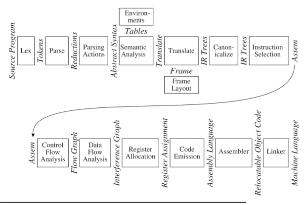
This book describes techniques, data structures, and algorithms for translating programming languages into executable code. A modern compiler is often organized into many phases, each operating on a different abstract “language.”

The chapters of this book follow the organization of a compiler, each covering a successive phase.

To illustrate the issues in compiling real programming languages, I show how to compile Tiger, a simple but nontrivial language of the Algol family, with nested scope and heap-allocated records. Programming exercises in each chapter call for the implementation of the corresponding phase; a student who implements all the phases described in Part I of the book will have a working compiler. Tiger is easily modified to be functional or object-oriented (or both), and exercises inPart IIshow how to do this. Other chapters inPart IIcover advanced techniques in program optimization. Appendix A describes the Tiger language.

The interfaces between modules of the compiler are almost as important as the algorithms inside the modules. To describe the interfaces concretely, it is useful to write them down in a real programming language. This book uses the C programming language.

(15)

Source Program Tokens Reductions Abstract Syntax Translate Tables

Frame

IR Trees IR Trees Assem

Assem Flow Graph Interference Graph Register Assignment Assembly Language Relocatable Object Code Machine Language

Parsing Actions Parse

Lex Semantic

Analysis Translate Canon- icalize

Frame Layout Environ-

ments

Instruction Selection

Control Flow Analysis

Data Flow Analysis

Register Allocation

Code

Emission Assembler Linker

FIGURE 1.1. Phases of a compiler, and interfaces between them.

1.1 MODULES AND INTERFACES

Any large software system is much easier to understand and implement if the designer takes care with the fundamental abstractions and interfaces.Fig- ure 1.1shows the phases in a typical compiler. Each phase is implemented as one or more software modules.

Breaking the compiler into this many pieces allows for reuse of the components. For example, to change the target-machine for which the compiler produces machine language, it suffices to replace just the Frame Layout and In- struction Selection modules. To change the source language being compiled, only the modules up through Translate need to be changed. The compiler can be attached to a language-oriented syntax editor at the Abstract Syntax interface.

The learning experience of coming to the right abstraction by several itera- tions of think–implement–redesign is one that should not be missed. However, the student trying to finish a compiler project in one semester does not have

(16)

1.2. TOOLS AND SOFTWARE

this luxury. Therefore, I present in this book the outline of a project where the abstractions and interfaces are carefully thought out, and are as elegant and general as I am able to make them.

Some of the interfaces, such as Abstract Syntax, IR Trees, and Assem, take the form of data structures: for example, the Parsing Actions phase builds an Abstract Syntaxdata structure and passes it to the Semantic Analysis phase.

Other interfaces are abstract data types; the Translate interface is a set of functions that the Semantic Analysis phase can call, and the Tokens interface takes the form of a function that the Parser calls to get the next token of the input program.

DESCRIPTION OF THE PHASES

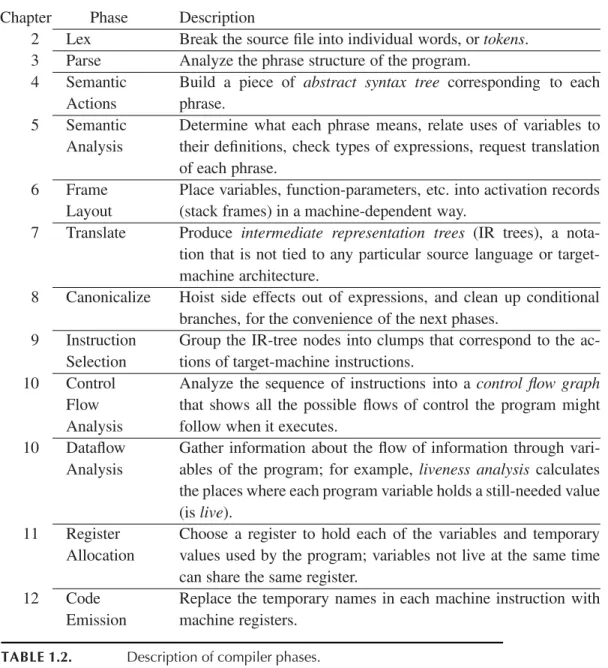
Each chapter ofPart Iof this book describes one compiler phase, as shown in Table 1.2

This modularization is typical of many real compilers. But some compilers combine Parse, Semantic Analysis, Translate, and Canonicalize into one phase; others put Instruction Selection much later than I have done, and combine it with Code Emission. Simple compilers omit the Control Flow Analy- sis, Data Flow Analysis, and Register Allocation phases.

I have designed the compiler in this book to be as simple as possible, but no simpler. In particular, in those places where corners are cut to simplify the implementation, the structure of the compiler allows for the addition of more optimization or fancier semantics without violence to the existing interfaces.

1.2 TOOLS AND SOFTWARE

Two of the most useful abstractions used in modern compilers are context- free grammars, for parsing, and regular expressions, for lexical analysis. To make best use of these abstractions it is helpful to have special tools, such as Yacc (which converts a grammar into a parsing program) and Lex (which converts a declarative specification into a lexical analysis program).

The programming projects in this book can be compiled using any ANSI- standard C compiler, along with Lex (or the more modern Flex) and Yacc (or the more modern Bison). Some of these tools are freely available on the Internet; for information see the World Wide Web page

http://www.cs.princeton.edu/˜appel/modern/c

(17)

Chapter Phase Description

2 Lex Break the source file into individual words, or tokens.

3 Parse Analyze the phrase structure of the program.

4 Semantic Actions

Build a piece of abstract syntax tree corresponding to each phrase.

5 Semantic Analysis

Determine what each phrase means, relate uses of variables to their definitions, check types of expressions, request translation of each phrase.

6 Frame

Layout

Place variables, function-parameters, etc. into activation records (stack frames) in a machine-dependent way.

7 Translate Produce intermediate representation trees (IR trees), a nota- tion that is not tied to any particular source language or target- machine architecture.

8 Canonicalize Hoist side effects out of expressions, and clean up conditional branches, for the convenience of the next phases.

9 Instruction Selection

Group the IR-tree nodes into clumps that correspond to the actions of target-machine instructions.

10 Control Flow Analysis

Analyze the sequence of instructions into a control flow graph that shows all the possible flows of control the program might follow when it executes.

10 Dataflow Analysis

Gather information about the flow of information through vari- ables of the program; for example, liveness analysis calculates the places where each program variable holds a still-needed value (is live).

11 Register Allocation

Choose a register to hold each of the variables and temporary values used by the program; variables not live at the same time can share the same register.

12 Code

Emission

Replace the temporary names in each machine instruction with machine registers.

TABLE 1.2. Description of compiler phases.

Source code for some modules of the Tiger compiler, skeleton source code and support code for some of the programming exercises, example Tiger programs, and other useful files are also available from the same Web address.

The programming exercises in this book refer to this directory as $TIGER/

when referring to specific subdirectories and files contained therein.

(18)

1.3. DATA STRUCTURES FOR TREE LANGUAGES

Stm → Stm ; Stm (CompoundStm) Stm →id :=Exp (AssignStm) Stm →print(ExpList ) (PrintStm)

Exp →id (IdExp)

Exp →num (NumExp)

Exp → Exp Binop Exp (OpExp) Exp → ( Stm , Exp ) (EseqExp)

ExpList → Exp , ExpList (PairExpList) ExpList → Exp (LastExpList)

Binop → + (Plus)

Binop → − (Minus)

Binop → × (Times)

Binop → / (Div)

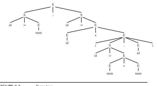
GRAMMAR 1.3. A straight-line programming language.

1.3 DATA STRUCTURES FOR TREE LANGUAGES

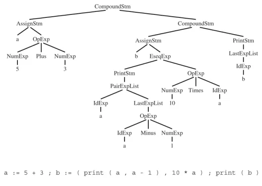
Many of the important data structures used in a compiler are intermediate representations of the program being compiled. Often these representations take the form of trees, with several node types, each of which has different attributes. Such trees can occur at many of the phase-interfaces shown in Figure 1.1.

Tree representations can be described with grammars, just like programming languages. To introduce the concepts, I will show a simple programming language with statements and expressions, but no loops or if-statements (this is called a language of straight-line programs).

The syntax for this language is given inGrammar 1.3.

The informal semantics of the language is as follows. Each Stm is a state- ment, each Exp is an expression. s₁;s₂executes statement s₁, then statement s₂. i:=e evaluates the expression e, then “stores” the result in variable i.

print(e₁,e₂, . . . ,e_n) displays the values of all the expressions, evaluated left to right, separated by spaces, terminated by a newline.

An identifier expression, such as i, yields the current contents of the vari- able i. A number evaluates to the named integer. An operator expression e₁ op e₂ evaluates e₁, then e₂, then applies the given binary operator. And an expression sequence (s, e) behaves like the C-language “comma” opera- tor, evaluating the statement s for side effects before evaluating (and returning the result of) the expression e.

(19)

CompoundStm.

AssignStm

a OpExp

NumExp 5

Plus NumExp 3

CompoundStm

AssignStm b EseqExp

PrintStm PairExpList IdExp

a

LastExpList OpExp IdExp

a

Minus NumExp 1

OpExp NumExp

10

Times IdExp a

PrintStm LastExpList

IdExp b

a := 5 + 3 ; b := ( print ( a , a - 1 ) , 10 * a ) ; print ( b )

FIGURE 1.4. Tree representation of a straight-line program.

For example, executing this program

a := 5+3; b := (print(a, a-1), 10*a); print(b)

prints

8 7 80

How should this program be represented inside a compiler? One represen- tation is source code, the characters that the programmer writes. But that is not so easy to manipulate. More convenient is a tree data structure, with one node for each statement (Stm) and expression (Exp).Figure 1.4shows a tree representation of the program; the nodes are labeled by the production labels ofGrammar 1.3, and each node has as many children as the corresponding grammar production has right-hand-side symbols.

We can translate the grammar directly into data structure definitions, as shown inProgram 1.5.Each grammar symbol corresponds to a typedef in the data structures:

(20)

Grammar typedef

Stm A stm

Exp A exp

ExpList A expList

id string

num int

For each grammar rule, there is one constructor that belongs to theunion for its left-hand-side symbol. The constructor names are indicated on the right-hand side ofGrammar 1.3.

Each grammar rule has right-hand-side components that must be represented in the data structures. The CompoundStm has two Stm’s on the right- hand side; the AssignStm has an identifier and an expression; and so on. Each grammar symbol’s struct contains a unionto carry these values, and a kindfield to indicate which variant of the union is valid.

For each variant (CompoundStm, AssignStm, etc.) we make a constructor functiontomallocand initialize the data structure. InProgram 1.5only the prototypes of these functions are given; the definition of A_CompoundStm would look like this:

A_stm A_CompoundStm(A_stm stm1, A_stm stm2) { A_stm s = checked_malloc(sizeof(*s));

s->kind = A_compoundStm;

s->u.compound.stm1=stm1; s->u.compound.stm2=stm2;

return s;

}

For Binop we do something simpler. Although we could make a Binop struct – with union variants for Plus, Minus, Times, Div – this is overkill because none of the variants would carry any data. Instead we make anenum typeA_binop.

Programming style. We will follow several conventions for representing tree data structures in C:

1. Trees are described by a grammar.

2. A tree is described by one or more typedefs, corresponding to a symbol in the grammar.

3. Each typedef defines a pointer to a corresponding struct. The struct name, which ends in an underscore, is never used anywhere except in the declaration of the typedef and the definition of the struct itself.

4. Each struct contains a kind field, which is an enum showing different variants, one for each grammar rule; and a u field, which is a union.

(21)

typedef char *string;

typedef struct A_stm_ *A_stm;

typedef struct A_exp_ *A_exp;

typedef struct A_expList_ *A_expList;

typedef enum {A_plus,A_minus,A_times,A_div} A_binop;

struct A_stm_ {enum {A_compoundStm, A_assignStm, A_printStm} kind;

union {struct {A_stm stm1, stm2;} compound;

struct {string id; A_exp exp;} assign;

struct {A_expList exps;} print;

} u;

};

A_stm A_CompoundStm(A_stm stm1, A_stm stm2);

A_stm A_AssignStm(string id, A_exp exp);

A_stm A_PrintStm(A_expList exps);

struct A_exp_ {enum {A_idExp, A_numExp, A_opExp, A_eseqExp} kind;

union {string id;

int num;

struct {A_exp left; A_binop oper; A_exp right;} op;

struct {A_stm stm; A_exp exp;} eseq;

} u;

};

A_exp A_IdExp(string id);

A_exp A_NumExp(int num);

A_exp A_OpExp(A_exp left, A_binop oper, A_exp right);

A_exp A_EseqExp(A_stm stm, A_exp exp);

struct A_expList_ {enum {A_pairExpList, A_lastExpList} kind;

union {struct {A_exp head; A_expList tail;} pair;

A_exp last;

} u;

};

PROGRAM 1.5. Representation of straight-line programs.

5. If there is more than one nontrivial (value-carrying) symbol in the right-hand side of a rule (example: the rule CompoundStm), the union will have a component that is itself a struct comprising these values (example: the compound element of the A_stm_ union).

6. If there is only one nontrivial symbol in the right-hand side of a rule, the union will have a component that is the value (example: the num field of the A_exp union).

7. Every class will have a constructor function that initializes all the fields. The malloc function shall never be called directly, except in these constructor functions.

(22)

8. Each module (header file) shall have a prefix unique to that module (example, A_ inProgram 1.5).

9. Typedef names (after the prefix) shall start with lowercase letters; constructor functions (after the prefix) with uppercase; enumeration atoms (after the prefix) with lowercase; and union variants (which have no prefix) with lowercase.

Modularity principles for C programs. A compiler can be a big program;

careful attention to modules and interfaces prevents chaos. We will use these principles in writing a compiler in C:

1. Each phase or module of the compiler belongs in its own “.c” file, which will have a corresponding “.h” file.

2. Each module shall have a prefix unique to that module. All global names (structure and union fields are not global names) exported by the module shall start with the prefix. Then the human reader of a file will not have to look outside that file to determine where a name comes from.

3. All functions shall have prototypes, and the C compiler shall be told to warn about uses of functions without prototypes.

4. We will #include "util.h" in each file:

/* util.h */

#include <assert.h>

typedef char *string;

string String(char *);

typedef char bool;

#define TRUE 1

#define FALSE 0

void *checked_malloc(int);

The inclusion of assert.h encourages the liberal use of assertions by the C programmer.

5. The string type means a heap-allocated string that will not be modified af- ter its initial creation. The String function builds a heap-allocated string from a C-style character pointer (just like the standard C library function strdup). Functions that take strings as arguments assume that the contents will never change.

6. C’s malloc function returns NULL if there is no memory left. The Tiger compiler will not have sophisticated memory management to deal with this problem. Instead, it will never call malloc directly, but call only our own function, checked_malloc, which guarantees never to return NULL:

(23)

void *checked_malloc(int len) { void *p = malloc(len);

assert(p);

return p;

}

7. We will never call free. Of course, a production-quality compiler must free its unused data in order to avoid wasting memory. The best way to do this is to use an automatic garbage collector, as described inChapter 13(see partic- ularly conservative collection on page 296). Without a garbage collector, the programmer must carefully free(p) when the structure p is about to become inaccessible – not too late, or the pointer p will be lost, but not too soon, or else still-useful data may be freed (and then overwritten). In order to be able to concentrate more on compiling techniques than on memory deallocation techniques, we can simply neglect to do any freeing.

P R O G R A M STRAIGHT-LINE PROGRAM INTERPRETER

Implement a simple program analyzer and interpreter for the straight-line programming language. This exercise serves as an introduction to environ- ments(symbol tables mapping variable-names to information about the vari- ables); to abstract syntax (data structures representing the phrase structure of programs); to recursion over tree data structures, useful in many parts of a compiler; and to a functional style of programming without assignment state- ments.

It also serves as a “warm-up” exercise in C programming. Programmers experienced in other languages but new to C should be able to do this exercise, but will need supplementary material (such as textbooks) on C.

Programs to be interpreted are already parsed into abstract syntax, as described by the data types inProgram 1.5.

However, we do not wish to worry about parsing the language, so we write this program by applying data constructors:

A_stm prog =

A_CompoundStm(A_AssignStm("a",

A_OpExp(A_NumExp(5), A_plus, A_NumExp(3))), A_CompoundStm(A_AssignStm("b",

A_EseqExp(A_PrintStm(A_PairExpList(A_IdExp("a"),

A_LastExpList(A_OpExp(A_IdExp("a"), A_minus, A_NumExp(1))))), A_OpExp(A_NumExp(10), A_times, A_IdExp("a")))), A_PrintStm(A_LastExpList(A_IdExp("b")))));

(24)

PROGRAMMING EXERCISE

Files with the data type declarations for the trees, and this sample program, are available in the directory$TIGER/chap1.

Writing interpreters without side effects (that is, assignment statements that update variables and data structures) is a good introduction to denota- tional semantics and attribute grammars, which are methods for describing what programming languages do. It’s often a useful technique in writing compilers, too; compilers are also in the business of saying what programming languages do.

Therefore, in implementing these programs, never assign a new value to any variable or structure-field except when it is initialized. For local variables, use the initializing form of declaration (for example, int i=j+3;) and for each kind of struct, make a “constructor” function that allocates it and initializes all the fields, similar to theA_CompoundStmexample on page 9.

1. Write a function int maxargs(A_stm) that tells the maximum number of arguments of any print statement within any subexpression of a given statement. For example, maxargs(prog) is 2.

2. Write a function void interp(A_stm) that “interprets” a program in this language. To write in a “functional programming” style – in which you never use an assignment statement – initialize each local variable as you declare it.

For part 1, remember that print statements can contain expressions that contain other print statements.

For part 2, make two mutually recursive functions interpStm and interpExp. Represent a “table,” mapping identifiers to the integer values assigned to them, as a list ofid×intpairs.

typedef struct table *Table_;

struct table {string id; int value; Table_ tail};

Table_ Table(string id, int value, struct table *tail) { Table_ t = malloc(sizeof(*t));

t->id=id; t->value=value; t->tail=tail;

return t;

}

The empty table is represented asNULL. TheninterpStmis declared as

Table_ interpStm(A_stm s, Table_ t)

taking a table t₁ as argument and producing the new table t₂ that’s just like t₁ except that some identifiers map to different integers as a result of the statement.

(25)

For example, the table t₁that maps a to 3 and maps c to 4, which we write {a $→3, c $→ 4} in mathematical notation, could be represented as the linked

list _{a 3} _{c 4} .

Now, let the table t₂be just like t₁, except that it maps c to 7 instead of 4.

Mathematically, we could write, t₂=update(t₁,c,7)

where the update function returns a new table {a $→ 3, c $→ 7}.

On the computer, we could implement t₂by putting a new cell at the head of the linked list: _{c 7} _{a 3} _{c 4} as long as we assume that the first occurrence of c in the list takes precedence over any later occur- rence.

Therefore, theupdatefunction is easy to implement; and the correspond- inglookupfunction

int lookup(Table_ t, string key)

just searches down the linked list.

Interpreting expressions is more complicated than interpreting statements, because expressions return integer values and have side effects. We wish to simulate the straight-line programming language’s assignment statements without doing any side effects in the interpreter itself. (Theprintstatements will be accomplished by interpreter side effects, however.) The solution is to declareinterpExpas

struct IntAndTable {int i; Table_ t;};

struct IntAndTable interpExp(A_exp e, Table_ t) · · ·

The result of interpreting an expression e₁with table t₁ is an integer value i and a new table t₂. When interpreting an expression with two subexpressions (such as anOpExp), the table t₂resulting from the first subexpression can be used in processing the second subexpression.

F U R T H E R R E A D I N G

Hanson [1997] describes principles for writing modular software in C.

(26)

EXERCISES

E X E R C I S E S

1.1 This simple program implementspersistent functional binary search trees, so that if tree2=insert(x,tree1), then tree1 is still available for lookups even while tree2 can be used.

typedef struct tree *T_tree;

struct tree {T_tree left; String key; T_tree right;};

T_tree Tree(T_tree l, String k, T_tree r) { T_tree t = checked_malloc(sizeof(*t));

t->left=l; t->key=k; t->right=r;

return t;

}

T_tree insert(String key, T_tree t) { if (t==NULL) return Tree(NULL, key, NULL) else if (strcmp(key,t->key) < 0)

return Tree(insert(key,t->left),t->key,t->right);

else if (strcmp(key,t->key) > 0)

return Tree(t->left,t->key,insert(key,t->right));

else return Tree(t->left,key,t->right);

}

a. Implement amemberfunction that returnsTRUEif the item is found, else FALSE.

b. Extend the program to include not just membership, but the mapping of keys to bindings:

T_tree insert(string key, void *binding, T_tree t);

void * lookup(string key, T_tree t);

c. These trees are not balanced; demonstrate the behavior on the following two sequences of insertions:

(a) t s p i p f b s t (b) a b c d e f g h i

*d. Research balanced search trees in Sedgewick [1997] and recommend a balanced-tree data structure for functional symbol tables. Hint: To preserve a functional style, the algorithm should be one that rebalances on insertion but not on lookup, so a data structure such assplay treesis not appropriate.

(27)

2

Lexical Analysis

lex-i-cal: of or relating to words or the vocabulary of a language as distinguished from its grammar and construction

Webster’s Dictionary

To translate a program from one language into another, a compiler must first pull it apart and understand its structure and meaning, then put it together in a different way. The front end of the compiler performs analysis; the back end does synthesis.

The analysis is usually broken up into

Lexical analysis: breaking the input into individual words or “tokens”;

Syntax analysis: parsing the phrase structure of the program; and Semantic analysis: calculating the program’s meaning.

The lexical analyzer takes a stream of characters and produces a stream of names, keywords, and punctuation marks; it discards white space and comments between the tokens. It would unduly complicate the parser to have to account for possible white space and comments at every possible point; this is the main reason for separating lexical analysis from parsing.

Lexical analysis is not very complicated, but we will attack it with high- powered formalisms and tools, because similar formalisms will be useful in the study of parsing and similar tools have many applications in areas other than compilation.

(28)

2.1. LEXICAL TOKENS

2.1 LEXICAL TOKENS

A lexical token is a sequence of characters that can be treated as a unit in the grammar of a programming language. A programming language classifies lexical tokens into a finite set of token types. For example, some of the token types of a typical programming language are:

Type Examples

ID foo n14 last

NUM 73 0 00 515 082

REAL 66.1 .5 10. 1e67 5.5e-10

IF if

COMMA ,

NOTEQ !=

LPAREN (

RPAREN )

Punctuation tokens such asIF,VOID,RETURNconstructed from alphabetic characters are called reserved words and, in most languages, cannot be used as identifiers.

Examples of nontokens are

comment /* try again */

preprocessor directive #include<stdio.h>

preprocessor directive #define NUMS 5 , 6

macro NUMS

blanks, tabs, and newlines

In languages weak enough to require a macro preprocessor, the preprocessor operates on the source character stream, producing another character stream that is then fed to the lexical analyzer. It is also possible to integrate macro processing with lexical analysis.

Given a program such as

float match0(char *s) /* find a zero */

{if (!strncmp(s, "0.0", 3)) return 0.;

}

the lexical analyzer will return the stream

FLOAT ID(match0) LPAREN CHAR STAR ID(s) RPAREN

LBRACE IF LPAREN BANG ID(strncmp) LPAREN ID(s)

(29)

COMMA STRING(0.0) COMMA NUM(3) RPAREN RPAREN

RETURN REAL(0.0) SEMI RBRACE EOF

where the token-type of each token is reported; some of the tokens, such as identifiers and literals, have semantic values attached to them, giving auxil- iary information in addition to the token type.

How should the lexical rules of a programming language be described? In what language should a lexical analyzer be written?

We can describe the lexical tokens of a language in English; here is a description of identifiers in C or Java:

An identifier is a sequence of letters and digits; the first character must be a letter. The underscore _ counts as a letter. Upper- and lowercase letters are different. If the input stream has been parsed into tokens up to a given character, the next token is taken to include the longest string of characters that could possibly constitute a token. Blanks, tabs, newlines, and comments are ignored except as they serve to separate tokens. Some white space is required to separate otherwise adjacent identifiers, keywords, and constants.

And any reasonable programming language serves to implement an ad hoc lexer. But we will specify lexical tokens using the formal language of regular expressions, implement lexers using deterministic finite automata, and use mathematics to connect the two. This will lead to simpler and more readable lexical analyzers.

2.2 REGULAR EXPRESSIONS

Let us say that a language is a set of strings; a string is a finite sequence of symbols. The symbols themselves are taken from a finite alphabet.

The Pascal language is the set of all strings that constitute legal Pascal programs; the language of primes is the set of all decimal-digit strings that represent prime numbers; and the language of C reserved words is the set of all alphabetic strings that cannot be used as identifiers in the C programming language. The first two of these languages are infinite sets; the last is a finite set. In all of these cases, the alphabet is the ASCII character set.

When we speak of languages in this way, we will not assign any meaning to the strings; we will just be attempting to classify each string as in the language or not.

To specify some of these (possibly infinite) languages with finite descrip-

(30)

2.2. REGULAR EXPRESSIONS

tions, we will use the notation of regular expressions. Each regular expression stands for a set of strings.

Symbol: For each symbol a in the alphabet of the language, the regular expres- sion a denotes the language containing just the string a.

Alternation: Given two regular expressions M and N, the alternation operator written as a vertical bar | makes a new regular expression M | N. A string is in the language of M | N if it is in the language of M or in the language of N. Thus, the language of a | b contains the two strings a and b.

Concatenation: Given two regular expressions M and N, the concatenation operator · makes a new regular expression M · N. A string is in the language of M · N if it is the concatenation of any two strings α and β such that α is in the language of M and β is in the language of N. Thus, the regular expression (a | b) · a defines the language containing the two strings aa and ba.

Epsilon: The regular expression ϵ represents a language whose only string is the empty string. Thus, (a · b) | ϵ represents the language {"","ab"}.

Repetition: Given a regular expression M, its Kleene closure is M^∗. A string is in M^∗if it is the concatenation of zero or more strings, all of which are in M. Thus, ((a | b) · a)^∗represents the infinite set { "" , "aa", "ba", "aaaa",

"baaa", "aaba", "baba", "aaaaaa", . . . }.

Using symbols, alternation, concatenation, epsilon, and Kleene closure we can specify the set of ASCII characters corresponding to the lexical tokens of a programming language. First, consider some examples:

(0 | 1)^∗·0 Binary numbers that are multiples of two.

b^∗(abb^∗)^∗(a|ϵ) Strings ofa’s andb’s with no consecutivea’s.

(a|b)^∗aa(a|b)^∗ Strings ofa’s andb’s containing consecutivea’s.

In writing regular expressions, we will sometimes omit the concatenation symbol or the epsilon, and we will assume that Kleene closure “binds tighter”

than concatenation, and concatenation binds tighter than alternation; so that ab | c means (a · b) | c, and (a |) means (a | ϵ).

Let us introduce some more abbreviations: [abcd] means (a | b | c | d), [b-g] means [bcdefg], [b-gM-Qkr] means [bcdefgMNOPQkr], M?

means (M | ϵ), and M⁺means (M·M^∗). These extensions are convenient, but none extend the descriptive power of regular expressions: Any set of strings that can be described with these abbreviations could also be described by just the basic set of operators. All the operators are summarized inFigure 2.1.

Using this language, we can specify the lexical tokens of a programming language (Figure 2.2). For each token, we supply a fragment of C code that reports which token type has been recognized.

(31)

a An ordinary character stands for itself.

ϵ The empty string.

Another way to write the empty string.

M | N Alternation, choosing from M or N.

M · N Concatenation, an M followed by an N.

M N Another way to write concatenation.

M^∗ Repetition (zero or more times).

M⁺ Repetition, one or more times.

M? Optional, zero or one occurrence of M.

[a − zA − Z] Character set alternation.

. A period stands for any single character except newline.

"a.+*" Quotation, a string in quotes stands for itself literally.

FIGURE 2.1. Regular expression notation.

if {return IF;}

[a-z][a-z0-9]* {return ID;}

[0-9]+ {return NUM;}

([0-9]+"."[0-9]*)|([0-9]*"."[0-9]+) {return REAL;}

("--"[a-z]*"\n")|(" "|"\n"|"\t")+ { /* do nothing */ }

. {error();}

FIGURE 2.2. Regular expressions for some tokens.

The fifth line of the description recognizes comments or white space, but does not report back to the parser. Instead, the white space is discarded and the lexer resumed. The comments for this lexer begin with two dashes, contain only alphabetic characters, and end with newline.

Finally, a lexical specification should be complete, always matching some initial substring of the input; we can always achieve this by having a rule that matches any single character (and in this case, prints an “illegal character”

error message and continues).

These rules are a bit ambiguous. For example, doesif8match as a single identifier or as the two tokensifand8? Does the stringif 89begin with an identifier or a reserved word? There are two important disambiguation rules used by Lex and other similar lexical-analyzer generators:

Longest match: The longest initial substring of the input that can match any regular expression is taken as the next token.

Rule priority: For a particular longest initial substring, the first regular expres-

(32)

2.3. FINITE AUTOMATA

i

1 2 3

f

2 1

a-z a-z

0-9 1 2

0-9 0-9

IF ID NUM

0-9

0-9 0-9

5

1 3

4 0-9

.

2

.

0-9

\n

5 1

blank, etc.

2 a-z

3 4

blank, etc.

- -

any but \n

1 2

REAL white space error

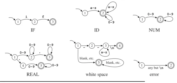
FIGURE 2.3. Finite automata for lexical tokens. The states are indicated by circles; final states are indicated by double circles. The start state has an arrow coming in from nowhere. An edge labeled with several characters is shorthand for many parallel edges.

sion that can match determines its token type. This means that the order of writing down the regular-expression rules has significance.

Thus,if8matches as an identifier by the longest-match rule, andifmatches as a reserved word by rule-priority.

2.3 FINITE AUTOMATA

Regular expressions are convenient for specifying lexical tokens, but we need a formalism that can be implemented as a computer program. For this we can use finite automata (N.B. the singular of automata is automaton). A finite automaton has a finite set of states; edges lead from one state to another, and each edge is labeled with a symbol. One state is the start state, and certain of the states are distinguished as final states.

Figure 2.3shows some finite automata. We number the states just for convenience in discussion. The start state is numbered 1 in each case. An edge labeled with several characters is shorthand for many parallel edges; so in theIDmachine there are really 26 edges each leading from state 1 to 2, each labeled by a different letter.

(33)

\n 1

a-z 2

-

3 4

13 12

9 11

6

7 8

10 5

i

0-9

.

0-9

f 0-9 0-9

- 0-9, a-z

a-hj-z

other blank,

etc.

blank, etc.

ID IF ID REAL

NUM REAL

error

white space white space

error error

a-z0-9 a-e, g-z, 0-9

.

FIGURE 2.4. Combined finite automaton.

In a deterministic finite automaton (DFA), no two edges leaving from the same state are labeled with the same symbol. A DFA accepts or rejects a string as follows. Starting in the start state, for each character in the input string the automaton follows exactly one edge to get to the next state. The edge must be labeled with the input character. After making n transitions for an n-character string, if the automaton is in a final state, then it accepts the string. If it is not in a final state, or if at some point there was no appropriately labeled edge to follow, it rejects. The language recognized by an automaton is the set of strings that it accepts.

For example, it is clear that any string in the language recognized by automaton IDmust begin with a letter. Any single letter leads to state 2, which is final; so a single-letter string is accepted. From state 2, any letter or digit leads back to state 2, so a letter followed by any number of letters and digits is also accepted.

In fact, the machines shown inFigure 2.3accept the same languages as the regular expressions ofFigure 2.2.

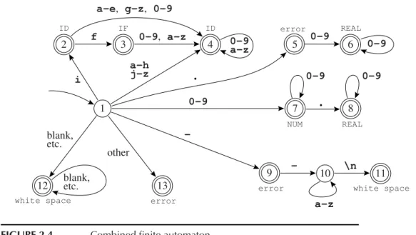
These are six separate automata; how can they be combined into a single machine that can serve as a lexical analyzer? We will study formal ways of doing this in the next section, but here we will just do it ad hoc:Figure 2.4 shows such a machine. Each final state must be labeled with the token-type

(34)

2.3. FINITE AUTOMATA

that it accepts. State 2 in this machine has aspects of state 2 of theIFmachine and state 2 of theIDmachine; since the latter is final, then the combined state must be final. State 3 is like state 3 of theIF machine and state 2 of theID

machine; because these are both final we use rule priority to disambiguate – we label state 3 with IF because we want this token to be recognized as a reserved word, not an identifier.

We can encode this machine as a transition matrix: a two-dimensional array (a vector of vectors), subscripted by state number and input character.

There will be a “dead” state (state 0) that loops to itself on all characters; we use this to encode the absence of an edge.

int edges[][256]={ /* · · ·0 1 2· · ·-· · ·e f g h i j· · · */

/* state 0 */ {0,0,· · ·0,0,0· · ·0· · ·0,0,0,0,0,0· · ·}, /* state 1 */ {0,0,· · ·7,7,7· · ·9· · ·4,4,4,4,2,4· · ·}, /* state 2 */ {0,0,· · ·4,4,4· · ·0· · ·4,3,4,4,4,4· · ·}, /* state 3 */ {0,0,· · ·4,4,4· · ·0· · ·4,4,4,4,4,4· · ·}, /* state 4 */ {0,0,· · ·4,4,4· · ·0· · ·4,4,4,4,4,4· · ·}, /* state 5 */ {0,0,· · ·6,6,6· · ·0· · ·0,0,0,0,0,0· · ·}, /* state 6 */ {0,0,· · ·6,6,6· · ·0· · ·0,0,0,0,0,0· · ·}, /* state 7 */ {0,0,· · ·7,7,7· · ·0· · ·0,0,0,0,0,0· · ·}, /* state 8 */ {0,0,· · ·8,8,8· · ·0· · ·0,0,0,0,0,0· · ·},

et cetera }

There must also be a “finality” array, mapping state numbers to actions – final state 2 maps to actionID, and so on.

RECOGNIZING THE LONGEST MATCH

It is easy to see how to use this table to recognize whether to accept or reject a string, but the job of a lexical analyzer is to find the longest match, the longest initial substring of the input that is a valid token. While interpreting transitions, the lexer must keep track of the longest match seen so far, and the position of that match.

Keeping track of the longest match just means remembering the last time the automaton was in a final state with two variables,Last-Final(the state number of the most recent final state encountered) andInput-Position- at-Last-Final. Every time a final state is entered, the lexer updates these variables; when a dead state (a nonfinal state with no output transitions) is reached, the variables tell what token was matched, and where it ended.

Figure 2.5shows the operation of a lexical analyzer that recognizes longest matches; note that the current input position may be far beyond the most recent position at which the recognizer was in a final state.

(35)

Last Current Current Accept

Final State Input Action

0 1 ⊤⊥if --not-a-com|

2 2 |i⊤⊥f --not-a-com

3 3 |if⊤⊥ --not-a-com

3 0 ^|if⊤⊥--not-a-com returnIF

0 1 if|⊤⊥ --not-a-com

12 12 if|⊤⊥--not-a-com

12 0 if|⊤-⊥-not-a-com found white space; resume

0 1 if |⊤⊥--not-a-com

9 9 if |-⊤⊥-not-a-com

9 10 if |-⊤-⊥not-a-com

9 10 if |-⊤-n⊥ot-a-com

9 10 if |-⊤-no⊥t-a-com

9 10 if |-⊤-not⊥-a-com

9 0 if |-⊤-not-⊥a-com error, illegal token ‘-’; resume

0 1 if -|⊤⊥-not-a-com

9 9 if -|-⊤⊥not-a-com

9 0 if -|-⊤n⊥ot-a-com error, illegal token ‘-’; resume FIGURE 2.5. The automaton of Figure 2.4 recognizes several tokens. The

symbol | indicates the input position at each successive call to the lexical analyzer, the symbol ⊥ indicates the current position of the automaton, and ⊤ indicates the most recent position in which the recognizer was in a final state.

2.4 NONDETERMINISTIC FINITE AUTOMATA

A nondeterministic finite automaton (NFA) is one that has a choice of edges – labeled with the same symbol – to follow out of a state. Or it may have special edges labeled with ϵ (the Greek letter epsilon), that can be followed without eating any symbol from the input.

Here is an example of an NFA:

a a a a

a

(36)

2.4. NONDETERMINISTIC FINITE AUTOMATA

In the start state, on input charactera, the automaton can move either right or left. If left is chosen, then strings ofa’s whose length is a multiple of three will be accepted. If right is chosen, then even-length strings will be accepted.

Thus, the language recognized by this NFA is the set of all strings of a’s whose length is a multiple of two or three.

On the first transition, this machine must choose which way to go. It is required to accept the string if there is any choice of paths that will lead to acceptance. Thus, it must “guess,” and must always guess correctly.

Edges labeled with ϵ may be taken without using up a symbol from the input. Here is another NFA that accepts the same language:

a a

a

∋ ∋

Again, the machine must choose which ϵ-edge to take. If there is a state with some ϵ-edges and some edges labeled by symbols, the machine can choose to eat an input symbol (and follow the corresponding symbol-labeled edge), or to follow an ϵ-edge instead.

CONVERTING A REGULAR EXPRESSION TO AN NFA

Nondeterministic automata are a useful notion because it is easy to convert a (static, declarative) regular expression to a (simulatable, quasi-executable) NFA.

The conversion algorithm turns each regular expression into an NFA with a tail (start edge) and a head (ending state). For example, the single-symbol regular expression a converts to the NFA

a

The regular expression ab, made by combining a with b using concatena- tion is made by combining the two NFAs, hooking the head of a to the tail of b. The resulting machine has a tail labeled by a and a head into which the b edge flows.

(37)

a ^a M⁺ constructed as M · M^∗

ϵ ^∋ M? constructed as M | ϵ

M | N ^M

N

∋ ∋

∋

[abc] ^∋ ^ab

c

M · N _M N "abc" constructed as a · b · c

M^∗

M ∋

∋

FIGURE 2.6. Translation of regular expressions to NFAs.

b a

In general, any regular expression M will have some NFA with a tail and head:

M

We can define the translation of regular expressions to NFAs by induc- tion. Either an expression is primitive (a single symbol or ϵ) or it is made from smaller expressions. Similarly, the NFA will be primitive or made from smaller NFAs.

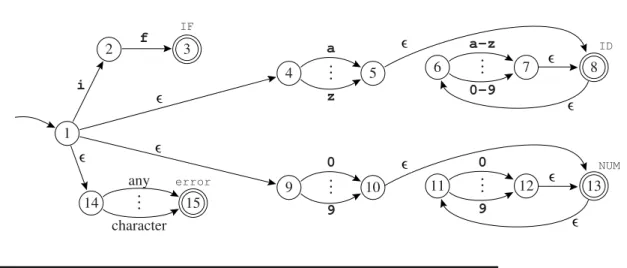
Figure 2.6 shows the rules for translating regular expressions to nondeterministic automata. We illustrate the algorithm on some of the expressions inFigure 2.2 – for the tokens IF, ID, NUM, and error. Each expression is translated to an NFA, the “head” state of each NFA is marked final with a different token type, and the tails of all the expressions are joined to a new start node. The result – after some merging of equivalent NFA states – is shown in Figure 2.7.

(38)

1

any character

3

2 f ^IF

5 z a

4 .

..

0-9 a-z

6 .

..

ID

10 9 0

9 .

..

9 0 11

7

. 12

..

NUM

14 .

..

error

15 i

8

13

FIGURE 2.7. Four regular expressions translated to an NFA.

CONVERTING AN NFA TO A DFA

As we saw inSection 2.3, implementing deterministic finite automata (DFAs) as computer programs is easy. But implementing NFAs is a bit harder, since most computers don’t have good “guessing” hardware.

We can avoid the need to guess by trying every possibility at once. Let us simulate the NFA ofFigure 2.7on the stringin. We start in state 1. Now, instead of guessing which ϵ-transition to take, we just say that at this point the NFA might take any of them, so it is in one of the states {1, 4, 9, 14}; that is, we compute the ϵ-closure of {1}. Clearly, there are no other states reachable without eating the first character of the input.

Now, we make the transition on the characteri. From state 1 we can reach 2, from 4 we reach 5, from 9 we go nowhere, and from 14 we reach 15. So we have the set {2, 5, 15}. But again we must compute ϵ-closure: from 5 there is an ϵ-transition to 8, and from 8 to 6. So the NFA must be in one of the states {2, 5, 6, 8, 15}.

On the charactern, we get from state 6 to 7, from 2 to nowhere, from 5 to nowhere, from 8 to nowhere, and from 15 to nowhere. So we have the set {7};

its ϵ-closure is {6, 7, 8}.

Now we are at the end of the string in; is the NFA in a final state? One of the states in our possible-states set is 8, which is final. Thus, inis an ID

token.

We formally define ϵ-closure as follows. Let edge(s, c) be the set of all NFA states reachable by following a single edge with label c from state s.

(39)

For a set of states S, closure(S) is the set of states that can be reached from a state in S without consuming any of the input, that is, by going only through ϵ edges. Mathematically, we can express the idea of going through ϵ edges by saying that closure(S) is smallest set T such that

T = S ∪

!

"

s∈T

edge(s, ϵ)

# . We can calculate T by iteration:

T ← S repeat T^′←T

T ← T^′∪ ($

s∈T^′edge(s, ϵ)) until T = T^′

Why does this algorithm work? T can only grow in each iteration, so the final T must include S. If T = T^′after an iteration step, then T must also in- clude $_s∈T′edge(s, ϵ). Finally, the algorithm must terminate, because there are only a finite number of distinct states in the NFA.

Now, when simulating an NFA as described above, suppose we are in a set d = {s_i,s_k,s_l}of NFA states s_i,s_k,s_l. By starting in d and eating the input symbol c, we reach a new set of NFA states; we’ll call this set DFAedge(d, c):

DFAedge(d, c) = closure("

s∈d

edge(s, c))

Using DFAedge, we can write the NFA simulation algorithm more formally.

If the start state of the NFA is s₁, and the input string is c₁, . . . ,c_k, then the algorithm is:

d ←closure({s1}) for i ← 1 to k

d ← DFAedge(d, c_i)

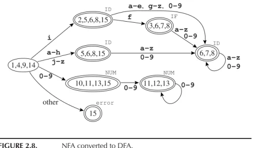
Manipulating sets of states is expensive – too costly to want to do on every character in the source program that is being lexically analyzed. But it is possible to do all the sets-of-states calculations in advance. We make a DFA from the NFA, such that each set of NFA states corresponds to one DFA state.

Since the NFA has a finite number n of states, the DFA will also have a finite number (at most 2ⁿ) of states.

DFA construction is easy once we have closure and DFAedge algorithms.

The DFA start state d₁ is just closure(s₁), as in the NFA simulation algo-

(40)

a-h j-z

IF ID

NUM

error

i

1,4,9,14

2,5,6,8,15

5,6,8,15

10,11,13,15

6,7,8

11,12,13

15 0-9

f

a-z 0-9

other

0-9

ID

NUM

a-z 0-9 0-9

ID

3,6,7,8 a-e, g-z, 0-9

FIGURE 2.8. NFA converted to DFA.

rithm. Abstractly, there is an edge from d_i to d_j labeled with c if d_j = DFAedge(d_i,c). We let $ be the alphabet.

states[0] ← {}; states[1] ← closure({s1}) p ←1; j ←0

while j ≤ p foreach c ∈ $

e ←DFAedge(states[ j], c) if e = states[i] for some i ≤ p

then trans[ j, c] ← i else p ← p + 1

states[ p] ← e trans[ j, c] ← p j ← j +1

The algorithm does not visit unreachable states of the DFA. This is ex- tremely important, because in principle the DFA has 2ⁿstates, but in practice we usually find that only about n of them are reachable from the start state.

It is important to avoid an exponential blowup in the size of the DFA interpreter’s transition tables, which will form part of the working compiler.

A state d is final in the DFA if any NFA-state in states[d] is final in the NFA. Labeling a state final is not enough; we must also say what token is recognized; and perhaps several members of states[d] are final in the NFA.

In this case we label d with the token-type that occurred first in the list of