形式化驗證零知識證明系統編譯器

(1)

國立臺灣大學電機資訊學院電機工程學系碩士論文

Department of Electrical Engineering

College of Electrical Engineering and Computer Science

National Taiwan University Master Thesis

形式化驗證零知識證明系統編譯器

From a Dependently Typed Language to ZK-SNARKs Circuits: A Formally Verified Compiler

許瑞麟 Ruey-Lin Hsu

指導教授：鄭振牟博士

Advisor: Chen-Mou Cheng, Ph.D.

中華民國 109 年 7 月 July, 2020

(2)

(3)

謝

首先，我要感謝我的指導教授鄭振牟教授，是他指引了我進入了密碼學相關的領域，也是他向說我提出了此論文的零知識證明題目。再來，我要感謝穆信成研究員，是他使我了解了許多與型別理論，程式推導，和許多與程式語言理論有關的東西。並且，穆老師也對我的論文提出了很多有幫助的意見。另外，我要感謝我的口試委員：鄭振牟，

楊伯因，穆信成，柯向上，謝謝他們願意撥出時間來當我的口試委員以及參加我的口試。

(4)

(5)

Acknowledgements

Above all, I want to thank my advisor Professor Chen-Mou Cheng for what he did to introduce me to the field of cryptography and proposed the topic for this dependently typed zkSNARK compiler to me. I also want to thank Researcher Shin-Cheng Mu who helped me understand many programming language theory related topics like type theory and program derivation, and gave a lot of helpful comments regarding my master thesis. Further- more, I want to thank Chen-Mou Cheng, Bo-Ying Yang, Shin-Cheng Mu, and Hsiang-Shang Ko for being a part of my oral examination committee and taking the time to participate in my oral examination.

(6)

(7)

要

本論文提出一個依值型別的可驗證計算編譯器，並證明其可靠性。

此編譯器將一個淺層嵌入於 Agda 當中，具有依值型別的領域特定語言轉換成一階限制條件。可靠性是轉換正確性的一個部份，表示如果產生出來的限制條件是可被滿足的，那產生出來的限制條件會是正確的。藉由利用柯里-霍華德對應，我們在互動式定理證明器 Agda 當中建構此編譯器的形式規格以及證明其可靠性。

關：依值型別程式設計, 互動式定理證明器, 可驗證計算, 形式化

驗證, Agda

(8)

(9)

Abstract

In this thesis, we will construct and prove the soundness of a dependently typed verifiable computation compiler. The compiler described in this thesis compiles a user program written in a dependently typed shallowly embedded domain specific language in Agda into a set of rank 1 constraints. Soundness is a part of translational correctness that says that if the generated constraints are satisfiable, then the generated constraints are correct. By utilizing the Curry-Howard correspondence, the compiler is formally specified and proved in the interactive theorem prover Agda.

Keywords: dependently typed programming, interactive theorem prover, verifiable computation, formal verification, Agda

(10)

(11)

List of Figures

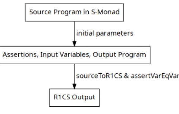
1.1 Compilation Pipeline . . . 1

(14)

(15)

Chapter 1 Introduction

Dependent type theory[11] is a powerful general purpose tool that can be used for both general purpose programming and theorem proving. One of the most fascinating and powerful things about interactive proof assistants based on dependent type theories like Agda[13], Coq[15], and Idris[4] is the abilily to develop programs together with speci- fications and proofs of their properties in the same language through the Curry-Howard correspondence.

In this thesis, I will describe the construction and formal verification of a verifiable computation compiler that compiles a dependently typed EDSL (embedded domain specific language) in Agda into a set of rank 1 constraints, which is then piped into the zk- SNARK library libsnark.

Figure 1.1: Compilation Pipeline

This thesis is an attempt at integrating dependently typed programming into verifi-

(16)

able computation schemes. A verifiable computation scheme can be used to outsource a computation to a potentially untrusted third party, where one only has to examine a small cryptographic proof to know that the computation is performed correctly by a third party.

One way of thinking about type systems in programming languages is that type systems are a way of statically eliminating incorrect programs that might go wrong when executed.

Another way to think about type systems in programming languages is that a type tells you what you can expect from a program. Suppose that a program p has type (Int, Int), then the programmer might expect a tuple of integers from the execution of p instead of say, a tuple of strings.

The work of Steward et al.[14] on verifiable computation lets a person write declarative programs living in a Haskell DSL that compiles to verifiable computation constraints.

Logically one might think that since dependently typed programming has a long history in interactive theorem proving and functional programming, it would be interesting to see what it is like to have a DSL with a more expressive type system that can compile to verifiable computation constraints. This work is an attempt to explore this question with dependently typed programming.

By using inductive-recursive definitions to encode dependent types à la Tarski[6], it is possible to embed a dependently typed DSL within a dependently typed language itself.

This type encoding construction is then used to construct a dependently typed Agda DSL that targets the verifiable computation backend R1CS. One thing that having dependent type allows us to have is branching. Having dependent types in our language allows us to express the possibility of executing different programs with distinct types within our DSL.

The embedded Agda DSL used for composing the source programs is designed to be used together with a state transformation monad that records an unused variable together with a list of input variables (natural numbers) and a list of solver hints and equality constraints over an inductively defined Source datatype (indexed over the type of type codes representing permitted types).

Chapter 2 introduces the background knowledge and ideas used in the compiler, such

(17)

as type theory, zkSNARK, and verifiable computing. Chapter 3 describes the basic con- structions used in the compiler. Chapter 4 describes the source language and the utilities that can be used when writing programs in the source language. In Chapter 5, the construction of the verifiable computation compiler is described, and in Chapter 6, the formal verification of the soundness of the compiler is described.

(18)

(19)

Chapter 2 Background

2.1 Type Theory

Dependent type theory a la MLTT is a Gentzen style natural deduction system. A derivation in such a system can be seen as an annotated proof tree, and a program can be seen as a microcosm of its corresponding proof tree. Type theory naturally gives rise to the Curry- Howard correspondence: the propositions as types interpretation tells us that a program corresponds to a proof and a type corresponds to a proposition.

The Π type represents universal quantification:

Γ⊢ A : Set Γ⊢ B : A → Set Π-F Γ⊢ Πx : AB x : Set

Γ, x : A⊢ t : B x

Π-I Γ⊢ λx : A. t : Πx : AB x

Γ⊢ t1 : Π_{x : A}B x Γ⊢ t2 : A Π-E Γ⊢ t1t₂: B t₂

The Σ type represents existential quantification:

(20)

Γ⊢ A : Set Γ⊢ B : A → Set Σ-F Γ⊢ Σx : AB x : Set

Γ⊢ t1 : A Γ⊢ t2 : B t1

Σ-I Γ⊢ (t1, t₂) : Σ_{x : A} B x

Γ⊢ p : Σx : AB x Σ-fst Γ⊢ fst p : A

Γ⊢ p : Σx : AB x

Σ-snd Γ⊢ snd p : B (fst p)

Non-dependent logical implication and cartesian product are special cases of Π and Σ types respectively.

In type theory, there is the notion of definitional equality, which is a meta-theoretic equality, and which forms the basis of type checking. Terms and types that are definitionally equal are indistinguishable on the object level. Definitional equality can be defined as the equivalence relation generated by a set of structural and equivalence closure rules stating that equal terms are substitutable everywhere and that terms are definitionally iden- tified up to β conversion.

There is also the notion of propositional equality (or equality type), which is an object level equality that expresses the fact that two terms are equal:

Γ⊢ A : Set

≡-F Γ⊢ _≡A_ : A→ A → Set

Γ⊢ x : A

≡-I Γ⊢ refl x : x ≡Ax

(21)

Γ⊢ C : (x y : A) → x ≡Ay→ Set Γ⊢ C-refl : (x : A) → C x x (refl x) Γ⊢ x : A

Γ⊢ y : A Γ⊢ p : x ≡Ay

≡-E(J) Γ⊢ ≡-ind C C-refl x y p : C x y p

In Agda, the Σ type and the propositional equality type can be roughly translated into their corresponding datatype definitions:

record Σ (A : Set) (B : A → Set) : Set where constructor _,_

field fst : A snd : B fst

data _≡_ {A : Set} : A → A → Set where refl : (x : A) → x ≡ x

and a Π type corresponds to a function definition in Agda.

Proofs in Agda are written with dependent pattern matching, which was shown to be equivalent to traditional type theory with inductive families plus the addition of axiom K[9][12]. Recent work [5] has also shown that by placing certain restrictions on dependent pattern matching, it’s possible to translate programs written with restricted pattern matching rules into traditional type theory with inductive families without the use of axiom K. However, in this thesis, we will be using axiom K to construct the compiler and prove its soundness.

2.2 Verifiable Computation

Verifiable computation can be used to delegate computations to potentially untrusted ma- chines. In this thesis we will focus on a particular approach of verifiable computation –

(22)

zkSNARKs. Currently, there are a couple of potential applications for zkSNARKs, like private transactions or smart contracts in cryptocurrencies and verifiable computation. In a zkSNARK, there are two parties, a prover and a verifier. The prover is the party per- forming the computation, and the one producing a cryptographic proof π that the verifier can use to determine with high probability whether or not the computation is performed correctly.

A zkSNARK consists of a set of probabilistic algorithms: KeyGen (K), Prove (P), and Verify (V). Given a security parameter λ and a program C, a zkSNARK protocol goes as follows:

(k_p, k_v)← K(λ, C)

π ← P(C, kp, public, witness) {true, false} ← V(C, kv, public, π)

where k_p is the proving key, k_v is the verifcation key, public is the public variables, witness is the non-public (private) variables, andC is the program.

In this thesis, the programC fed to the keygen, the prover and the verifier will be the R1CS constraints (defined below) generated by our compiler. The variables inC include the input and output variables of the program together with all the intermediate values.

And public together with witness constitute the variables inC (the purpose of witness will be discussed later in this section).

Definition 2.2.1. A rank 1 constraint system[2] (R1CS) S over a field F with Ng con- straints is a set of vectors

{(ai, b_i, c_i)|i ∈ [1, Ng], a_i ∈ F^1+N^v, b_i ∈ F^1+N^v, c_i ∈ F^1+N^v}.

and a non-negative integer N_i, where

• F is a field

(23)

• Nv is the number of variables

• N_i ≤ Nv is the number of public variables.

If there is some public values x∈ F^Nⁱ and private values (witness) w ∈ F^N^v^−Nⁱ such that

⟨ai, (1, x, w)⟩⟨bi, (1, x, w)⟩ = ⟨ci, (1, x, w)⟩

for all i∈ [1, Ng] (where⟨m, n⟩ denotes the dot product of m and n, and the left hand side of the equation multiplies the two dot products together), then S is said to be satisfiable with public values x and witness w.

The definition of R1CS can be seen as a charaterization of NP problems as NP-complete problems like SAT can be reduced to R1CS satisfaction problems in polynomial time, and this is used to define what it means to “know” something in the zkSNARK proof of knowledge definition.

Suppose that a programmer A has written a program P rog(a, b) = (a + b)∗ b where a, b ∈ F are the inputs to P rog and A wants to outsource this computation P rog to an untrusted cloud server CS. A can choose to encode P rog as R1CS constraints (which can then be further processed into a quadratic arithmetic program (QAP)[8]).

In this example, P rog can be encoded with a single R1CS constraint with three R1CS variables. Besides a and b, we need another variable out to represent the output of the program, that is, out = (a + b)∗ b. So if we fix the order of the variables (including the constant 1) to be [1, a, b, out], the R1CS constraint would be a singleton set consisting of the element ([0, 1, 1, 0], [0, 0, 1, 0], [0, 0, 0, 1]). What if we require a to be a boolean?

This can be accomplised by adding another constraint ([0, 1, 0, 0], [0, 1, 0, 0], [0, 1, 0, 0]) (which says that a² = a) to the set of constraints. If a is equal to 0, this constraint is satisfied. Otherwise, if a ̸= 0, we multiple both sides of the equation by a⁻¹, and we get that it must be the case that a = 1, and thus, a is a boolean. In this scenario, A wants to know the result out, and the three variables a, b, and out are all public variable in the zkSNARK.

After the program is encoded into R1CS, the resulting constraints are then sent to CS,

(24)

where a key pair is first generated by A and then the programmer has to decide the input to be fed into P rog (say, fixing a = 2 and b = 3).

Then the transformed arithmetic constraints along with the fixed inputs 2 and 3 are then sent to CS (which will then try to solve the variable out in the transformed constraints and execute the prover algorithmP with a, b, and out to generate the proof π). CS then gives π and the variables that are considered to be public to A (which plays the role of the verifier). A then checks if the combination of the public variables and π is valid, and if it is valid, then A can have a high confidence that CS has indeed performed the required computations, and that the output is correct provided that the transformation of P rog is correct.

In some variants of the above scenario, the prover might want to hide some information from the verifier, and this is where the private witness in S comes into play. For example, the prover might want to hide the intermediate values resulting from the execution of a program from the verifier (and only the input and output of the program is made public), and from the zero knowledge guarantee from the zk-SNARK backend, we can know that apart from the public variables, the proof π doesn’t tell us additional information about the private witness in V C. The properties that a zkSNARK system has to satisfy is made more precise in the following paragraph.

A zkSNARK[2][3] (which stands for zero knowledge succinct non-interactive argument of knowledge) satisfies the following properties:

• completeness: If public together with witness constitutes a solution to a program C, and

(kp, kv)← K(λ, C)

π ← P(C, kp, public, witness)

then

V(C, kv, public, π) = true.

(25)

• succintness: the size of the proof π generated by P is Oλ(1) (independent of the size of C).

• proof of knowledge: For any probabilistic polynomial time (PPT) adversary A, there is a PPT extractor E such that for every constant c > 0, large enough λ, auxiliary input z (where|z| = poly(λ)) and every program C of size λ^c,

Pr







V(C, kv, public, π) = true (public, witness) not a solution ofC

(k_p, k_v) ← K(λ, C) (public, π) ← A(z, pk, p_v) witness ← E(z, pk, p_v, r_A)







≤ negl(λ)

where r_Ais the random tape of A.

• zero knowledge: meaning that the proof π does not leak any information about witness.

Completeness says that someone with a solution (public, witness) to a program C can always produce a proof π that convinces a verifier who follows the zkSNARK protocol.

Sunccinctness says that the proof π is small. Proof of knowledge says that if a PPT ad- versary produces public and a proof π thatV checks to be valid, then with a large enough λ, there is a high probability that there is a PPT knowledge extractor E that can “extract”

the knowledge witness from A so that (public, witness) is a solution toC.

Since we will be building the constraints in Agda, following the work of Stewart et al[14], we define the target compilation type R1CS as follows (parameterized over a type f):

data R1CS : Set where

IAdd : f → List (f × Var) → R1CS -- sums to zero

IMul : (a : f) → (b : Var) → (c : Var)

→ (d : f) → (e : Var) → R1CS

(26)

-- a * b * c = d * e

Hint : (Map Var ℕ → Map Var ℕ) → R1CS Log : String → R1CS

where IAdd f1 ((f2, i2) ∷ (f3, i3) ... ∷ []) expresses an additive constraint f1 + f2vi2 + f₃v_i₃... = 0, f_i ∈ F, vik ∈ F, and IMul fa b c f_d e expresses a multiplicative constraint f_av_bv_c = f_dv_ewhere f_a, v_b, b_c, f_d, v_e ∈ F. The vectors in an R1CS constraint system are usually sparse and this is why the R1CS datatype is not defined as a tuple of vectors. A list of constraints of type [R1CS] in Agda can be easily transformed into the regular tuple of vectors representation. Since a set of R1CS constraints represents an NP-complete problem in general, the definition of R1CS includes hints to help the solver solve these R1CS constraints (and also Log to help with debugging).

To date, there have been numerous attempts at compiling existing programming languages like C, or specially designed domain specific languages into zkSNARK systems.

ZoKrates[16], SNARKs for C[2], Snårkl[14], and the formally verified compiler made by Fournet et al[7] are all examples of this. However, the source languages of these existing compilers lack an expressive type system. Inspired by the work of Snårkl, we attempt to construct and integrate a dependently typed embedded domain specific language into a verifiable computation system.

(27)

Chapter 3 Constructing an Embedded Type Universe

In this chapter, we are going to construct a dependently typed embedded type universe and determine R1CS variable allocation for an element in our embedded type universe. First we are going to describe how the embedded type universe is constructed for our EDSL.

The constructed type universe will have the property that each type in the type universe will only have finitely many inhabitants (when instantiated with a finite base type). For such instantiations of our type universe, we can construct an enumeration function enum that enumerates elements for any embedded type u such that every element in enum u only appears once.

Given a function occ that counts the number of occurrences of a given element in a list and a comparison function dec that tells us whether or not two elements with type u are equal, the fact that every element in enum u is unique can be expressed as follows: for any element val with type u, occ dec val (enum u) ≡ 1.

Towards the end of this chapter, we will prove that this proposition indeed holds for all type code u, and we will show how enum can be used to determine the number of R1CS variables that will be allocated in the compilation process for an element of type u.

(28)

3.1 Type Code

In this section, we are going to define the main datatype for the embedded type codes.

Type codes are used to define the types that are allowed in the embedded DSL and is defined as an inductive-recursive definition[6] in Agda. Given any type f, the type codes are defined in an Agda module parameterized over f as follows:

Definition 3.1.1 (Type Code).

data U : Set

⟦_⟧ : U → Set

data U where

`One : U

`Two : U

`Base : U

`Vec : (S : U) → ℕ → U

`Σ `Π : (S : U) → (⟦ S ⟧ → U) → U

⟦ `One ⟧ = ⊤

⟦ `Two ⟧ = Bool

⟦ `Base ⟧ = f

⟦ `Vec ty x ⟧ = Vec ⟦ ty ⟧ x

⟦ `Σ fst snd ⟧ = Σ ⟦ fst ⟧ (λ f → ⟦ snd f ⟧)

⟦ `Π fst snd ⟧ = (x : ⟦ fst ⟧) → ⟦ snd x ⟧

By interpreting the type codes in U through⟦_⟧, a subset of Agda types that are allowed in our EDSL can be obtained. In this thesis, we will instantiate f with types that represent finite fields since we will be compiling the EDSL into finite field constraints. Later on in this section we are going to define what it means for a type together with a set of operators to be a finite field.

(29)

For example, suppose that we have an Agda function fromBits : {n : ℕ} → Vec Bool n →ℕ that transforms an n bit-encoded number into ℕ, then the type code ‘Σ ‘Two (λ x₁

→ ‘Σ ‘Two (λ x₂ → ... ‘Σ ‘Two (λ xₙ → ‘Vec ‘Base (fromBits (x₁ ∷ x₂ ∷ ... ∷ xₙ ∷ []))))) expresses the type of vectors with their lengths encoded in n bits. Similarly, we can have matrices with the number of rows and columns encoded in m + n bits respectively.

Intuitively, one can see that if the type f has only finitely many inhabitants, then for any u : U,⟦ u ⟧ also only has finitely many inhabitants, and as such, it is possible to obtain an enumeration of the elements in⟦ u ⟧. Formally, we define a type A to be finite or have finitely many inhabitants if there is an enumeration l : List A of elements in A such that for any x : A, x∈ l and that any x in l only occurs once in l. We now define the pieces (list membership and element counting) that will be put together to form the definition of our finite type in Agda.

3.2 List Membership

Definition 3.2.1 (Any).

data Any {A : Set} (P : A → Set) : List A → Set where

here : ∀ {x xs} (px : P x) → Any P (x ∷ xs) there : ∀ {x xs} (pxs : Any P xs) → Any P (x ∷ xs)

Given a predicate P : A → Set and a list l : List A, Any P l holds if there is at least one element m : A in l such that P m holds.

With the Any datatype defined, we now proceed to define the membership relation.

Given a type A together with an equivalence relation _≈_, the membership relation is defined as follows:

Definition 3.2.2 (_∈_).

_∈_ : A → List A → Set x ∈ xs = Any (x ≈_) xs

Unless otherwise explicitly stated, _∈_ will be used with propositional equality.

(30)

3.3 Counting Number of Occurrences

When proving the soundness of the compiler, some of the steps require us to prove that elements in enum u are unique. To facilitate the development of such proofs (and to define what it means for a type to have finitely many inhabitants), we define a function occ that counts the number of occurrences of an element in a list.

Defining occ requires us to have the ability to determine whether or not propositional equality holds between two inhabitants of a specific type. This is captured with the following definitions:

Definition 3.3.1 (Dec). Decidability of a proposition P

data Dec (P : Set) : Set where yes : (p : P) → Dec P

no : (¬p : ¬ P) → Dec P

Dec P holds if either P is true or¬ P is true.

Definition 3.3.2 (Decidable).

Decidable : {A B : Set} → (A → B → Set) → Set Decidable _∼_ = ∀ x y → Dec (x ∼ y)

If Decidable holds for some equality _~_ : A → A → Set, this means that for any elements x y : A, we can decide whether or not x and y are propositionally equal.

Equipped with the definition of Decidable, occ is defined as follows.

Definition 3.3.3 (occ). Number of times an element appears in a list (up to propositional

equality).

occ : ∀ {A : Set}

→ (Decidable {A = A} _≡_) → A → List A → ℕ occ dec a [] = 0

occ dec a (x ∷ l) with dec a x ... | yes p = suc (occ dec a l) ... | no ¬p = occ dec a l

(31)

With list membership and element counting defined, we now define Finite in the fol- lowing section.

3.4 Finite Types

Given a typef : Set, the predicate Finite is defined as an enumeration of all elements of f such that any inhabitant of f only appears in the enumeration once (up to propositional equality).

Definition 3.4.1 (Finite).

record Finite (f : Set) : Set where field

elems : List f size : ℕ

a∈elems : (a : f) → a ∈ elems

occ-1 : (a : f) (dec : Decidable _≡_)

→ occ dec a elems ≡ 1

size≡len-elems : size ≡ length elems

Note that given an arbitrary type f and a b : Finite f, it is not necessarily the case that a ≡_{Finite f}b since the enumeration in a can be a permutation of the enumeration in b.

Our target compilation type R1CS comprises prime field elements and variables. After Finite is defined, we now define what it means for a type to be an algebraic field.

3.5 Field

Definition 3.5.1 (Field). Field f is defined as a record consisting of an addition operator _+_, a multiplication operator _*_, an additive unit zero, a multiplicative unit one, an additive inverse operation -_, and a multiplicative inverse 1/_.

record Field (f : Set) : Set where field

(32)

_+_ _*_ : f → f → f -_ : f → f

1/_ : f → f zero : f one : f

(Note: _+_, _*_, -_, 1/_, zero, one are renamed to be _+F_, _*F_, -F_, 1F/_, zerof, onef respectively in the later chapters of this thesis)

Definition 3.5.2 (IsField). Field axioms.

record IsField (f : Set) (field' : Field f) : Set where

open Field field' field

+-identityˡ : ∀ x → zero + x ≡ x +-identityʳ : ∀ x → x + zero ≡ x +-comm : ∀ x y → x + y ≡ y + x

*-comm : ∀ x y → x * y ≡ y * x

*-identityˡ : ∀ x → one * x ≡ x

*-identityʳ : ∀ x → x * one ≡ x +-assoc : ∀ x y z → ((x + y) + z)

≡ (x + (y + z))

*-assoc : ∀ x y z → ((x * y) * z)

≡ (x * (y * z)) +-invˡ : ∀ x → ((- x) + x) ≡ zero

+-invʳ : ∀ x → (x + (- x)) ≡ zero

*-invˡ : ∀ x → ¬ x ≡ zero → (1/ x) * x ≡ one

*-invʳ : ∀ x → ¬ x ≡ zero → x * (1/ x) ≡ one

*-distr-+ˡ : ∀ x y z → (x * (y + z))

≡ ((x * y) + (x * z))

(33)

*-distr-+ʳ : ∀ x y z → ((y + z) * x)

≡ ((y * x) + (z * x))

IsField f ops describes the conditions for a type f with the field operations ops to be a field.

With our embedded type universe and the definition of finite field defined, we now proceed to define list monad before we construct the enumeration function enum that enu- merates elements of⟦ u ⟧.

3.6 List Monad

Definition 3.6.1 (return). (List)

return : ∀ {A : Set} → A → List A return a = [ a ]

where [ a ] denotes the singleton list with only one element a in it.

Definition 3.6.2 (_>>=_). (List)

_>>=_ : {A B : Set}

→ List A → (A → List B) → List B [] >>= f = []

(x ∷ ma) >>= f = f x ++ (ma >>= f)

where ++ denotes list concatenation.

In order to reason about monadic programs written in list monad later on, we prove a couple of lemmas to fascilitate these proofs.

3.6.1 Properties of List Monad

Suppose that we have l >>= f : List A for some A. What is a necessary and sufficient condition for us to know that a particular element y falls inside of l >>= f ? If there is an element x∈ l such that y ∈ f x, then we know that it must also fall inside of l >>= f :

(34)

Lemma 3.6.1 (∈->>=).

∈->>= : ∀ {A B : Set} (l : List A) (f : A → List B) → ∀ x → x ∈ l

→ ∀ y → y ∈ f x → y ∈ l >>= f

Proof. By straightforward induction on the derivation of x∈ l.

Conversely, we have:

Lemma 3.6.2 (∈->>=⁻).

∈->>=⁻ : {A B : Set} (l : List A)

(f : A → List B) → ∀ y → y ∈ l >>= f

→ ∃ (λ x → x ∈ l × y ∈ f x)

Proof. By straightforward induction on l.

Now suppose that we’ve written the following Agda program to help with enumerating elements of some finite types A and B:

makeProducts : {A B : Set}

→ List A → List B → List (A × B) makeProducts l₁ l₂ = do

a ← l₁ b ← l₂

return (a , b)

where _×_ denotes the usual cartesian product type. It’s obvious that an element (x, y) : A × B falls inside of makeProducts l₁ l₂ when x ∈ l₁ and y ∈ l₂. The following lemma proves a generalized version of the above statement where B is dependent on A and the domain of _+_ ranges over arbitrary (m : A) and (n : B m).

Lemma 3.6.3 (∈l-∈l’-∈r).

(35)

∈l-∈l'-∈r : ∀ {A : Set} {B : A → Set} {C : Set}

(l : List A) (_+_ : (x : A) → B x → C)

→ ∀ x y → x ∈ l → (l' : (x : A) → List (B x))

→ y ∈ l' x → x + y ∈ (l >>= λ r → l' r >>= λ rs → return (r + rs))

Proof. Corollary of∈->>=.

In the later sections of this chapter, we are going to prove that elements in the enu- meration produced by enum (which will be introduced later in this chapter) are unique.

The following lemma is going to help with decomposing the number of occurrences of an element in the subparts of enum into simpler parts. Take the program makeProducts in Section 3.6.1 for example again, if every element of l₁ in makeProducts is unique, then the proposition∀ x₁ → ¬ x ≡ x₁ → ¬ y ∈ f x₁ (a premise of occ->>=) is satisfied for any x

∈ l₁ : List A and k : B such that y = (x, k) and f = λ a → l₂ >>= λ b → (a , b) (because the first projections of the tuples are distinct). And the following lemma is going to be applied when we are counting occurrences of elements that appear in the subparts of enum, which are constructed in a way that is similar to the above makeProducts example.

Lemma 3.6.4 (occ->>=).

occ->>= : ∀ {A B : Set}

(decA : Decidable {A = A} _≡_) (decB : Decidable {B = B} _≡_)

(l : List A) (f : A → List B) → ∀ x y → (prf : ∀ x₁ → ¬ x ≡ x₁ → ¬ y ∈ f x₁) →

occ decB y (l >>= f) ≡ (occ decA x l * occ decB y (f x))

As the embedded DSL is compiled into R1CS, it is necessary to determine the R1CS representation of an element e : ⟦ u ⟧. To achieve this, the number of variables that has

(36)

to be allocated for e has to be determined. Before we define the function tySize that de- termines how many variables are allocated for an element of some⟦ u ⟧, the enumeration function enum that enumerates elements of embedded types is defined first as we rely on enum to determine R1CS variable allocation.

3.7 Enumerating Elements of Embedded Types

For any finite type f, it is possible to define an enumeration function enum : (u : U) → List⟦ u ⟧ that enumerates all elements of ⟦ u ⟧ exactly once for all u since the base cases are finite. Most cases of enum are quite trivial. The only non-trivial case is the case of Π types.

3.7.1 Enumerating Elements of Embedded Pi Types

In order to enumerate elements of embedded Π types, a couple of auxiliary definitions are needed. Observe that when pattern matching is done on u, in the case of Π types (let u =

‘Π v x), it is easy to generate a list of pairs of type List (Σ⟦ v ⟧ (λ k → List ⟦ x k ⟧)) with the usual list monad by structural recursion that pairs possible inputs to the Π type with the possible outputs together:

pairs = enum v >>= \r -> return (r , enum (x r))

With these pairs defined, we now define a function genFunc that transforms these pairs into List (List (Σ⟦ u ⟧ (λ v → ⟦ x v ⟧))) (which represents a list of functions) that can then be further transformed into a list of functions:

Definition 3.7.1 (genFunc).

genFunc : ∀ (u : U) (x : ⟦ u ⟧ → U)

→ List (Σ ⟦ u ⟧ (λ v → List ⟦ x v ⟧))

→ List (List (Σ ⟦ u ⟧ (λ v → ⟦ x v ⟧))) genFunc u x [] = [ [] ]

genFunc u x (x₁ ∷ l) with genFunc u x l

(37)

... | rec = do r ← rec

choice ← proj₂ x₁

return ((proj₁ x₁ , choice) ∷ r)

To give a sense of what genFunc is doing, suppose that we are given a constant type family fam over ‘Two that maps false and true to ‘Base¹, and the list l = [(false , [2, 3]), (true , [5, 6])] of type List (Σ⟦ ‘Two ⟧ (λ v → List ⟦ fam v ⟧)). This input list says that the functions that we are building can map false to either 2 or 3, and map true to either 5 or 6.

By feeding these arguments into genFunc, we get the list of all possible input output pairs [[(false, 2), (true, 5)], [(false, 3), (true, 5)], [(false, 2), (true, 6)], [(false, 3), (true, 6)]].

The relationship between the elements in the output of genFunc and the input list of genFunc is captured by the following relation:

Definition 3.7.2 (FuncInst).

data FuncInst (A : Set) (B : A → Set)

: List (Σ A B) → List (Σ A (λ v → List (B v)))

→ Set where

InstNil : FuncInst A B [] []

InstCons : ∀ l l' → (a : A) (b : B a) (ls : List (B a))

→ b ∈ ls → (ins : FuncInst A B l l')

→ FuncInst A B ((a , b) ∷ l) ((a , ls) ∷ l')

An instance of FuncInst A B xs ys says that if x and y are the i-th elements of xs and ys respectively, then proj₁ x and proj₁y are equal, and proj₂ x∈ proj2y.

We show that FuncInst ⟦ u ⟧ (λ z → ⟦ x z ⟧) f l if and only if f ∈ genFunc u x l with the following two lemmas.

Lemma 3.7.1 (FuncInst→genFunc).

1where ‘Base maps to say a prime field or natural numbers

(38)

FuncInst→genFunc : ∀ (u : U) (x : ⟦ u ⟧ → U) (l : List (Σ ⟦ u ⟧ (λ v → List ⟦ x v ⟧))) (f : List (Σ ⟦ u ⟧ (λ v → ⟦ x v ⟧)))

→ FuncInst ⟦ u ⟧ (λ z → ⟦ x z ⟧) f l

→ f ∈ genFunc u x l

Proof. By induction on the derivation of FuncInst. The base case is trivial, and the induc- tive case is proved by straightforward application of∈->>=.

Lemma 3.7.2 (genFunc→FuncInst).

genFunc→FuncInst : ∀ (u : U) (x : ⟦ u ⟧ → U) (l : List (Σ ⟦ u ⟧ (λ v → List ⟦ x v ⟧))) (f : List (Σ ⟦ u ⟧ (λ v → ⟦ x v ⟧)))

→ f ∈ genFunc u x l

→ FuncInst ⟦ u ⟧ (λ z → ⟦ x z ⟧) f l

Proof. By induction on l.

genFunc also satisfies this property (which is captured by FuncInst):

Lemma 3.7.3 (genFuncProj₁).

genFuncProj₁ : ∀ (u : U) (x : ⟦ u ⟧ → U)

→ (l : List (Σ ⟦ u ⟧ (λ v → List ⟦ x v ⟧)))

→ (x₁ : List (Σ ⟦ u ⟧ (λ v → ⟦ x v ⟧)))

→ x₁ ∈ genFunc u x l

→ map proj₁ x₁ ≡ map proj₁ l

Proof. By induction on l. The base case is trivial, and the inductive case can be proved with∈->>=⁻ and IH.

After genFunc is defined, we need to construct a function that transforms the output of genFunc into a list of actual functions. To do this, we first construct the following piFromList function that transforms a list of input output pairs into a partial function (from (dom : ⟦ u ⟧) to ⟦ x dom ⟧) by induction on the derivation of dom ∈ enough:

(39)

Definition 3.7.3 (piFromList).

piFromList : ∀ (u : U) (x : ⟦ u ⟧ → U)

→ (enough : List ⟦ u ⟧)

→ (l : List (Σ ⟦ u ⟧ (λ v → ⟦ x v ⟧)))

→ (map proj₁ l ≡ enough)

→ (dom : ⟦ u ⟧)

→ dom ∈ enough → ⟦ x dom ⟧

piFromList u x .(d ∷ _) ((d , v) ∷ l) refl dom (here refl) = v

piFromList u x (._ ∷ rest) (x₁ ∷ l) refl dom (there dom∈enough)

= piFromList u x rest l refl dom dom∈enough

and provided with a proof∀ x → x ∈ eu that the enumeration of u is complete, we can get total functions out of piFromList as demonstrated in the following listFuncToPi function when the inputs are in sync. When listFuncToPi is given a list l : List (List (Σ⟦ u ⟧ (λ v

→⟦ x v ⟧))) representing a list of Π functions, we can get a list of actual functions as its output (given that l is good enough):

Definition 3.7.4 (listFuncToPi).

listFuncToPi : ∀ (u : U) (x : ⟦ u ⟧ → U)

→ (eu : List ⟦ u ⟧)

→ (∀ elem → elem ∈ eu)

→ (l : List (List (Σ ⟦ u ⟧ (λ v → ⟦ x v ⟧))))

→ (∀ elem → elem ∈ l → map proj₁ elem ≡ eu)

→ List ⟦ `Π u x ⟧

listFuncToPi u x eu ∈eu [] proj₁l≡eu = []

listFuncToPi u x eu ∈eu (l ∷ l₁) proj₁l≡eu

= (λ dom → piFromList u x eu l (proj₁l≡eu l (here refl)) dom (∈eu dom))

(40)

∷ listFuncToPi u x eu ∈eu l₁

(λ m m∈l → proj₁l≡eu m (there m∈l))

From the construction of listF uncT oP i, we can see that the following lemma holds:

Lemma 3.7.4 (f∈listFuncToPi).

f∈listFuncToPi :

∀ (u : U) (x : ⟦ u ⟧ → U) (eu : List ⟦ u ⟧)

(∈eu : ∀ (elem : ⟦ u ⟧) → elem ∈ eu)

(funcs : List (List (Σ ⟦ u ⟧ (λ v → ⟦ x v ⟧)))) (func : List (Σ ⟦ u ⟧ (λ v → ⟦ x v ⟧)))

(eq : (x₁ : List (Σ ⟦ u ⟧ (λ v → ⟦ x v ⟧))) → x₁ ∈ funcs → map proj₁ x₁ ≡ eu) (f : ⟦ `Π u x ⟧)

→ (mem : func ∈ funcs)

→ f ≡ (λ d → piFromList u x eu func (eq func mem) d (∈eu d))

→ f ∈ listFuncToPi u x eu ∈eu funcs eq

Proof. By straightforward induction on the derivation of func∈ funcs.

Similarly, we can define a function piToList that transforms an element of an embedded Π type back into a list of input/output pairs:

Definition 3.7.5 (piToList).

piToList : ∀ (u : U) (x : ⟦ u ⟧ → U)

→ (eu : List ⟦ u ⟧) → (f : ⟦ `Π u x ⟧)

→ List (Σ ⟦ u ⟧ λ v → ⟦ x v ⟧) piToList u x [] f = []

piToList u x (x₁ ∷ eu) f = (x₁ , f x₁) ∷ piToList u x eu f

(41)

Having both piFromList and piToList defined, now we prove that piFromList is both a left inverse and a right inverse of piToList (under good enough conditions).

In order to prove piFromList∘piToList≗id, we first prove an auxilliary lemma

piFromList∘piToList≗idAux (since if we directly prove piFromList∘piToList≗id by induc- tion on eu, the premise∀ elem → elem ∈ eu no longer holds, and the induction fails).

Lemma 3.7.5 (piFromList∘piToList≗idAux).

piFromList∘piToList≗idAux : ∀ (u : U) (x : ⟦ u ⟧ → U) (eu : List ⟦ u ⟧)

(f : ⟦ `Π u x ⟧)

(p : map proj₁ (piToList u x eu f) ≡ eu) (t : ⟦ u ⟧) (t∈eu : t ∈ eu)

→ f t ≡ piFromList u x eu (piToList u x eu f) p t t∈eu

Proof. By induction on the derivation of t∈ eu.

Corollary 3.7.6 (piFromList∘piToList≗id).

piFromList∘piToList≗id : ∀ (u : U) (x : ⟦ u ⟧ → U) (eu : List ⟦ u ⟧)

(∈eu : ∀ elem → elem ∈ eu) (f : ⟦ `Π u x ⟧) (p : map proj₁ (piToList u x eu f) ≡ eu)

→ ∀ (t : ⟦ u ⟧)

→ f t ≡ piFromList u x eu (piToList u x eu f) p t (∈eu t)

piFromList∘piToList≗id says that piFromList is a left inverse of piToList.

Proof. Corollary of piFromList∘piToList≗idAux.

In order to prove that piFromList is a right inverse of piToList (under good enough conditions), we need the following lemma:

Lemma 3.7.7 (piFromListLem).

(42)

piFromListLem : ∀ (u : U) (x : ⟦ u ⟧ → U) (dec : ∀ {u} → Decidable {A = ⟦ u ⟧} _≡_) (x₁ : ⟦ u ⟧) (x₂ : Σ ⟦ u ⟧ (λ v → ⟦ x v ⟧)) (px : proj₁ x₂ ≡ x₁)

(eu : List ⟦ u ⟧)

(l : List (Σ ⟦ u ⟧ (λ v → ⟦ x v ⟧)))

(uniq : occ dec x₁ eu ≡ 1) (p : map proj₁ l ≡ eu)

→ (prf : x₁ ∈ eu) (prf' : x₂ ∈ l)

→ (x₁ , piFromList u x eu l p x₁ prf) ≡ x₂}

piFromListLem says that the function that we get from piFromList actually corresponds to the input output pairs l when all elements of eu are unique and the first components of the elements in l correspond to eu.

Proof. By straightforward induction on the derivation of x₁ ∈ eu followed by a case anal- ysis on the derivation of x₂ ∈ l.

We first prove an auxiliary lemma piToList∘piFromList≡idAux in order to do induction on the list eu given to piToList.

Lemma 3.7.8 (piToList∘piFromList≡idAux).

piToList∘piFromList≡idAux : ∀ (u : U) (x : ⟦ u ⟧ → U) (dec : ∀ {u} → Decidable {A = ⟦ u ⟧} _≡_)

(eu : List ⟦ u ⟧)

(∈eu : ∀ elem → elem ∈ eu) (eu' eu'' : List ⟦ u ⟧) (eq : eu'' ++ eu' ≡ eu)

(l l' l'' : List (Σ ⟦ u ⟧ (λ v → ⟦ x v ⟧))) (lenEq : length eu' ≡ length l')

(eq' : l'' ++ l' ≡ l)

(uniq : ∀ v → occ dec v eu ≡ 1)

(43)

(p : map proj₁ l ≡ eu)

→ piToList u x eu'

(λ dom → piFromList u x eu l p dom (∈eu dom)) ≡ l'

Proof. By induction on eu’ followed by case analysis on l’. The inductive case can be proved by applying IH and piFromListLem.

After proving the auxiliary lemma piToList∘piFromList≡idAux, we can recover piToList∘piFromList≡id as a corollary of the auxiliary lemma.

Lemma 3.7.9 (piToList∘piFromList≡id).

piToList∘piFromList≡id : ∀ (u : U) (x : ⟦ u ⟧ → U) (dec : ∀ {u : U} → Decidable {A = ⟦ u ⟧} _≡_) (eu : List ⟦ u ⟧)

(∈eu : ∀ elem → elem ∈ eu)

(l : List (Σ ⟦ u ⟧ (λ v → ⟦ x v ⟧))) (uniq : ∀ v → occ dec v eu ≡ 1)

(p : map proj₁ l ≡ eu)

→ piToList u x eu

(λ dom → piFromList u x eu l p dom (∈eu dom)) ≡ l

piToList∘piFromList≡id says that piFromList is a right inverse of piToList.

Proof. Corollary of piToList∘piFromList≡idAux.

After defining piToList and piFromList, we also need the following lemma map-proj₁->>=

when defining enum to prove that the inputs to listFuncToPi are consistent.

Lemma 3.7.10 (map-proj₁->>=).

map-proj₁->>= : ∀ {A : Set} {B : A → Set}

→ (l : List A) (f : (x : A) → B x)

→ map proj₁ (l >>= (λ r → (r , f r) ∷ [])) ≡ l

(44)

In order to obtain an enumeration of the embedded Π types through listFuncToPi, we need a proof that the enumeration of u is complete, and this indicates that pattern matching/induction has to be done on a slightly altered goal: (u : U) → Σ (List⟦ u ⟧) (λ en

→∀ x → x ∈ en). Alternatively, this kind of definitions in Agda can be defined as mutually recursive definitions (which is what is done in the Agda development). Here we will only show the definition of enum without the accompanying proof that the enumerations generated by enum are complete. Readers interested in the full definition of enum together with the completeness proof can check out Appendix A.

3.7.2 Defining Enumeration of Elements of Embedded Types

Most cases of enum are trivial, and in the case of Π types, enum is defined through the function listFuncToPi.

Definition 3.7.6 (enum).

enum : (u : U) → List ⟦ u ⟧

enumComplete : ∀ (u : U) → (x : ⟦ u ⟧) → x ∈ enum u

enum `One = [ tt ]

enum `Two = false ∷ true ∷ []

enum `Base = Finite.elems finite enum (`Vec u zero) = [ [] ]

enum (`Vec u (suc x)) = do r ← enum u

rs ← enum (`Vec u x) return (r ∷ rs)

enum (`Σ u x) = do r ← enum u

rs ← enum (x r)

(45)

return (r , rs) enum (`Π u x) =

let pairs = do

r ← enum u

return (r , enum (x r)) funcs = genFunc _ _ pairs

in listFuncToPi u x (enum u) (enumComplete u) funcs (λ x₁ x₁∈genFunc →

trans (genFuncProj₁ u x pairs x₁ x₁∈genFunc) (map-proj₁->>= (enum u) (enum ∘ x)))

enumComplete = {- definition omitted -}

3.7.3 Uniqueness of Elements in enum

Lemma 3.7.11 (enumUnique).

enumUnique : ∀ (u : U) → (val : ⟦ u ⟧)

→ (dec : ∀ {u} → Decidable {A = ⟦ u ⟧} _≡_)

→ occ dec val (enum u) ≡ 1

Proof. By induction on u. Most cases are trivial and can be solved by applying occ->>=

and induction hypothesis. The more interesting case is the case of Π types.

In order to prove the case of Π types of enumUnique, we need some auxiliary lemmas.

The following lemma genFuncUnique says that if

• the list l : List (Σ⟦ u ⟧ (λ v → List ⟦ x v ⟧)) given to genFunc has the property that for all elem∈ l, every element in proj₂ elem is unique

• the first projections of l is equal to eu

• and that piToList u x eu f is in genFunc u x l then piToList u x eu f only occurs once in genFunc u x l.

(46)

Lemma 3.7.12 (genFuncUnique).

genFuncUnique : ∀ (u : U) (x : ⟦ u ⟧ → U)

(dec : Decidable {A = List (Σ ⟦ u ⟧ (λ v → ⟦ x v ⟧))} _≡_) (dec' : ∀ v → Decidable {A = ⟦ x v ⟧} _≡_)

(eu : List ⟦ u ⟧) (f : ⟦ `Π u x ⟧)

→ (l : List (Σ ⟦ u ⟧ (λ v → List ⟦ x v ⟧)))

→ map proj₁ l ≡ eu

→ (∀ elem → elem ∈ l → ∀ (t : ⟦ x (proj₁ elem) ⟧)

→ t ∈ proj₂ elem

→ occ (dec' (proj₁ elem)) t (proj₂ elem) ≡ 1)

→ FuncInst ⟦ u ⟧ (λ v → ⟦ x v ⟧) (piToList u x eu f) l

→ occ dec (piToList u x eu f) (genFunc u x l) ≡ 1

Proof. By straightforward induction on eu.

occ-listFuncToPi says that the number of occurrences of a function f in listFuncToPi u x eu∈eu l eq is equal to the number of occurrences of piToList u x eu f in l if every element in eu is unique.

Lemma 3.7.13 (occ-listFuncToPi).

occ-listFuncToPi : ∀ (u : U) (x : ⟦ u ⟧ → U) (eu : List ⟦ u ⟧)

(∈eu : ∀ elem → elem ∈ eu)

(l : List (List (Σ ⟦ u ⟧ (λ v → ⟦ x v ⟧)))) (eq : (elem : List (Σ ⟦ u ⟧ (λ v → ⟦ x v ⟧))) →

elem ∈ l → map proj₁ elem ≡ eu) (dec : Decidable {A = ⟦ `Π u x ⟧} _≡_)

(dec' : Decidable {A = List (Σ ⟦ u ⟧ (λ v → ⟦ x v ⟧))} _≡_) (dec'' : ∀ {u} → Decidable {A = ⟦ u ⟧} _≡_)

(47)

(uniq : (v : ⟦ u ⟧) → occ dec'' v eu ≡ 1) (f : ⟦ `Π u x ⟧)

→ occ dec f (listFuncToPi u x eu ∈eu l eq)

≡ occ dec' (piToList u x eu f) l

Proof. By induction on l followed by case analysis of the following terms:

• dec val (λ dom → piFromList u x eu l (eq l (here refl)) dom (∈eu dom))

• dec’ (piToList u x eu val) l

Impossible cases can be refuted by applying piToList∘piFromList.

Lemma 3.7.14 (enumUnique).

enumUnique : ∀ (u : U) → (val : ⟦ u ⟧)

→ (dec : ∀ {u : U} → Decidable {A = ⟦ u ⟧} _≡_)

→ occ dec val (enum u) ≡ 1

Proof. By induction on u. Most cases are trivial. The ‘Vec and ‘Σ cases are proved with occ->>=, and the ‘Π case is proved with occ-listFuncToPi and genFuncUnique.

3.8 Size of Type Codes

With the enumeration function of the type codes and its correctness defined and proved, the size of a type code representing how “large” the type corresponding to the type code is can now be defined. The size of a type code u : U represents how much “storage” (i.e.

variables in R1CS) is needed to store an element of type⟦ u ⟧ (and not in the sense that the size of Set_i is too large to fit inside Set_i).

The following tySize function defines the size of a type code. tySize is used to specify the representation for the R1CS variable vector of some (elem : ⟦ u ⟧), and an R1CS representation of elem would be a vector of length tySize u.

(48)

maxTySizeOver : ∀ {u : U} → List ⟦ u ⟧ → (⟦ u ⟧ → U) → ℕ tySumOver : ∀ {u : U} → List ⟦ u ⟧ → (⟦ u ⟧ → U) → ℕ tySize : U → ℕ

tySize `One = 1 tySize `Two = 1 tySize `Base = 1

tySize (`Vec u x) = x * tySize u

tySize (`Σ u x) = tySize u + maxTySizeOver (enum u) x tySize (`Π u x) = tySumOver (enum u) x

maxTySizeOver [] fam = 0 maxTySizeOver (x ∷ l) fam

= max (tySize (fam x)) (maxTySizeOver l fam)

tySumOver [] x = 0

tySumOver (x₁ ∷ l) x = tySize (x x₁) + tySumOver l x

The size of ‘Σ u x is defined as the size of the first component plus the maximum size of x over all elements of⟦ u ⟧. The size of ‘Π u x is defined as the sum of the size of x elem over all possible elem :⟦ u ⟧. For example, given the following family of types fam over ‘Two.

fam : ⟦ `Two ⟧ → U

fam false = `Vec `Base 5 fam true = `Vec `Two 2

The size of the type ‘Σ ‘Two fam is calculated by summing together the size of the domain

‘Two (which is 1) and the size of the largest type in the image of fam (which is the size of the type ‘Vec ‘Base 5). And tySize (‘Σ ‘Two fam) = tySize ‘Two + tySize (‘Vec ‘Base 5) = 1

(49)

+ 5 = 6. The size of the type ‘Π ‘Two fam is calculated by summing together the sizes of fam false and fam true, and tySize (‘Π ‘Two fam) = tySize (fam false) + tySize (fam true) = 5 + 2 = 7.

(50)

(51)

Chapter 4 Source EDSL

We want to define a dependently typed domain specific language that targets R1CS. What should the language be like? Since R1CS allows us to express additive and multiplicative constraints, we also want to allow these in the source expression. By allowing these pos- sibilities, we get the following datatype (parameterized over a type f representing a prime field):

data Arith : Set where Ind : ℕ -> Arith Lit : f → Arith

Add Mul : Arith → Arith → Arith

where Ind accepts an R1CS variable, Lit accepts a literal. Add and Mul represent additive and multiplicative expressions respectively. Later on, we will allow users to add equality constraints, and so the user equipped with this construction will be able to do things like equal(Ind 10, Add (Lit 5) (Mul (Var 8) (Lit 9))) to express a constraint saying that v₁₀ = 5 + 9v₈. Since we want dependent types in our language, we proceed to embed the type universe that we built in Chapter 3 into our Arith language.

(52)

4.1 Source

data Source : U → Set where

Ind : ∀ {u} {m} → m ≡ tySize u → Vec ℕ m → Source u Lit : ∀ {u} → ⟦ u ⟧ → Source u

Add Mul : Source `Base → Source `Base → Source `Base

The Ind and Lit cases are now expanded to allow dependent types. Ind is now a vector of variables (of length tySize u determined by how many R1CS variables an element of⟦ u⟧ is compiled into) representing an element of some type u, and Lit can now represent elements that are allowed by our embedded type universe. The Add and Mul cases now represent additive and multiplicative expressions over Source ‘Base, meaning that they are Source expressions over the prime field type of the R1CS constraints.

The Source datatype is designed to be used with the RWS monad, which is defined in the following section.

4.2 RWS Monad

An RWS monad consists of a read-only reader component, a write-only writer component, and a read-write state component. Given a reader type R, writer type W, state type S, an RWS monad type is defined as follows:

Definition 4.2.1 (RWSMonad).

RWSMonad : Set → Set

RWSMonad A = R × S → (S × W × A)

and with a unit element mempty : W together with a binary operation mappend : W → W → W, the monadic operations on RWSMonad A are defined as follows:

Definition 4.2.2 (_>>=_). (RWSMonad) monadic bind _>>=_ : ∀ {A B : Set}

→ RWSMonad A

(53)

→ (A → RWSMonad B)

→ RWSMonad B

m >>= f = λ { (r , s) → let s' , w , a = m (r , s)

s'' , w' , b = f a (r , s') in s'' , mappend w w' , b }

Definition 4.2.3 (return). (RWSMonad) Wrap a value into RWSMonad.

return : ∀ {A : Set}

→ A → RWSMonad A

return a = λ { (r , s) → s , mempty , a }

get and put are used for reading/writing the state component:

Definition 4.2.4 (get). (RWSMonad) Copy the current state to the result.

get : RWSMonad S

get = λ { (r , s) → s , mempty , s }

Definition 4.2.5 (put). (RWSMonad) Override the current state.

put : S → RWSMonad ⊤

put s = λ _ → s , mempty , tt

where⊤ is the unit type.

tell is used for writing stuff into the writer.

Definition 4.2.6 (tell). (RWSMonad) Write w to the writer component.

tell : W → RWSMonad ⊤

tell w = λ { (r , s) → s , w , tt }

ask is used for accessing the reader:

Definition 4.2.7 (ask). (RWSMonad) Copy the reader value to the result.

(54)

ask : RWSMonad R

ask = λ { (r , s) → s , mempty , r }

Definition 4.2.8 (local). (RWSMonad) Override the reader value of a monadic action with a user provided reader value.

local : {A : Set} → R → RWSMonad A → RWSMonad A local r p (r' , s) = p (r , s)

The following toy program demonstrates what using RWSMonad is like with R = ℕ, W = List (ℕ × ℕ), S = ℕ where mempty is [] and mappend is _++_:

{-# TERMINATING #-}

example : RWSMonad ℕ example = do

num ← ask case num of

λ { 0 → get

; (suc n) → do acc ← get

put (acc * num)

tell ((num , acc) ∷ []) local n example

}

In this example, the accumulating value is stored in the state parameter, the “current”

number is stored in the reader component, and the writer component is used to store an execution log of the program. When supplied with an initial reader value of 5 and an initial state value of 1, the program produces the final state 120, the log (5 , 1)∷ (4 , 5) ∷ (3 , 20)

∷ (2 , 60) ∷ (1 , 120) ∷ [] , and the result 120.

4.3 S-Monad

S-Monad is the main monad in which the user composes their source program. S-Monad

(55)

is defined as an instance of RWSMonad where the reader component is instantiated with

⊤, the writer component with List (∃ (λ u → Source u × Source u) ⊎ (Map Var ℕ → Map Varℕ)) × List ℕ (where A ⊎ B is the disjoint union of A and B and Map A B is the type of partial maps from A to B used in the solver to solve the generated R1CS constraints), the state component withℕ, mempty with ([], []), and mappend with (λ a b → proj₁ a ++

proj₁ b , proj₂ a ++ proj₂ b) where the first component of the writer component stores a list of equality constraints and solver hints, and the second component stores a list of input variables.¹

Definition 4.3.1 (S-Monad).

S-Monad : Set → Set S-Monad A = ⊤ × ℕ

→ (ℕ × (List ((∃ (λ u → Source u × Source u))

⊎ (Map Var ℕ → Map Var ℕ)) × List ℕ) × A)

4.3.1 S-Monad Utilities

In order to allow the user to allocate one or more variables, we create the functions newVar and newVars as follows:

Definition 4.3.2 (newVar).

newVar : S-Monad Var newVar = do

v ← get put (1 + v) return v

Definition 4.3.3 (newVars).

newVars : ∀ (n : ℕ) → S-Monad (Vec Var n) newVars zero = return []

1In the actual implementation, we used the method described in Hughes[10] to implement linear time list concatenation.

(56)

newVars (suc n) = do v ← newVar

rest ← newVars n return (v ∷ rest)

assertEq writes a contraint that says that s₁is equal to s₂to the first component of the writer monad.

Definition 4.3.4 (assertEq).

assertEq : ∀ {u} → Source u → Source u → S-Monad ⊤ assertEq {u} s₁ s₂

= tell (inj₁ (u , s₁ , s₂) ∷ [] , [])

addHint writes a solver hint to the first component of the writer monad.

Definition 4.3.5 (addHint).

addHint : (Map Var ℕ → Map Var ℕ) → S-Monad ⊤ addHint h = tell (inj₂ h ∷ [] , [])

new e allocates tySize e fresh variables.

Definition 4.3.6 (new). (S-Monad)

new : ∀ (u : U) → S-Monad (Source u) new e = do

vec ← newVars (tySize e) return (Ind refl vec)

For example, if a programmer A wants to allocate two new boolean variables and assert them to be equal, A can write the following program to do so:

test : S-Monad (Source `Two) test = do

(57)

a ← new `Two b ← new `Two assertEq a b return a

newI e allocates tySize e fresh variables as well as adding these variables to the list of inputs.

newI : ∀ (u : U) → S-Monad (Source u) newI e = do

vec ← newVars (tySize e) tell ([] , toList vec) return (Ind refl vec)

Given a source program with type Source (‘Vec u x) and an index i : Fin x where Fin is an inductive family defined as the type of natural numbers less than x, we can get the i-th element of the vector:

getV : ∀ {u : U} {x : ⟦ u ⟧ → U}

→ Source (`Vec u x) → Fin x → Source u

getV {u} {suc x} (Ind refl x₁) f with splitAt (tySize u) x₁ getV {u} {suc x} (Ind refl x₁) 0F | fst , snd = Ind refl fst getV {u} {suc x} (Ind refl x₁) (suc f) | fst , snd

= getV (Ind refl snd) f getV (Lit (x ∷ x₁)) 0F = Lit x

getV (Lit (x ∷ x₁)) (suc f) = getV (Lit x₁) f

where splitAt (which splits an Agda vector into two) defined as follows splits a vector into two:

splitAt : ∀ {A : Set} → ∀ (m : ℕ){n : ℕ}

→ Vec A (m + n) → Vec A m × Vec A n splitAt zero vec = [] , vec

(58)

splitAt (suc m) (x ∷ vec) with splitAt m vec

... | fst , snd = x ∷ fst , snd

Given a function #_ that transformsN into Fin, it’s also possible to define an iteration function iterM (some type casts omitted):

iterM : ∀ {A : Set} (n : ℕ)

→ (Fin n → S-Monad A) → S-Monad (Vec A n) iterM 0 act = return []

iterM (suc n) act = do r ← act (# n)

rs ← iterM n act return (r ∷ rs)

It is also possible to apply a source expression over Π types. Given an expression of type ‘Π u x, in the case of Lit, we directly apply the argument to the function literal, and in the case of Ind, we return the segment of the R1CS variable vector corresponding to x val (the vector vec can be seen as the result of concatenating vectors representing elements of type⟦ x e1⟧, ⟦ x e2⟧, ... ⟦ x en⟧ where [e1, .. ,e_n] = enum u). For example, suppose that we have a type family fam over ‘Two that maps false to ‘Vec ‘Base 2 and true to ‘Two, and we have a Source expression exp = Ind refl (2∷ 3 ∷ 4 ∷ []) of type Source (‘Π ‘Two fam).

By “applying” false to exp, we get Ind refl (2∷ 3 ∷ []), the portion of exp corresponding to an element of type ‘Vec ‘Base 2, and by “applying” true to exp, we get Ind refl (4∷ []), the portion of exp corresponding to an element of type ‘Two.

appAux : ∀ {u : U} {x : ⟦ u ⟧ → U} → (eu : List ⟦ u ⟧)

→ (val : ⟦ u ⟧)

→ (mem : val ∈ eu) → Vec ℕ (tySumOver eu x)

→ S-Monad (Source (x val))

appAux {_} {x} .(val ∷ _) val (here refl) vec with splitAt (tySize (x val)) vec

(59)

... | fst , _ = return (Ind refl fst)

appAux {_} {x} (x₁ ∷ _) val (there mem) vec with splitAt (tySize (x x₁)) vec

... | _ , rest = appAux _ val mem rest

app : ∀ {u : U} {x : ⟦ u ⟧ → U} → Source (`Π u x)

→ (val : ⟦ u ⟧) → S-Monad (Source (x val)) app {u} (Ind refl x₁) val

= appAux (enum u) val (enumComplete u val) x₁ app (Lit x) val = return (Lit (x val))

4.3.2 Examples

In this subsection, numerous examples of programs written in the embedded DSL will be shown.

MatrixMult

This example multiplies a 2 by 4 input matrix by a 4 by 3 input matrix and returns a 2 by 3 matrix where each element of the input matrices is a ‘Base element [14]. The matrix type is simply a vector of vectors in the embedded type universe.

`Matrix : U → ℕ → ℕ → U

`Matrix u m n = `Vec (`Vec u n) m

test : S-Monad (Source (`Matrix `Base 2 3)) test = do

m₁ ← newI (`Matrix `Base 2 4) m₂ ← newI (`Matrix `Base 4 3) m₃ ← new (`Matrix `Base 2 3) iterM 2 (λ m → do

iterM 3 (λ n → do

(60)

vec ← iterM 4 (λ o → do

let fstElem = getMatrix m₁ m o sndElem = getMatrix m₂ o n return (Mul fstElem sndElem)) let setElem = getMatrix m₃ m n

let r = foldl (const (Source `Base)) Add (Lit (fieldElem nPrime 0)) vec assertEq r setElem))

return m₃

where fieldElem nPrime 0 constructs a field element 0 with the proof nPrime that the size of the field is prime, and getMatrix m a b gives us the element at the a-th row and the b-th column of m.

DependentProdSimple

In this example, we allocate a new vector of R1CS variables m₁ representing an element of type ‘Π ‘Two f, and assert m₁ to be equal to the Agda function func. We then return the result of “applying” true to m₁ as the result of test.

N = {- a big prime number -}

postulate

nPrime : Prime N

f : ⟦ `Two ⟧ → U f t with t ≟B false f t | yes p = `Two f t | no ¬p = `Base

func : ⟦ `Π `Two f ⟧ func false = true

形式化驗證零知識證明系統編譯器

Department of Electrical Engineering

College of Electrical Engineering and Computer Science

National Taiwan University Master Thesis

謝

Acknowledgements

要

Abstract

Contents

List of Figures

Chapter 1 Introduction

Chapter 2 Background

2.1 Type Theory

2.2 Verifiable Computation

Chapter 3

Constructing an Embedded Type Universe

3.1 Type Code

3.2 List Membership

3.3 Counting Number of Occurrences

3.4 Finite Types

3.5 Field

3.6 List Monad

3.6.1 Properties of List Monad

3.7 Enumerating Elements of Embedded Types

3.7.1 Enumerating Elements of Embedded Pi Types

3.7.2 Defining Enumeration of Elements of Embedded Types

3.7.3 Uniqueness of Elements in enum

3.8 Size of Type Codes

Chapter 4

Source EDSL

4.1 Source

4.2 RWS Monad

4.3 S-Monad

4.3.1 S-Monad Utilities

4.3.2 Examples