國立臺灣大學電機資訊學院電機工程學系 碩士論文
Department of Electrical Engineering
College of Electrical Engineering and Computer Science
National Taiwan University Master Thesis
基於軟體定義網路下的點對點系統聲譽管理機制 SDN-enabled Reputation Management Mechanism for P2P
System
賴廷杰 Ting-Chieh Lai
指導教授:雷欽隆 博士 Advisor: Chin-Laung Lei, Ph.D.
中華民國 105 年 7 月
July, 2016
致謝
這兩年的碩士生活,首先最要感謝的是雷欽隆教授,教授不僅僅給了學術上的 教導,也從生活中指點了做人的道理,此外非常感謝教授在我寫論文的日子中耐心 的教導及容忍我的粗心及急躁,讓我能順利完成論文。
我也要感謝 Tony 學長,感謝您給予我們論文的指點及方向的引導,當實驗方 法或是理論有疑問時,時常可以從學長那邊得到幫助,而學長除了研究外,也時常 關心我們其他生活相關的事務,讓我們感受到許多溫暖。
接下來,我要感謝紀博文學長,帶領我進入 SDN 的領域,也讓我有機會能進 入工研院實習,藉此加深我對 SDN 的了解,當遇到實驗方法的疑問時,學長也常 常能給予很實際的建議,平常學長也時常關心我們的生活,提醒我們珍惜學生時光,
讓我對實驗室有了更多的歸屬感。
我還要感謝盧淑萍學姐,感謝您在我在工研院實習時對我的照顧,以及在我寫 論文時,聽我抒發壓力及給予我的支持、鼓勵。此外我也要感謝孟翰學長、建廷學 長、宏誌學長、之凡學長及其他實驗室的學長姊在 meeting 時,給予的建議及提問,
讓我學習成長,還有阮鶴鳴學長,在我碩一時常常在實驗室裡和我聊天,並在歡樂 中教導我一些專業的技巧及新知,讓我的碩一生活增添不少色彩。
我也要感謝同屆的漢祺、瓏文、俊甫、文德,感謝你們的陪伴,一同學習、成 長陪我度過這段有哭也有笑的時光,也要感謝下一屆的宥如、光智及伯穎,替我的 碩班生活增添了許多色彩,我們曾經一起奮鬥、玩樂的日子會成為我珍藏的回憶。
除了實驗室同學外,我也要感謝我從國中以來的好友蔡淳宇、容健華及王志中 及在新竹及其他地方的好友們,感謝你們時常在網路上陪我聊天、分享生活瑣事及 分擔壓力,也適時指出我的錯誤及缺失,讓我懂得反省、成長成更好的人。
接下來我要感謝也期許自己,感謝自己曾經為自己做過的努力,也希望自己能 夠反省在這段日子中曾犯過的錯誤,並時常謹記在心,讓自己成為更好的人。
最後我要感謝我的父親賴宏光和母親陳麗雀,感謝您們一直以來給予無條件 的支持及鼓勵,讓我可以沒有壓力的念書,在遇到困難及壓力時,也陪伴著我一同 度過,也感謝姐姐賴惠伶在我遇到困難時,能適時的給予我幫助及支持,未來我會
中文摘要
隨著軟體定義網路(SDN)以及機器學習(Machine Learning)越來越熱門,他們成 了我們的動機讓我們開始想像著點與點(P2P)網路與他們所能迸出的火花。
然而由於目前大規模的佈建軟體定義網路仍有不少困難,因此我們選擇在環 境中混合軟體定義網路與傳統網路,而非直接全部使用軟體定義網路進行實驗。
這篇論文提出一個獎懲機制加強 BitTorrent 系統中現有的獎懲機制,盡可能減 少貢獻度少的不良使用者所使用的流量。我們在 Mininet 中模擬網路及製造有著不 同行為模式的 BitTorrent 使用者,而資料中心則從交換機、使用者及 Tracker 收集 資料,並針對使用者每段時間的行為進行分類,資料中心也利用分類結果估算出一 個分數給每位使用者,並使用此分數給予使用者獎懲,其中我們採用服務品質(QoS) 的調整給與獎懲,而服務品質的調整則是利用 SDN 及 Ryu-QoS 的功能達到的。
在實驗中我們在傳統網路內模擬了 65 個使用者,其中大部分都在我們所模擬 出的傳統網路內,但其中有一個使用者在我們所模擬的網路外提供檔案。我們可以 從貢獻度低的使用者的平均下載量發現其曲線在懲罰後是減少的,進而證明實驗 結果有效。
關鍵字: BitTorrent、軟體定義網路、獎懲機制、機器學習。
Abstract
With the rising popularity of SDN (Software-defined Networking) and machine learning, we are motivated to apply these two things to peer-to-peer (P2P) network to see what it can do for P2P network.
Considering the large-scale deployment of SDN nowadays is still a big problem, we construct our environment by the combination of SDN network and traditional network rather than using SDN network for whole environment only.
This thesis proposes an incentive policy to reinforce the existing incentive policy in BitTorrent system and the goal of this thesis is to decrease the traffic of bad users as much as possible. We emulate the network in Mininet and several BitTorrent users with different user behavior. The data center collects information comes from switches, hosts, and the tracker and use machine learning model to classify the type of user behavior in each period. The data center also derives a score for each user, and give punishments or rewards to them according to their score. The punishments and rewards are presented in the form of quality of service (QoS), and the task of adjusting QoS is achieved with the help of SDN and Ryu-QoS.
There are 65 hosts distributed in our experimental environment. Almost all of them are all distributed in the traditional network, but one of them is distributed outside the network we emulated to provide the source of data. We can see the result of our experiments from the curve of average download speed of all bad users, which exactly decrease after our punishments.
Keywords: BitTorrent, SDN, Incentive policy, Machine Learning.
Contents
口試委員會審定書 ... #
致謝 ... i
中文摘要 ... ii
Abstract ... iii
Contents ... iv
List of Figures ... vi
List of Tables ... vii
Chapter 1 Introduction ... 1
Chapter 2 Background ... 3
2.1 Software-defined Network ... 3
2.1.1 SDN Architecture ... 3
2.1.2 OpenFlow ... 4
2.1.3 Ryu ... 5
2.1.4 Mininet ... 6
2.2 Peer to peer ... 6
2.2.1 BitTorrent ... 7
2.3 Incentive policy in BitTorrent ... 7
2.4 Deluge ... 8
2.5 Random Forest Classifier ... 9
Chapter 3 Simulation ... 10
3.1 Environment ... 10
3.2 Deluge Client ... 12
3.3 Tracker ... 13
3.4 Data Center ... 14
3.5 Controller ... 14
3.6 User Behavior ... 15
3.7 User type ... 16
Chapter 4 User classification and Punishment ... 18
4.1 User classification ... 18
4.1.1 Extracted features ... 18
4.2 Punishment ... 22
4.2.1 Ryu-QoS ... 22
4.2.2 Incentive policy ... 23
Chapter 5 Evaluation ... 25
5.1 Hardware and Network Settings ... 25
5.2 User Settings ... 25
5.3 Ryu-QoS setting ... 28
5.4 User Behavior Classification ... 28
5.5 Punishment Results ... 30
Chapter 6 Conclusion ... 37
Bibliography ... 38
APPENDIX ... 40
A1 The settings and results of ratio and the results in the experiment. ... 40
A2 The results of each classification in the experiment ... 42
A3 The scores of users in our experiment ... 44
A4 The limits of download speed in the experiment ... 46
List of Figures
Figure 2.1: The difference between traditional network and SDN. ... 3
Figure 2.2: The illustration of the relationship between Ryu and other components. ... 5
Figure 2.3: The illustration of server based network and P2P network. ... 6
Figure 3.1: The illustration of our environment. ... 11
Figure 3.2: Example diagram of user who often violates the ratio... 16
Figure 3.3: Example diagram of user who almost obeys the ratio all the time. ... 16
Figure 5.1: The scores of some users in class 0. ... 31
Figure 5.2: The scores of some users in class 1. ... 32
Figure 5.3: The scores of some users in class 2. ... 32
Figure 5.4: The scores of some users in class 3. ... 33
Figure 5.5: The limits of download speed for some users in class 0. ... 33
Figure 5.6: The limits of download speed for some users in class 1. ... 34
Figure 5.7: The limits of download speed for some users in class 2. ... 34
Figure 5.8: The limits of download speed for some users in class 3. ... 35
Figure 5.9: The diagram of average download speed versus time of 10.0.0.25. ... 36
Figure 5.10: The comparison of average result of users in class 3. ... 36
List of Tables
Table 3.1: The functions used in our deluge client. ... 12
Table 4.1: Features extracted from the flows in the direction of going into the host. ... 19
Table 4.2: Features extracted from the flows in the direction of going out of the host. .. 19
Table 4.3: Features extracted from the tracker. ... 20
Table 4.4: Features extracted from the hosts. ... 21
Table 4.5: The punishments and rewards according to the type of user behavior. ... 24
Table 4.6: The limits of download speed and boundary conditions. ... 24
Table 5.1: The list of hosts in different types of user behavior in our experiment. ... 26
Table 5.2: Some settings and results of users in the experiment. ... 26
Table 5.3: The metric to estimate accuracy of results. ... 29
Table 5.4: The accuracies and scores of our result. ... 30
Table 5.5: The results of each class in classifications. ... 30
Chapter 1 Introduction
Peer-to-peer (P2P) networking is a distributed architecture unlike client-server model. It separates the workload to all of the users in the network, in other words, each participant which is also called peer in the network is both client and server. This concept was first described in 1969 in the first Request for Comments, RFC 1 [1]. There are many applications using this architecture nowadays, for example, file sharing network and multimedia applications. Our thesis focuses on the file sharing system BitTorrent which complies with BitTorrent protocols [2]. In order to make the BitTorrent system more robust and efficient, the system uses choking algorithm as their incentive policy. The author of BitTorrent protocol Bram Cohen explained this incentive policy in the paper [3]
in 2003. In addition, there are many discussions of incentive policy in the past, some use Game Theory like [4], [5]. Furthermore, other study also uses social network to achieve this goal such as [6]. However, most of the discussions are based on the sharing of immutable resources such as files, there are also some discussions about the sharing of mutable resources such as CPU and memory, for instance, [7]. [8] summarized many common incentive policies, the challenges those policies confront with, and the difficulties need to be solved. The main goal of our thesis is to reinforce the effect of existing incentive policy in BitTorrent to diminish the traffic of users whose contribution are very low as much as possible.
The emergence of Software-defined Network (SDN) and rising popularity of machine learning motivate us to do this research. In the past decades, the development of internet grows remarkably and distribution of internet becomes more universe. Due to the fast growth and the distributed deployment, the difficulties of network management become more complicated than before. However, SDN is a solution for these problems
which was announced in 2012 [9]. In the traditional network, the algorithms and protocols run in the legacy switches and routers to enable network functions normally, which makes the modifications of network become a big deal. However, SDN centralizes these functions into the central controller, in other words, SDN separates the control plane from the data plane. All actions in the network are determined by the controller. Switches which are also called SDN switch just need to execute the commands come from the controller.
The controller has the full view of network’s topology and capabilities to configure and to acquire the information of network devices such as switches.
In this thesis, we describe a method to simulate various of different P2P users in the BitTorrent system and classify the type of user behavior using machine learning. Finally, we give punishments and rewards to users which can achieve our target to decrease the traffic of users whose contribution are low and increase the quality of service of good users.
The rest of this thesis is organized as following. Chapter 2 describes some background knowledge used in our thesis. Chapter 3 introduces the environment and the way we simulate p2p users. Chapter 4 describes the features we used for the classification and the incentive policy we used. Chapter 5 describes the settings of the experiment and the results of experiment. Finally, Chapter 6 concludes this thesis.
Chapter 2 Background
2.1 Software-defined Network
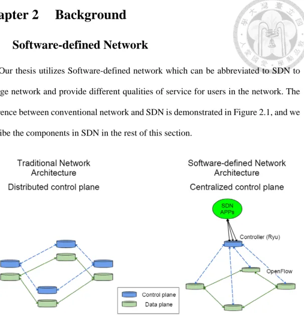
Our thesis utilizes Software-defined network which can be abbreviated to SDN to manage network and provide different qualities of service for users in the network. The difference between conventional network and SDN is demonstrated in Figure 2.1, and we describe the components in SDN in the rest of this section.
Figure 2.1: The difference between traditional network and SDN.
2.1.1 SDN Architecture
SDN is an approach to allow network administrators to manage network services through abstraction of low-level functionality. This ability is enabled with the help of decoupling the system into control plane and data plane. The control plane figures out the data path, and the data plane transfers the data according to the instructions come from the control plane.
In contrast to the conventional switches and routers, switches in SDN have no idea of how to deal with the packets by themselves. The switches in SDN called SDN switches
are controlled by a central controller. Once the switch doesn’t know how to deal with the packet, the packet will be sent to the controller. The controller will determine the data path of this packet which is the solution of how to process and transmit this packet, and the SDN switch will process the packet according to the instruction. To fulfill the tasks mentioned before, there is a need to have a protocol to boost the connections between the controller and switches. The most common protocol that enables SDN is OpenFlow which we describe in the next paragraph.
2.1.2 OpenFlow
OpenFlow is a mechanism used in SDN for the communication between control plane and data plane. This protocol was first announced in 2008 [10]. It enables switches from different vendors which have their own proprietary interfaces and scripting languages, to communicate with others using OpenFlow protocol. The inventor of this protocol considers OpenFlow as the enabler of SDN.
OpenFlow defines all of the solutions for the traffic using the concept of flow which can be statically or dynamically programmed by the SDN control software. The OpenFlow protocol requires switches to process packets according to the flow entries in their flow table. There are several fields in a flow entry, and the most important two fields are match field and instruction field which define which packet we should apply the flow entry to and what to do with the packet. If the packet doesn’t match any of the flow entry, the action is determined by the setting of table-miss entry which is often set to forward the packet to the controller. After forwarding to the controller, the controller will generate a new flow entry for this packet and adds this entry to the switch’s flow table.
In summary, the OpenFlow protocol defines the interaction between the controller and switches, but there is still a need to implement this protocol to make SDN work. Ryu
2.1.3 Ryu
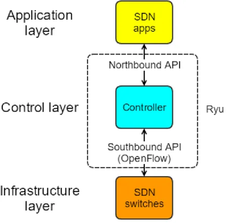
Ryu [11] is an open-source framework that integrates the implementation of southbound APIs such as OpenFlow to communicate with SDN switches and northbound APIs for the services and applications to communicate with the controller. Therefore, SDN applications can manipulate the network devices directly with the aids of northbound and southbound APIs. Furthermore, the components in the SDN organize in three layers including application, control, and infrastructure layer. The northbound APIs are used for the interactions between application layer and control layer, and the southbound APIs are used for the interactions between control layer and infrastructure layer. Figure 2.2 shows the relationship between Ryu and other components in SDN.
In the Ryu framework, a SDN application is a python script which defines the workflow of controller with the help of the Ryu library.
Figure 2.2: The illustration of the relationship between Ryu and other components.
2.1.4 Mininet
Mininet [12] is a network emulation orchestration system which enables users to construct the custom Software-defined network fast and easily. It runs virtual end-hosts, switches, links on a single Linux kernel with the help of Linux container which is a technique of lightweight virtualization. It provides many python APIs for network creation and settings, and some example codes to demonstrate how to construct sophisticated networks. Furthermore, we can configure the network elaborately, such as the bandwidth, loss rate, delay and connected port numbers of links. Because of the powerful capabilities and the convenience of Mininet, we use it to emulate our network.
2.2 Peer to peer
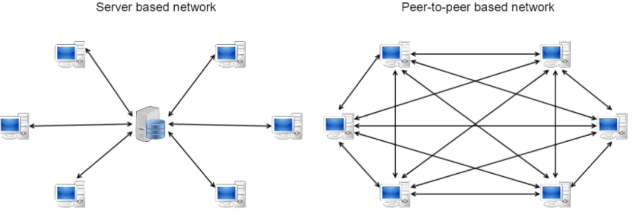
Peer to peer which can be abbreviated to P2P is a network architecture unlike client- server model and it separates the workload of server to every user in the network. Every user in P2P network is both client and server. Figure 2.3 shows the illustrations of a server based network and a P2P network. P2P network has been utilized widely in the field of file sharing, video streaming, and the applications with the requirement of high confidentiality. Our thesis focus on BitTorrent system among several file sharing systems.
Figure 2.3: The illustration of server based network and P2P network.
2.2.1 BitTorrent
BitTorrent which can be abbreviated into BT is a P2P file sharing application and a protocol developed by B. Cohen. There are many P2P applications support the BitTorrent system, and we use Deluge in our experiments. BT has become the most popular P2P file sharing system because of its efficiency in distributing large files. There are three characters in BT system: tracker, seeder and leecher. The tracker is responsible for tracking the activities, status of peers and giving the list of existing peers to new peer to contact. Next, seeders are those who have the whole file and want to share it. Finally, leechers are those who want to download the files and join the system. The files transmitted in BT system are split into several blocks which are called pieces to facilitate parallel downloading.
2.3 Incentive policy in BitTorrent
In order to increase the efficiency of transmission and the utilization of resources, an incentive policy is used in BitTorrent system which is called choking algorithm. The choking algorithm is a variant of tit-for-tat which is a strategy in game theory, and it attempts to achieve pareto efficiency which means no two counterparties can make an exchange and both benefit more from each other in economic theories. The algorithm seeking pareto efficiency is a local optimization algorithm and tends to the global optimal.
Each peer is responsible to maximize its own download speed, so they choke peers who are not willing to cooperate and unchoke peers who are willing to cooperate. Choking is a temporary refusal to upload, but it is irrelevant with download. Therefore, the users still can download files from the choked peer. In the BitTorrent system, each peer always unchokes fixed number of peers which is four in our system, so the key of choking algorithm focuses on which peer to unchoke. The decision of which peer to unchoke
depends on the download speed, and it uses the average of download speed in twenty seconds to make the measurement accurate. If the peers have finished their download, the decision of whether to unchoke this user relies on the upload rate. Each user unchokes the peers with the first four connection situations. To prevent the resources from being wasted by choking and unchoking peers frequently, the peers in BitTorrent decide which peer to unchoke every ten seconds which is also long enough for TCP to show their full capacities.
Aiming to avoid the situation that there is a current unused connection has better capacity than those being used, each BitTorrent user has an optimistic unchoked peer which means the peer can be unchoked regardless of current download speed, and the choose of optimistic unchoked peer is made every thirty seconds which is long enough for the peer to show his capacity.
In addition to above optimistic unchoked peer, a peer might be choked by all peers sometimes, and that peer might continue to get poor download speed until he was chosen as optimistic unchoked peer. There is a function called anti-snubbing that BitTorrent assumes the peer is snubbed if he doesn’t get any single piece over more than one minute, and that peer will be added as an additional optimistic unchoked peer by others to make him recover faster.
2.4 Deluge
Deluge [13] is a cross-platform BitTorrent client which is written in python and is also an open source software. Deluge uses Libtorrent [14] which is a C++ implement of the BitTorrent protocol to provide the network logic of Deluge. The architecture used in Deluge is divided into front and back end. The back end in deluge is called daemon and it can be connected by a deluge GUI console, a text console, or a web interface. We use the RPC client to connect to the daemon in our experiments.
2.5 Random Forest Classifier
Random Forest is an ensemble learning method for classification, regression, which was first proposed in 1998 [15]. It consists of several of decision trees and the decision trees in Random Forest are made by the data bootstrapped from the training data.
Bootstrap is to sample data from the original data uniformly with replacement. Therefore, the data might be chosen more than once to generate decision tree. Furthermore, the result of Random Forest classifier is the most common result among the results made by the decision trees in Random Forest classifier. Therefore, Random Forest has not only the aggregation of data but also the aggregation in model.
Chapter 3 Simulation
We describe the network topology and settings in Section 3.1. In Section 3.2 to 3.4, we show the explanations of components used in our simulation, including the deluge client, the data center, the tracker, and the controllers. We introduce the way we define the user behavior and user types at the end of this chapter.
3.1 Environment
As the Figure 3.1 shows, the network emulated by Mininet consists of three subnets, and each subnet is governed by one Ryu controller. The middle subnet is SDN network, and others are traditional networks whose topologies are deployed like a binary tree.
Furthermore, there is a NAT agent emulated by Mininet in SDN switch, and hosts access the resources outside the internal network through this agent. It is necessary to have this NAT agent, because the tracker and the data center are outside the emulated network. In addition to those, there is one host outside these three subnets to provide data in the beginning and the reason why we put that host outside the network is to make sure the traffic sent from that host controlled by the SDN network. On the other hand, the NAT agent must be placed near the SDN switch to make sure that the traffic go through the SDN network.
3.2 Deluge Client
In order to automatically control all of the hosts by ourselves, we use a lightweight Deluge RPC client on the GitHub [16] edited by user JohnDoee. It is written in python and contents with our requirement. Deluge RPC client provides libraries to interact with Deluge daemon directly.
To configure the actions of each host, we define a series of actions in the scripts. We write a program to enable each host to execute their works by reading their script and using Deluge client’s libraries to accomplish corresponding tasks. In addition, the program is set to transmit user data to data center periodically.
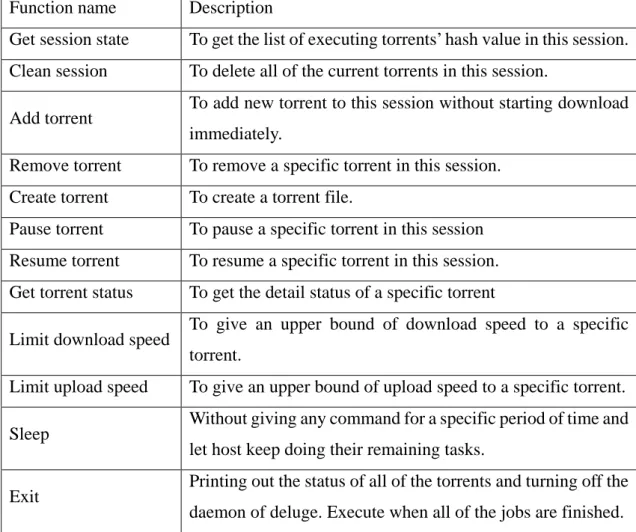
The functions in Table 3.1 are the functions that we used in our simulation.
Function name Description
Get session state To get the list of executing torrents’ hash value in this session.
Clean session To delete all of the current torrents in this session.
Add torrent To add new torrent to this session without starting download immediately.
Remove torrent To remove a specific torrent in this session.
Create torrent To create a torrent file.
Pause torrent To pause a specific torrent in this session Resume torrent To resume a specific torrent in this session.
Get torrent status To get the detail status of a specific torrent
Limit download speed To give an upper bound of download speed to a specific torrent.
Limit upload speed To give an upper bound of upload speed to a specific torrent.
Sleep Without giving any command for a specific period of time and let host keep doing their remaining tasks.
Exit Printing out the status of all of the torrents and turning off the daemon of deluge. Execute when all of the jobs are finished.
Table 3.1: The functions used in our deluge client.
When it comes to the production of user scripts, the diversity of user scripts is created by the random starting time of each torrent which are selected from first half of the overall time and the random ratios of download volume to upload volume. We explain about the ratio in session 3.6 and 3.7. The script used in our experiment looks like the following example.
Script example:
Clean_session
Add_torrent torrent_A
Limit_download_speed torrent_A 500 Limit_upload_speed torrent_A 500 Resume_torrent torrent_A
Sleep 10
Add_torrent torrent_B
Limit_download_speed torrent_B 500 Limit_upload_speed torrent_B 500 Resume_torrent torrent_B
Sleep 100
Get_torrent_status torrent_A Get_torrent_status torrent_B Exit
3.3 Tracker
Aiming to simplify our experimental environment and extract the information in the tracker, we build a tracker on our own. We use a simple BitTorrent library on the GitHub [17] edited by user JosephSalisbury which is written in python entirely and can make us
incorporate the BitTorrent protocol into our program easily. Therefore, we can deploy a tracker by using it easily.
The following are the procedure of a p2p client communicates with a tracker.
1. The client sends request using HTTP method GET.
2. The tracker decodes the request url to get information of the request such as the client’s IP address, the torrent’s hash value, and the peer id.
3. The tracker returns the list of peers’ id and IP addresses corresponding to the request torrent.
4. The client makes connections with other peers to obtain the data.
3.4 Data Center
In order to predict the type of user behavior, we gather all of the information sent from SDN switches, hosts, and the tracker to the data center via TCP connections. The data center not only saves these data but also extracts features from these raw data to classify user behavior. Furthermore, data center varies the score of hosts according to the type of user behavior and decides whether to limit or to ascend the download speed of each host depending on the score of users periodically. Data center takes advantage of OVSDB (OpenvSwitch Database) to establish queues to limit the download speed of hosts and the decision of whether to reconfigure the queues is made right after updating the score of users. Therefore, the decision is made as frequently as data center updates the score of users
3.5 Controller
In order to separate the workload and adjust controllers precisely, we use three Ryu controllers in our experiments and allocate one controller for each subset. We run the
the QoS function on the controller which governs the middle subnet which is called SDN subnet. Furthermore, we add the flows which are used to enable the p2p system on our own so as to make the flows more specific for us to manage. Instead of using the destination MAC address regardless of the Ethernet type to design the flows, we design these flows according to the source and destination IP address, and Ethernet type of the packets such as TCP, UDP and IP. On the other hand, we use the simple_switch_13.py for other two subnets without adding any flow on our own.
3.6 User Behavior
As mentioned above, every user script has a random ratio of download volume to upload volume. The clients maintain the ratio as possible as they can during executing.
More precisely, once the uploaded volume excesses the quota it can upload, the maximum upload rate will be adjusted to a very small value which can also be regarded as not allowing to upload anymore. Therefore, the host will not be capable of uploading until the quota to upload is sufficient again. The precise definition of ratio and quota are defined in the Equation 3.1.
Ratio =𝐷𝐷𝐷𝐷𝐷𝐷𝐷𝐷𝐷𝐷𝐷𝐷𝐷𝐷𝐷𝐷 𝑣𝑣𝐷𝐷𝐷𝐷𝑣𝑣𝑣𝑣𝑣𝑣 𝑈𝑈𝑈𝑈𝐷𝐷𝐷𝐷𝐷𝐷𝐷𝐷 𝑣𝑣𝐷𝐷𝐷𝐷𝑣𝑣𝑣𝑣𝑣𝑣 Upload quota = 𝐷𝐷𝐷𝐷𝐷𝐷𝐷𝐷𝐷𝐷𝐷𝐷𝐷𝐷𝐷𝐷 𝑣𝑣𝐷𝐷𝐷𝐷𝑣𝑣𝑣𝑣𝑣𝑣
𝑅𝑅𝐷𝐷𝑅𝑅𝑅𝑅𝐷𝐷
Equation 3.1: The equations of ratio and upload quota.
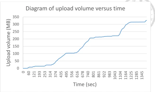
Due to the trait of retaining the ratio, the diagram of upload volume versus time might looks like Figure 3.2 which has some straight lines in the diagram if a user’s upload volume often goes beyond the quota. However, if a user’s upload volume seldom surpasses the quota, the diagram of upload volume versus time looks like Figure 3.3 which is similar to a linear line.
Figure 3.2: Example diagram of user who often violates the ratio.
Figure 3.3: Example diagram of user who almost obeys the ratio all the time.
3.7 User type
In order to find a standard which is general enough and is able to present the P2P 0
50 100 150 200 250 300 350
0 60 121 193 253 314 374 435 495 556 616 678 740 801 861 922 983 1043 1104 1164 1225 1285 1345
Uplo ad v olume (MB)
Time (sec)
Diagram of upload volume versus time
1000 200300 400500 600700 800900 1000
0 60 120 194 254 314 375 437 498 558 619 679 740 801 861 922 982 1043 1103 1164 1224 1285 1345
Uplo ad v olume (MB)
Time (sec)
Diagram of upload volume versus time
solution [18] for our application which is purposed by Manaf Zghaibeh and Kostas G.
Anagnostakis. They use clustering to divide BitTorrent users with distinctive trends into four clusters and analyze them by the ratio of upload speed to download speed. The users in the first cluster profit as much as the volume they benefit system. Therefore, the volume downloaded by them almost equals to the volume uploaded by them. Furthermore, the users in the second cluster contributed more than twice the volume they downloaded.
After that, the users in the third cluster are those who only want to download such as free riders. Therefore, volume downloaded by them exceed twice the volume uploaded by them. Finally, the users in the last cluster download less than twice the volume they uploaded, but the volume downloaded by them is still more than the volume they uploaded. In conclusion, we can summarize these attributes by the ratio of download volume to upload volume which is the download volume divided by the upload volume.
Consider the real situation in reality, we think those who download as much as they upload are brilliant users, and those who download less than twice of the volume they upload should be regarded as normal users. Therefore, we also define our classification in a similar way as following equation.
User behavior class =
⎩⎪
⎪⎪
⎨
⎪⎪
⎪⎧ 0, 𝑅𝑅𝑖𝑖 0 ≤𝐷𝐷𝐷𝐷𝐷𝐷𝐷𝐷𝐷𝐷𝐷𝐷𝐷𝐷𝐷𝐷 𝑣𝑣𝑈𝑈𝐷𝐷𝐷𝐷𝐷𝐷𝐷𝐷 < 1 1, 𝑅𝑅𝑖𝑖 1 ≤ 𝐷𝐷𝐷𝐷𝐷𝐷𝐷𝐷𝐷𝐷𝐷𝐷𝐷𝐷𝐷𝐷
𝑣𝑣𝑈𝑈𝐷𝐷𝐷𝐷𝐷𝐷𝐷𝐷 < 2 2, 𝑅𝑅𝑖𝑖 2 ≤ 𝐷𝐷𝐷𝐷𝐷𝐷𝐷𝐷𝐷𝐷𝐷𝐷𝐷𝐷𝐷𝐷𝑣𝑣𝑈𝑈𝐷𝐷𝐷𝐷𝐷𝐷𝐷𝐷 < 5 3, 𝑅𝑅𝑖𝑖 5 ≤ 𝐷𝐷𝐷𝐷𝐷𝐷𝐷𝐷𝐷𝐷𝐷𝐷𝐷𝐷𝐷𝐷𝑣𝑣𝑈𝑈𝐷𝐷𝐷𝐷𝐷𝐷𝐷𝐷 < ∞ Equation 3.2: The definition of class of user behavior.
Chapter 4 User classification and Punishment
In our experiments, the overall execution time is one thousand and four hundred seconds. The SDN switch, hosts, and the tracker send their information to the data center every three seconds and the data center classifies user behavior every two hundred seconds. The ground truth of the type of user behavior is determined by the metric mentioned in Equation 3.2. Because we simulate the whole P2P environment and define the users’ behavior by download and upload volume ratio on our own, we know how to classify the type of user behavior. But if the data of user behavior were not generated by ourselves, we won’t know how to classify user behavior. Therefore, we have to pretend that we don’t know how to classify them. However, in order to classify user behavior without knowing the real classification method, we choose machine learning as our method to achieve this goal. After being able to classify user behavior, we design a mechanism to derive the score of users and give rewards or punishments to users depending on their score. Furthermore, the rewards and punishments are presented in the form of the upper bound of download speed and they are achieved with the help of Ryu- QoS and OVSDB.
4.1 User classification
In this section we introduce the features we used for our machine learning model.
4.1.1 Extracted features
Because the raw data for our machine learning model are collected from the SDN switch, the tracker, and P2P users, we introduce each of them in the order of where they were extracted from.
34 Features come from SDN switch
more elaborate features from UDP packets.
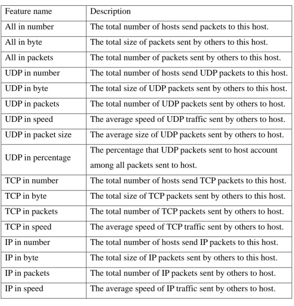
Noted that the flows using Ethernet type IP in the below apply to the traffic using IPv4 but not UDP or TCP.
Flows indicate packets sent into host:
Table 4.1: Features extracted from the flows in the direction of going into the host.
Feature name Description
All in number The total number of hosts send packets to this host.
All in byte The total size of packets sent by others to this host.
All in packets The total number of packets sent by others to this host.
UDP in number The total number of hosts send UDP packets to this host.
UDP in byte The total size of UDP packets sent by others to this host.
UDP in packets The total number of UDP packets sent by others to host.
UDP in speed The average speed of UDP traffic sent by others to host.
UDP in packet size The average size of UDP packets sent by others to host.
UDP in percentage The percentage that UDP packets sent to host account among all packets sent to host.
TCP in number The total number of hosts send TCP packets to this host.
TCP in byte The total size of TCP packets sent by others to this host.
TCP in packets The total number of TCP packets sent by others to host.
TCP in speed The average speed of TCP traffic sent by others to host.
IP in number The total number of hosts send IP packets to this host.
IP in byte The total size of IP packets sent by others to this host.
IP in packets The total number of IP packets sent by others to host.
IP in speed The average speed of IP traffic sent by others to host.
Flows indicate packets sent from the host:
Table 4.2: Features extracted from the flows in the direction of going out of the host.
Feature name Description
All out number The total number of hosts this host sends packets to.
All out byte The total size of packets sent by this host.
All out packet The total number of packets sent by this host.
UDP out number The total number of hosts this host sends UDP packets to.
UDP out byte The total size of UDP packets sent by this host.
UDP out packets The total number of UDP packets sent by this host.
UDP out speed The average speed of UDP traffic sent by this host.
UDP out packet size The average size of UDP packets sent by this host.
UDP out percentage The percentage that UDP packets sent by this host account among all packets sent by this host.
TCP out number The total number of hosts this host sends TCP packets to.
TCP out byte The total size of TCP packets sent by this host.
TCP out packets The total number of TCP packets sent by this host.
TCP out speed The average speed of TCP traffic sent by this host.
IP out number The total number of hosts this host sends IP packets to.
IP out byte The total size of IP packets sent by this host.
IP out packets The total number of IP packets sent by this host.
IP out speed The average speed of IP traffic sent by this host.
6 Features come from tracker
There are two sorts of information can be retrieved from the tracker including peer lists and the events sent from hosts. We concentrate on the data of events because they are more informative and have more benefits for us. There are three kinds of events defined in BitTorrent protocol including started, stopped, and completed. In addition, hosts send their status to the tracker without specified their event type at regular intervals.
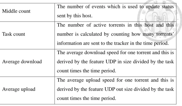
Table 4.3: Features extracted from the tracker.
Feature name Description
Started count The number of started events sent by this host.
Middle count The number of events which is used to update status sent by this host.
Task count
The number of active torrents in this host and this number is calculated by counting how many torrents’
information are sent to the tracker in the time period.
Average download
The average download speed for one torrent and this is derived by the feature UDP in size divided by the task count times the time period.
Average upload
The average upload speed for one torrent and this is derived by the feature UDP out size divided by the task count times the time period.
6 Features come from P2P users
The hosts send data which are obtained by the deluge API get_torrents_status, and they are the most accurate information of hosts. We used few of them to avoid being too dependent on the user’s data which might affect flexibility of our system.
Table 4.4: Features extracted from the hosts.
Feature name Description
Active percentage
The percentage of time that torrents are active which means torrents not pause accounts among all of the time after torrents are added.
Seeding percentage
The percentage of time that torrents are seeding accounts among all of the time after torrents are added.
Average payload download speed
The average download speed of host only considers the volume used for downloading data.
Average payload upload speed
The average upload speed of host only considers the volume used for uploading data.
Average upload speed limit
The average upload speed limit in the time period. This feature is made because the hosts maintain their download and upload ratio via restricting their upload speed.
Number of peer The maximal number of peers in the peer list in the time period.
4.2 Punishment
For the sake of being eager to make users have different user experience when they are using P2P software, we try to fulfill this target by using meter table or Ryu-QoS. As a result, OpenvSwitch doesn’t support meter table which is used to manipulate QoS with the real OpenFlow switch. Therefore, we use Ryu-QoS to achieve our goal. Next, we introduce how Ryu-QoS works with OVSDB and the configurations for the queues we used in our experiments.
4.2.1 Ryu-QoS
Ryu-QoS governs the QoS with the help of queues which are established by OVSDB, and the function of QoS are achieved by putting packets into queues. Then, queues pop the packets at the speed that we set before. In order to achieve this, the Ryu controller have to run a modified script, and there is a guide of how to modify and use this function on the official website [19]. In the official website, they modify the script from simple_switch_13.py, and we also apply this modified script to our controller to achieve QoS.
There are two flow tables in the SDN switch when running the modified script, and the flow of asking controller when switch runs into unknown traffic is set to table one.
The flows in table zero are flows that direct packets to specified queue with higher priority
priority. The action of those packets went into queues are determined by flow table one after being popped out from the queues. Therefore, we can set the flows for those packets at table one to control the action of those packets.
When it comes to the settings of queues, the queues are set at each port. The queues are set at the port which the packets leave the switch. In other words, the packets won’t be put into the queues which are set at the port that the packets enter switch. Therefore, if we want to limit the download speed of one host, we should set the limit to the queues which are set at the port that the switch connects to the host.
4.2.2 Incentive policy
As mentioned before, our machine learning model classifies the types of user behavior every two hundred seconds, and the total execution time of experiments is one thousand a four hundred seconds. Therefore, there are seven results of the type of user behavior. If we punish or reward users depending on one result, we might mistake users easily. As a result, we assign a score for each user, and the scores update after each classification. Once the score of a user exceeds the boundary we designed, the limit of download speed of that user will be increased or decreased. In addition, we think the user behavior in the first two hundred seconds might be inaccurate, because users just start downloading in that period. To avoid this problem, we ignore the first result of the type of user behavior when deriving the score of users. On the other hand, in order to decrease the throughput of users whose contribution is minor, we limit the download speed of the users who have extremely low score according to the average speed they ran in the last period.
Every user has fifty points for their score in the beginning, and the ways to adjust the score are described in Table 4.5. The limits of download speed and boundary
Table 4.5: The punishments and rewards according to the type of user behavior.
User behavior class Punishments and rewards
Class 0 + 10
Class 1 + 0
Class 2 - 5
Class 3 - 10
Table 4.6: The limits of download speed and boundary conditions.
User score Limit of download speed
Score >= 70 1.1 * Original limit of download speed Score <= 30 0.8 * Original limit of download speed
Score <= 20 0.8 * Average download speed in the last period
Chapter 5 Evaluation
5.1 Hardware and Network Settings
We construct our environment on two quad-core computers equipped with 48G and 24G RAM, and both of them are equipped with Intel I7-6700 whose processor base frequency is 3.4 GHz. The first computer runs Mininet to emulate the network and hosts, a tracker, and the program to transmit flows in SDN switch. The other one runs three Ryu controllers, the data center, and one deluge client.
The versions of Mininet and Ryu are 2.3.0 and 4.2, and the OVS (OpenvSwitch) using in Mininet has upgraded to version 2.5.0. The OpenFlow used in our environment is OpenFlow 1.3 which supports more flexible functionalities than OpenFlow 1.0.
In our setting, there is one switch in SDN network which is the middle subnet, and there are 31 switches and 32 hosts in other two subnets. The IP addresses of the subnet on the left hand side range between 10.0.0.1 to 10.0.0.32, and the IP addresses of the subnet on the right hand side range between 10.0.0.101 to 10.0.0.132.
5.2 User Settings
As mentioned in Equation 3.2, we classify user behavior into four classes, and we design our hosts with different ratios in uniform distribution of the definition of types of user behavior. Because the hosts do their best to insist the ratio of download volume to upload volume, the number of users in different user behavior type judged by each classification in the experiment are almost in uniform distribution. But the results still might be influenced by network, so the proportion of each type of user behavior might vary in reality. Every host needs to download three files in different sequence and start time, and all of these files are in size of 1GB. Table 5.1 is the list of hosts we set in
of ratio and class of users and the results of users at the end of the experiment.
Furthermore, the whole settings of original ratio and class of users and the result of users at the end of the experiment are listed in the appendix A1 The settings and results of ratio and the results in the experiment..
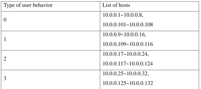
Table 5.1: The list of hosts in different types of user behavior in our experiment.
Type of user behavior List of hosts
0 10.0.0.1~10.0.0.8,
10.0.0.101~10.0.0.108
1 10.0.0.9~10.0.0.16,
10.0.0.109~10.0.0.116
2 10.0.0.17~10.0.0.24,
10.0.0.117~10.0.0.124
3 10.0.0.25~10.0.0.32,
10.0.0.125~10.0.0.132
Table 5.2: Some settings and results of users in the experiment.
User (IP) Start A (secs)
Start B (secs)
Start C (secs)
Assigned ratio
Real ratio Assigned class
Real class
10.0.0.1 41 0 425 0.884916 1.245719 0 1
10.0.0.2 462 197 0 0.039914 0.674308 0 0
10.0.0.3 96 317 0 0.371101 1.315166 0 1
10.0.0.4 399 0 8 0.48192 0.736168 0 0
10.0.0.5 409 0 99 0.677273 0.818456 0 0
10.0.0.6 0 314 128 0.114866 0.773157 0 0
10.0.0.7 191 0 367 0.339948 0.779852 0 0
10.0.0.8 0 271 78 0.719426 1.033248 0 1
10.0.0.9 85 0 324 1.821038 1.818343 1 1
10.0.0.10 334 0 32 1.830658 1.825156 1 1
10.0.0.11 342 58 0 1.460213 1.446598 1 1
10.0.0.13 0 122 297 1.262097 1.254572 1 1
10.0.0.14 40 0 293 1.795436 1.870463 1 1
10.0.0.15 0 105 239 1.800277 1.795916 1 1
10.0.0.16 374 47 0 1.550406 1.535334 1 1
10.0.0.17 0 400 105 4.4205 4.520563 2 2
10.0.0.18 0 96 358 4.809924 3.764251 2 2
10.0.0.19 252 31 0 2.079854 2.047977 2 2
10.0.0.20 0 382 162 4.155343 3.895669 2 2
10.0.0.21 135 312 0 4.28031 3.611666 2 2
10.0.0.22 0 181 408 2.92458 2.784938 2 2
10.0.0.23 0 241 34 3.366207 3.351925 2 2
10.0.0.24 106 312 0 4.766747 4.654298 2 2
10.0.0.25 34 0 365 789.8285 8.804476 3 3
10.0.0.26 192 0 398 153.9201 8.879986 3 3
10.0.0.27 212 358 0 423.3413 7.045266 3 3
10.0.0.28 350 0 4 76.7151 8.501106 3 3
10.0.0.29 0 10 252 811.758 10.74125 3 3
10.0.0.30 325 20 0 538.2712 8.527871 3 3
10.0.0.31 0 129 328 971.1503 6.38173 3 3
10.0.0.32 103 0 435 547.7919 6.940522 3 3
There are some optimization functions in deluge which are activated by default. In the general condition, if we don’t want to turn on these optimization functions, we can deactivate them by canceling the options in the GUI directly. However, we have to modify the default value of those optimization functions by ourselves in our experiments because Deluge client doesn’t provide library to adjust preference options. There are two optimization functions that we think they might influence the results of our experiments, and we turn them down. The first one is to ignore limits on the local network which will make our initial settings of hosts become useless and the second one is the local peer
discovery which might cause our environment become dissimilar to the real p2p environment.
5.3 Ryu-QoS setting
Owing to the need to give individual setting for each host and to separate connections’
bandwidth, we use 32 * (32 + 1) +1 queues to manipulate UDP packets which enable P2P system at ports that the SDN switch used to connect to other switches. Because there are 32 hosts in another subnet, 32 hosts in our subnet, and one host outside the emulated network, we need 32 * (32 + 1) queues to configure each connection between hosts according to their IP addresses. In addition to those, it needs one additional queue to let other traffic to go through.
However, if we only use one queue for each host, the limit we set to the queue will be the restriction on the total download bandwidth of torrents in the host. But it can’t be guaranteed that all of the torrents are confined by this mechanism, so we separate each pair of connections to control them more precisely.
As mentioned before, Ryu-QoS offers RESTful API for us to configure queues and flows for these queues. But the setting of queues for each port has to be set with one request, there is no function to add queues to a port one by one. Therefore, the number of queues for a port might be constrained by the loading RESTful service can afford. In order to solve this problem, we configure the setting of queues on OVSDB directly without communicating with Ryu-QoS. Although there are some errors in Ryu-QoS after we configure queues in this way, the mechanism functions normally.
5.4 User Behavior Classification
When it comes to the machine learning model, we choose Random Forest classifier
in python, and the parameters of our model are one hundred trees(estimators) and the maximum depth of decision trees is ten. The model is trained by 3840 data in our experiments.
Because we classify user behavior into four classes, we have to consider the accuracy of our results more carefully. If we only consider right or wrong, the difference between the result which is close to the right answer and the result which is far away from the right answer will be ignore. Therefore, we design a metric which also give partial points to estimate the accuracy of results in Table 5.3.
Table 5.3: The metric to estimate accuracy of results.
Result Answer
Class 0 Class 1 Class 2 Class 3
Class 0 1 0.8 0 0
Class 1 0.8 1 0.6 0
Class 2 0 0.6 1 0.8
Class 3 0 0 0.8 1
As we mentioned before, we classify the user behavior every two hundred seconds, and the score of each user is updated at the same time. On the other hand, the limits of download speed also vary simultaneously. Table 5.4 demonstrates the accuracy of our classifications and Table 5.5 shows the classifications of each class in the experiment. As shown by Table 5.5, the accuracy of class 2 and class 3 users which we concerned more are higher than others. Furthermore, the classification results in our experiment are put in the appendix A2 The results of each classification in the experiment.
Table 5.4: The accuracies and scores of our result.
Time (secs) Original accuracy Accuracy using our metric
200 0.9375 0.98125
400 0.875 0.95625
600 0.875 0.9625
800 0.84375 0.95
1000 0.78125 0.94375
1200 0.6875 0.88125
1400 0.78125 0.91875
Table 5.5: The results of each class in classifications.
Result
Class Class 0 Class 1 Class 2 Class 3 Accuracy
Class 0 66 59 0 0 58.928571
Class 1 4 67 37 4 59.821429
Class 2 0 7 83 22 74.107143
Class 3 0 1 32 79 70.535714
5.5 Punishment Results
We have shown the results of classification in the last section. The punishments and rewards for scores and the restrictions of download speed are defined in Table 4.5 and Table 4.6. We demonstrate the scores of some users in each class in our experiment in Figure 5.1 to Figure 5.4. Most of the scores of users we defined in class 0 are monotonically non-decreasing, and most of the scores of users we defined in class 3 are also monotonically non-increasing. Both of these results meet our anticipation. Although
restricted. When it comes to the results of users in class 2, we can tell the difference between them and the users in class 3 by observing the trend of scores. Most of their scores of users in class 2 are still higher than the scores of users in class 3. Next, we show part of the results of limit of download speed in our experiment in Figure 5.5 to Figure 5.8. The results of them are highly correlated with the scores of users, and we can also observe the difference between users from this view. We put all of the scores of users in our experiment in the appendix A3 The scores of users in our experiment, and all of the limits for users in the appendix A4 The limits of download speed in the experiment.
Figure 5.1: The scores of some users in class 0.
60
50
60 60 60
70 70
60 60
70
80
90
100 100
50 50 50 50 50 50 50
60 60
70
80
90 90
100
40 50 60 70 80 90 100
200 400 600 800 1000 1200 1400
Sc or e
Time (secs)
Scores of some users in class 0
10.0.0.1 10.0.0.2 10.0.0.3 10.0.0.4
Figure 5.2: The scores of some users in class 1.
Figure 5.3: The scores of some users in class 2.
50 50 50
45
40
35
30
50 50 50
45
35 35
30 50
45 45
40 40 40 40
50
45
40 40 40 40 40
25 30 35 40 45 50 55
200 400 600 800 1000 1200 1400
Sc or e
Time (secs)
Scores of some users in class 1
10.0.0.9 10.0.0.10 10.0.0.11 10.0.0.12
40 45
35 30
25 20
15
45 45
35 30
20 15
5
50 50 50
45 40
35 30
45 45
35
25 20
15 10
0 10 20 30 40 50 60
200 400 600 800 1000 1200 1400
Sc or e
Time (sec)
Scores of some users in class 2
10.0.0.17 10.0.0.18 10.0.0.19 10.0.0.20
Figure 5.4: The scores of some users in class 3.
Figure 5.5: The limits of download speed for some users in class 0.
40 40
30
20 15
10
0
45 40
30
20
10
0 0
45 40
30
20 15
10 5
45 40
30
20
10
0 0
0 10 20 30 40 50
200 400 600 800 1000 1200 1400
Sc or e
Time (secs)
Scores of some users in class 3
10.0.0.25 10.0.0.26 10.0.0.27 10.0.0.28
500 500 500 500 500 550 605
500 500 550 605 665.5 732.05 800
500 500 500 500 500 500 500
500 500 550 605 665.5 732.05 800
300 400 500 600 700 800 900
200 400 600 800 1000 1200 1400
Download speed (Bytes/s)
Time (secs)
The limits for some users in class 0
10.0.0.1 10.0.0.2 10.0.0.3 10.0.0.4
Figure 5.6: The limits of download speed for some users in class 1.
Figure 5.7: The limits of download speed for some users in class 2.
500 500 500 500 500 500
400
500 500 500 500 500 500
400
500 500 500 500 500 500 500
500 500 500 500 500 500 500
300 350 400 450 500 550
200 400 600 800 1000 1200 1400
Download speed (Bytes/s)
Time (secs)
The limits for some users in class 1
10.0.0.9 10.0.0.10 10.0.0.11 10.0.0.12
500 500 500
400
320
500 500 500
400
500 500 500 500 500 500
400
500 500 500
400
0 100 200 300 400 500 600
200 400 600 800 1000 1200 1400
Download speed (Bytes/s)
Time (secs)
The limits for some users in class 2
10.0.0.17 10.0.0.18 10.0.0.19 10.0.0.20
Figure 5.8: The limits of download speed for some users in class 3.
In order to realize the effect of limits, we show the diagram of average download speed versus time of 10.0.0.25 in Figure 5.9. The last part of the curve in Figure 5.9 goes up because the connections with users in another subnet are restricted by our mechanism, so he connects to the users in the same subnet as him. Therefore, the effect of our mechanism is limited by the number of SDN switches and the effect of our mechanism might amplifies with more SDN switches. On the other hand, we compare the average result of users in class 3 in our experiment to the average result of users in class 3 using original incentive policy in Figure 5.10. In our experiment, most of the users in class 3 are restricted by our mechanism since night hundred seconds, and the curve of our result also starts to be below the curve made by original incentive policy from then on.
500 500
400
0 100 200 300 400 500 600
200 400 600 800 1000 1200 1400
Download speed (Bytes/s)
Time (sec)
The limits for some users in class 3
10.0.0.25 10.0.0.26 10.0.0.27 10.0.0.28
Figure 5.9: The diagram of average download speed versus time of 10.0.0.25.
Figure 5.10: The comparison of average result of users in class 3.
0 10000 20000 30000 40000 50000 60000 70000 80000
200 400 600 800 1000 1200 1400
Download speed (Bytes/s)
Time (sec)
Average download speed
0 5000 10000 15000 20000 25000 30000 35000 40000
200 400 600 800 1000 1200 1400
Download speed (Bytes/s)
Time (secs)
Average download speed
Result Original
Chapter 6 Conclusion
In this thesis, we simulate different kinds of BitTorrent users via assigning different ratio of download volume to upload volume to users. We also build a tracker on our own so as to get the information of the tracker. With the help of SDN, we manipulate the network and analyze the traffic via the flows we added. Furthermore, we also get much information from switches. We can observe from the results of classification that the accuracy of our model is good enough for our experiments and the design of the score for users bears some faults when the classifications go wrong. Next, the function to give punishments and rewards which are the limits of download speed is accomplished with the aid of Ryu-QoS and OVSDB which are different from the common one used with the real OpenFlow switch. Because the decision of giving punishments or rewards to users depends on the score of users, the results of classification influence the result of experiments tremendously. Therefore, we can see the limits which are set by our mechanism for the users in the experiment are suitable for them. Furthermore, the curve of users who almost contribute nothing exactly goes down because of our punishments which is the target of this thesis.
The network environment we designed in this thesis considers the difficulty of deploying SDN in large scale which might be caused by the expensive price of OpenFlow infrastructures and the problems caused by the transformation to SDN. Furthermore, we think that the network environment can become more complicated and the way to simulate p2p user can also be more human-like.
In conclusion, we propose a mechanism that reinforces the existing incentive policy by decreasing the traffic of bad users and increasing the QoS of good users. We think it can be deployed to real world and the effect will be amplified with more SDN switches.
Bibliography
[1] RFC 1 https://tools.ietf.org/html/rfc1
[2] Official BitTorrent Specification http://www.bittorrent.org/beps/bep_0003.html [3] Cohen, B. (2003, June). Incentives build robustness in BitTorrent. In Workshop on
Economics of Peer-to-Peer systems (Vol. 6, pp. 68-72).
[4] Buragohain, C., Agrawal, D., and Suri, S. (2003). A game theoretic framework for incentives in P2P systems. arXiv preprint cs/0310039.
[5] Feng, H., Zhang, S., Liu, C., Yan, J., and Zhang, M. (2008, October). P2P incentive model on evolutionary game theory. In 2008 4th International Conference on Wireless Communications, Networking and Mobile Computing (pp. 1-4). IEEE.
[6] Wang, T. M., Lee, W. T., Wu, T. Y., Wei, H. W., and Lin, Y. S. (2012, March). New p2p sharing incentive mechanism based on social network and game theory. In Advanced Information Networking and Applications Workshops (WAINA), 2012 26th International Conference on (pp. 915-919). IEEE.
[7] Rius, J., Cores, F., and Solsona, F. (2009, October). A new credit-based incentive mechanism for p2p scheduling with user modeling. In Advances in P2P Systems, 2009. AP2PS'09. First International Conference on (pp. 85-91). IEEE.
[8] Feldman, M., and Chuang, J. (2005). Overcoming free-riding behavior in peer-to-peer systems. ACM sigecom exchanges, 5(4), 41-50.
[9] Fundation, Open Networking. "Software-defined networking: The new norm for networks." ONF White Paper (2012).
[10] McKeown, N., Anderson, T., Balakrishnan, H., Parulkar, G., Peterson, L., Rexford, J., ... and Turner, J. (2008). OpenFlow: enabling innovation in campus networks.
ACM SIGCOMM Computer Communication Review, 38(2), 69-74.
[11] Ryu https://osrg.github.io/ryu/
[12] Mininet http://mininet.org/
[13] Deluge http://deluge-torrent.org/
[14] Libtorrent http://www.libtorrent.org/
[15] Ho, T. K. (1998). The random subspace method for constructing decision forests.
IEEE transactions on pattern analysis and machine intelligence, 20(8), 832-844.
[16] Deluge RPC Client https://github.com/JohnDoee/deluge-client
[17] python-bittorent https://github.com/JosephSalisbury/python-bittorrent
[18] Zghaibeh, M., and Anagnostakis, K. G. (2007). On the impact of p2p incentive mechanisms on user behavior. NetEcon+ IBC.
[19] Ryu-QoS https://osrg.github.io/ryu-book/en/html/rest_qos.html [20] Random Forest Classifier usage in scikit-learn
http://scikit-
learn.org/stable/modules/generated/sklearn.ensemble.RandomForestClassifier.html
APPENDIX
A1 The settings and results of ratio and the results in the experiment.
User (IP) Start A (secs)
Start B (secs)
Start C (secs)
Assigned ratio
Real ratio Assigned class
Real class
10.0.0.1 41 0 425 0.884916 1.245719 0 1
10.0.0.2 462 197 0 0.039914 0.674308 0 0
10.0.0.3 96 317 0 0.371101 1.315166 0 1
10.0.0.4 399 0 8 0.48192 0.736168 0 0
10.0.0.5 409 0 99 0.677273 0.818456 0 0
10.0.0.6 0 314 128 0.114866 0.773157 0 0
10.0.0.7 191 0 367 0.339948 0.779852 0 0
10.0.0.8 0 271 78 0.719426 1.033248 0 1
10.0.0.101 0 15 390 0.65757 0.711114 0 0
10.0.0.102 227 437 0 0.185042 1.090013 0 1
10.0.0.103 340 85 0 0.153184 0.760487 0 0
10.0.0.104 286 0 118 0.679437 0.926505 0 0
10.0.0.105 0 129 311 0.532109 0.80705 0 0
10.0.0.106 370 3 0 0.09197 0.724608 0 0
10.0.0.107 0 32 450 0.867589 1.036571 0 1
10.0.0.108 264 204 0 0.83036 0.829978 0 0
10.0.0.9 85 0 324 1.821038 1.818343 1 1
10.0.0.10 334 0 32 1.830658 1.825156 1 1
10.0.0.11 342 58 0 1.460213 1.446598 1 1
10.0.0.12 0 394 225 1.888212 1.858233 1 1
10.0.0.13 0 122 297 1.262097 1.254572 1 1
10.0.0.14 40 0 293 1.795436 1.870463 1 1
10.0.0.15 0 105 239 1.800277 1.795916 1 1
10.0.0.16 374 47 0 1.550406 1.535334 1 1
10.0.0.109 303 125 0 1.84064 1.822345 1 1
10.0.0.110 0 273 119 1.191501 1.604228 1 1
10.0.0.111 0 303 59 1.89474 1.890655 1 1
10.0.0.112 39 264 0 1.925854 2.002155 1 2
10.0.0.113 0 102 327 1.446189 1.498526 1 1
10.0.0.114 0 448 190 1.261859 1.281413 1 1
10.0.0.115 226 0 280 1.547186 1.543869 1 1
10.0.0.116 0 73 463 1.994733 1.989381 1 1
10.0.0.17 0 400 105 4.4205 4.520563 2 2
10.0.0.18 0 96 358 4.809924 3.764251 2 2
10.0.0.19 252 31 0 2.079854 2.047977 2 2
10.0.0.20 0 382 162 4.155343 3.895669 2 2
10.0.0.21 135 312 0 4.28031 3.611666 2 2
10.0.0.22 0 181 408 2.92458 2.784938 2 2
10.0.0.23 0 241 34 3.366207 3.351925 2 2
10.0.0.24 106 312 0 4.766747 4.654298 2 2
10.0.0.117 443 0 77 2.758379 2.930438 2 2
10.0.0.118 0 322 78 4.765149 4.457629 2 2
10.0.0.119 0 30 334 4.474082 4.116043 2 2
10.0.0.120 334 0 133 2.735372 2.595598 2 2
10.0.0.121 447 0 0 3.588882 3.350851 2 2
10.0.0.122 3 0 238 3.236016 3.198239 2 2
10.0.0.123 147 235 0 4.221534 3.766582 2 2
10.0.0.124 46 376 0 3.627607 3.301934 2 2
10.0.0.25 34 0 365 789.8285 8.804476 3 3
10.0.0.26 192 0 398 153.9201 8.879986 3 3
10.0.0.27 212 358 0 423.3413 7.045266 3 3
10.0.0.28 350 0 4 76.7151 8.501106 3 3
10.0.0.29 0 10 252 811.758 10.74125 3 3
10.0.0.30 325 20 0 538.2712 8.527871 3 3
10.0.0.31 0 129 328 971.1503 6.38173 3 3
10.0.0.32 103 0 435 547.7919 6.940522 3 3
10.0.0.125 0 276 67 576.1131 6.972367 3 3
10.0.0.126 230 322 0 18.14696 6.031273 3 3
10.0.0.127 277 192 0 207.7989 10.28625 3 3
10.0.0.128 122 0 289 182.3024 6.311149 3 3
10.0.0.129 43 438 0 375.4619 10.16128 3 3
10.0.0.130 0 318 97 594.7106 9.332156 3 3
10.0.0.131 145 0 446 930.1203 6.979398 3 3
10.0.0.132 367 20 0 669.1685 6.266286 3 3
A2 The results of each classification in the experiment
Time
User 200 400 600 800 1000 1200 1400
10.0.0.1 0 1 0 1 1 0 1
10.0.0.2 0 0 0 0 0 0 0
10.0.0.3 1 1 1 1 1 1 1
10.0.0.4 0 0 0 0 0 1 0
10.0.0.5 1 1 1 1 1 1 1
10.0.0.6 1 1 1 1 1 1 0
10.0.0.7 0 0 0 0 0 0 0
10.0.0.8 0 0 0 0 0 0 1
10.0.0.9 1 1 1 2 2 2 2
10.0.0.10 1 1 1 2 3 1 2
10.0.0.11 1 2 1 2 1 1 1
10.0.0.12 1 2 2 1 1 1 1
10.0.0.13 1 1 0 1 0 0 1
10.0.0.14 1 1 1 3 3 1 2
10.0.0.15 1 2 1 2 2 1 2
10.0.0.16 1 1 1 1 1 1 1
10.0.0.17 3 2 3 2 2 2 2
10.0.0.18 2 2 3 2 3 2 3
10.0.0.20 2 2 3 3 2 2 2
10.0.0.21 2 3 2 2 2 2 2
10.0.0.22 2 2 2 2 2 2 2
10.0.0.23 1 2 2 2 2 2 2
10.0.0.24 2 3 2 3 2 2 1
10.0.0.25 3 3 3 3 2 2 3
10.0.0.26 2 3 3 3 3 3 3
10.0.0.27 2 3 3 3 2 2 2
10.0.0.28 2 3 3 3 3 3 3
10.0.0.29 2 3 3 3 2 3 3
10.0.0.30 3 3 3 3 3 1 3
10.0.0.31 2 3 3 3 3 2 3
10.0.0.32 2 3 3 3 3 3 2
10.0.0.101 0 0 0 1 0 1 0
10.0.0.102 0 0 1 0 0 0 1
10.0.0.103 0 0 0 0 1 0 0
10.0.0.104 1 0 0 1 0 0 0
10.0.0.105 0 1 1 0 0 1 0
10.0.0.106 1 0 1 1 0 0 1
10.0.0.107 0 1 1 0 1 0 1
10.0.0.108 1 1 1 1 0 1 0
10.0.0.109 1 1 2 2 1 3 1
10.0.0.110 2 1 0 1 1 1 1
10.0.0.111 1 1 2 2 1 1 2
10.0.0.112 1 1 2 1 1 2 2
10.0.0.113 2 2 2 1 1 1 2
10.0.0.114 2 1 2 1 1 1 1
10.0.0.115 1 1 1 2 1 2 2
10.0.0.116 1 2 1 2 2 1 2
10.0.0.117 2 1 2 2 2 2 2
10.0.0.118 3 2 2 2 2 3 2
10.0.0.119 2 3 2 3 2 3 2