可互溶流體於Hele-Shaw Cell 下界面不穩定現象─注入及拉升流場

(1)

國

立

交

通

大

學

機械工程學系

博士論文

可互溶流體於 Hele-Shaw Cell 下界面不穩定現象

─注入及拉升流場

Studies on Flow Instabilities on the Miscible

Fluid Interface in a Hele-Shaw Cell

—Injection and Lifting

研究生：

王立杰

指導教授：

陳慶耀

(2)

可互溶流體於 Hele-Shaw Cell 下界面不穩定現象

─注入及拉升流場

Studies on Flow Instabilities on the Miscible Fluid Interface in a

Hele-Shaw Cell —Injection and Liftin

g

研究生：王立杰 Student : Li-Chieh Wang 指導教授：陳慶耀 Advisor：Ching-Yao, Chen

國立交通大學機械工程學系

博士論文

A Thesis

Submitted to Institute of Mechanical Engineering College of Engineering

National Chiao Tung University in partial Fulfillment of the Requirements

for the Degree of Doctor of Philosophy

in

Mechanical Engineering

June 2014

Hsinchu, Taiwan, Republic of China

(3)

中文摘要

黏滯度指狀物是指於平行薄板或多孔性材料間，以低黏滯度流體驅動高黏度流體時，兩流體間介面形成代表流場不穩定的指狀物型態，在多種工業製程中，多相流流場界面的不穩定性，嚴重影響產品品質及生產效率，常見案例為原油開採時以水性溶劑為驅動流體注入多孔性岩層推動更為黏稠原油時，卻因指狀物型態出現，而使水性溶劑穿透原油，降低開採效率。另平行薄板間高度改變形成的徑向拉升流場，也因可運用於黏著與潤滑分析，成為另一重要研究議題，本論文中運用高精確模擬(highly accurate simulation)之數值方法，分別以一致形(monotonic)與非一致形(nonmonotonic)黏滯度剖面之可互溶流體，探討徑向注入微小間隙的兩平行板間(即 Hele-Shaw Cell)與間隙隨時間增大之Hele-Shaw Cell 徑向流場之界面演變，論文內容包含兩大部分：第一部份於注入流場進行大量系統化的數值模擬，針對不同對流／擴散比(Peclet 值)與黏滯度剖面參數討論，首先除以過去學者慣用之指數型(下凹曲線) 一致形黏滯度剖面進行研究外，另外定義線性及反指數型(上凸曲線)一致性黏滯度剖面與非一致形黏滯度剖面進行比較，結果顯示黏滯度對比固定時，各種黏滯度剖面對注入流場之穩定性無顯著影響，但如非一致性黏滯度剖面與上凸黏滯度剖面交錯，將激化流體介面間的不穩定性。另經由系統化改變非一致形黏滯度分布各參數值，觀察其對界面指狀化圖形之影響，除觀察到多種有趣之介面型態，諸如產生於一致形黏滯度分布所無法觀察到的成對雙渦旋流場及逆指狀物結構等現象，最後對非一致性黏滯度剖面各參數對整體

(4)

第二部分首先探討不同拉升函數與初始擾動對流場穩定性之影響，相對於定量注入可互溶流體於徑向Hele-Shaw Cell 流場會產生指狀物尾端開叉與分枝等多變流場現象，平行板間隙隨時間成指數化關係變化的拉升流場形成更錯綜複雜的流場現象，近期研究指出經由調整平板間隙與時間函數關係可控制流場指狀物的形態，本研究除得到指數拉升方式可較線性拉升方式獲得更不穩定之流場，亦歸納出高Péclet 值與高黏滯度對比會增加指狀物長度，另對初始條件與擾動設定對流場穩定度影響於指數函數拉升時影響較大，線性函數拉升則幾乎沒有影響。進而討論不同黏滯度剖面之可互溶流體於指數拉升流場之界面型態，影響情況較注入流場顯著。接著採與第一部份相同作法，探討不同黏滯度剖面之可互溶流體於拉升流場之影響，發現黏滯度剖面對流場穩定性影響程度於拉升流場較注入流場大，且不穩定性均遵循下凹曲線>直線>上凸曲線順序，最後對非一致性黏滯度剖面各參數對拉升流場穩定性影響進行討論。

(5)

Abstract

Viscous fingering is an interfacial fluid flow instability that occurs when less viscous fluid displaces another more viscous one in a Hele-Shaw cell or porous media, leading to the formation of finger-like pattern at the interface of both fluids. The interfacial evolution of multiphase flows will severely impact on the quality of production and efficiency in a variety of practical application of industrial process. Most frequent example of this instability is that of oil recovery for which viscous fingering takes place when an aqueous solution displaces more viscous oil in underground reservoirs, leading to the formation of nontrivial fingerlike structure and reduce the efficiency of the displacement process. Another particularly interesting variation of the classic radial flow is the investigation of fingering instabilities in Hele-Shaw cells presenting variable gap spacing. This is also a very important issue in many industrial areas including adhesion, lubrication, and colloidal hydrodynamics. In this dissertation, we carried out the highly accurate simulation to investigate the interfacial evolution in two scenarios－radial injection-driven miscible flow and lifting radial Hele-Shaw flow, both with the monotonic and nonmonotonic viscosity profile. So, the thesis consists of two parts:

Part 1 focus on radial injection-driven miscible flow in a Hele-Shaw cell and covers three major topics. To begin with, we perform numerical experiments in a wide range to study the dispersion relation on both the Péclet number and the parameters of the viscosity profile. A monotonic viscosity-concentration relation of exponential type (concave) by other scholars is assumed, and a linear and reverse (convex) monotonic viscosity profiles and nonmonotonic one are also discussed. Results of this study

(6)

viscosity profile lead to a more stable flow than that of monotonic one, and there are no significant differences in different viscosity profiles. However, if the nonmonotonic viscosity profile crosses the convex monotonic viscosity profile, the nonmonotonic feature enhances the prominence of interfacial instability. Then, a great variety of morphological behaviors is systematically introduced. In general, the nonmonotonic feature enhances the prominence of interfacial instability. Formation of dual vortex pairs and “reverse fingering”, where the fingers spread farther in the backward than in the forward direction are observed, which are not present in monotonic viscosity profile. Finally, we have carried out a parameter study to understand the effects of nonmonotonicity on the stability of the injection flow.

In part 2, discussions start with the investigation of the influence of lifting scenario and the perturbation set. Contrast to the injection-driven miscible flow in radial Hele-Shaw cells which leads to the formation of morphing flow phenomenon of finger tip-splitting and side-branch events are plentiful if the injection rate is constant with time. More complicated flow are present for time-dependent gap flow which results in different kinds of patterns, and leads to intricate morphologies if the cell’s gap width grows exponentially with time. Recent studies show that the growing of intricate patterns due to lifting can be controlled by properly adjusting the time-dependent gap width. Moreover, we found the exponential lifting case will cause the flow more unstable than the variant lifting situation. We also deduce higher Péclet number and viscous contrast (A in monotonic viscosity profile and μm in nonmonotonic one) demonstrate more vigorous

fingering. The sensitivity of the system to changes in the initial conditions and perturbation set is also discussed. Next, the effects of four viscosity profiles as stated in part 1 have been investigated. Unlike injection flow, the stability of three monotonic viscosity profiles are always in the series of

(7)

concave, linear and convex. However, as injection flow, if the nonmonotonic viscosity profile crosses the convex curve will enhances the prominence of interfacial instability. Finally, we have carried out a parameter study to understand the effects of nonmonotonicity viscosity profile on the stability of the lifting flow.

(8)

誌

謝

由衷地感謝陳慶耀教授，在原指導教授楊文美老師退休之後，願意接受一個對數值計算及流場不穩定性完全不了解的學生，讓昔為航空背景的我能夠進入此領域進行研究，且常因任務需求，無法常與您 meeting 的情況下，只能剝奪您休息時間，在新竹至台中的路途上盡量挖掘您學術及人生的寶庫，獲得您無私的分享，在此研究上能夠有些許的發現，全因為您細心指導。日後研究的範圍還很寬廣，我會將您的指導盡情揮灑出屬於我的天空。感謝大學時期曾教過我的曾培元教授及宋齊有教授，以及許立傑教授、吳宗信教授及陳彥升研究員能在百忙之中遠道而來，蒞臨指導我的學位口試，不吝給予寶貴意見，使我了解論文撰擬上的疏漏，學習到更多陳述解決問題及表達結果的技巧，謝謝各位老師的指導；也感謝曾經與我一同在實驗室共同打拼的學弟妹琦雯、裕盛及彥宏等，沒有你們的陪伴與協助還真不知如何完成這段路。就學期間涵蓋職場兩個階段，感謝空軍測評戰研中心國正、中樑、洪安及文琳主任讓我實現飛行的夢想以及求學的支持，及兄弟們的情義相挺，亦要感謝國家中山科學研究院航空研究所准予以公餘進修方式攻讀博士學位。一路走來兼顧工作與求學兩方面的負荷，父母及愛妻秀梅對家庭的照顧，使我可以無後顧之憂地全力以赴，彭老醫師精湛的醫術也使我精神及體能始終可以維持最佳狀況，芃允和心佑兩位天真活潑又可愛的女兒也總是讓我疲憊時重新燃起動力，讓我完成我的夢想。僅將本文獻給每一位曾在人生路上伴我成長的家人、師長、兄弟及朋友們，感謝你們。

(9)

List of Figures

Figure 1: Schematic illustration of a perturbation of the interface between two fluids in Hele-Shaw cell, the injecting flow1 pushes the

displaced flow2. ... 25 Figure 2: A physical interpretation of the stability criteria. ... 25

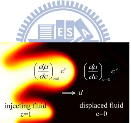
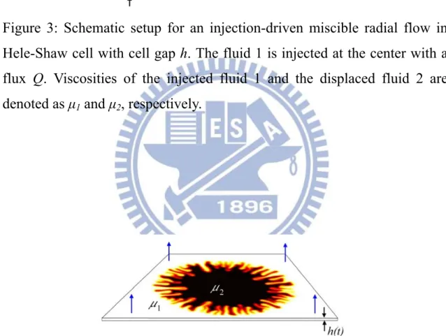
Figure 3: Schematic setup for an injection-driven miscible radial flow in Hele-Shaw cell with cell gap h. The fluid 1 is injected at the center with a flux Q. Viscosities of the injected fluid 1 and the displaced fluid 2 are denoted as μ1 and μ2, respectively. ... 26

Figure 4: Schematic setup of the time-dependent gap radial Hele-Shaw flow with miscible fluids. The upper plate of the cell is lifted, so that the gap of the cell is variable. The inner fluid is more viscous (μ2 > μ1). ... 26

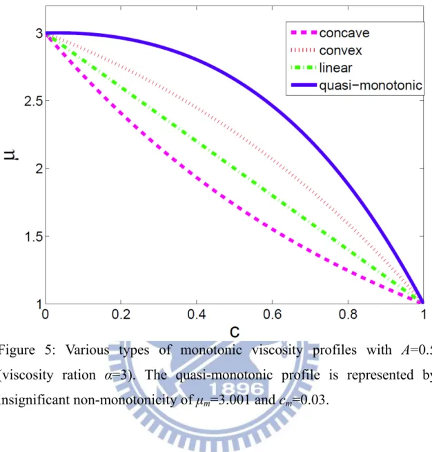
Figure 5: Various types of monotonic viscosity profiles with A=0.5

(viscosity ration α=3). The quasi-monotonic profile is represented by insignificant non-monotonicity of μm=3.001 and cm=0.03. .... 37

Figure 6: Concentration images with Pe=800 at t=0.30 for various types of viscosity profiles shown in Fig. 5, (a) concave; (b) linear; (c) convex and (d) quasi-monotonic. In the present unstable

conditions, i.e. μ1 > μ2, fingering instabilities are observed for all the profiles. The overall patterns show great similarities, which indicate insignificant influences of the local correlations between fluid concentration and the viscosity. ... 38

Figure 7: Evolutions of the interfacial lengths, which can be used as a global quantitative measurement of the prominence of fingering,

(12)

length under the condition set as Fig. 5. The global characteristics of interfacial lengths show no significant variations. Nevertheless, a general trend is observed, in which a more convex profile leads to a more unstable interface at the early time, and turns more stable at a later stage. ... 39

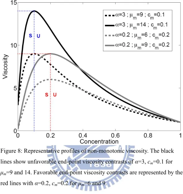
Figure 8: Representative profiles of non-monotonic viscosity. The black lines show unfavorable end-point viscosity contrasts of α=3,

cm=0.1 for μm=9 and 14. Favorable end-point viscosity contrasts

are represented by the red lines with α=0.2, cm=0.2 for μm=6 and 9.

... 40

Figure 9: Concentration images for the case of unfavorable viscosity profile (α=2, top row), and favorable viscosity profile (α=0.5, bottom row). These simulation used for different Péclet number with parameters set for μm=4 and cm=0.2 at t=0.35. ... 41

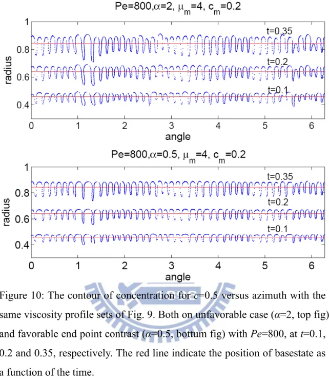
Figure 10: The contour of concentration for c=0.5 versus azimuth with the same viscosity profile sets of Fig. 9. Both on unfavorable case (α=2, top fig) and favorable end point contrast (α=0.5, bottum fig) with Pe=800, at t=0.1, 0.2 and 0.35, respectively. The red line indicate the position of basestate as a function of the time. ... 42

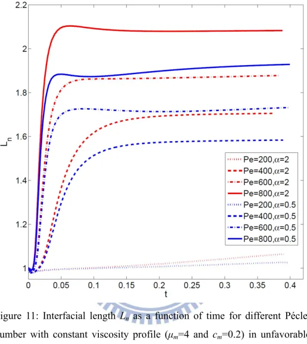
Figure 11: Interfacial length Ln as a function of time for different Péclet

number with constant viscosity profile (μm=4 and cm=0.2) in

unfavorable and favorable viscosity profile. In the inset the number label the Péclet number and end-point viscosity contrast. An interesting phenomena damping effect can be observed in

Pe=800 and α=0.5 set and will be discussed later. ... 43

Figure 12: Concentration images for the non-monotonic viscosity profiles shown in Fig. 8 with Pe=400. Unfavorable viscosity contrast of

(13)

α=3 and cm=0.1 for μm=9 (a) and μm=14 (b). Favorable viscosity

contrast of α=0.2 and cm=0.2 for μm=6 (c) and 9 (d). The

non-monotonic viscosity profile enhances fingering instability significantly. Even an original stable interface in a monotonic profile appears significantly fingering if the viscosity profile is non-monotonic, i.e. α < 1 shown in (c) and (d). In addition, the prominences of fingering are enhanced by degree of the

monotony, i.e. higher μm. ... 44

Figure 13: Correspondent images of vorticity for the cases shown in Fig. 8. Besides the well-understood vorticity pairs inside the individual fingers, additional pairs of detached vorticity caps right beyond the fingertips are generated due to the non-monotony of

viscosity profile. ... 45

Figure 14: Evolutions of the normalized interfacial lengths for the four cases shown in Fig. 8. After a short period of time with

significant growths, the interfacial lengths appear to level off. In line with the common expectations, a more unfavorable

end-point viscosity contrast, such as α=3, results in a more prominent fingering instability. Also confirmed is that significance of the viscosity non-monotony leads to a more unstable interface, e.g. μm=9. ... 46

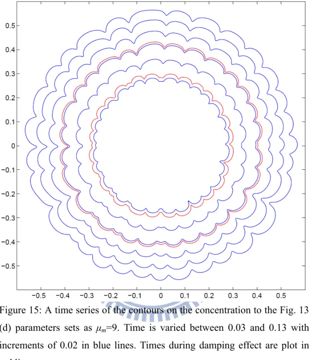
Figure 15: A time series of the contours on the concentration to the Fig. 13 (d) parameters sets as μm=9. Time is varied between 0.03 and

0.13 with increments of 0.02 in blue lines. Times during

damping effect are plot in red lines. ... 47

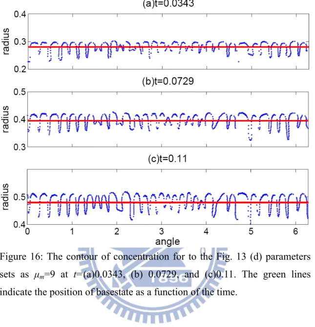
Figure 16: The contour of concentration for to the Fig. 13 (d) parameters sets as μ =9 at t=(a)0.0343, (b) 0.0729, and (c)0.11. The green

(14)

... 48

Figure 17: Representative profiles of non-monotonic viscosity for the cases with unfavorable and favorable end-point contrasts of α=3 and 0.7, respectively. The local maximum viscosity contrast is μm=4,

whose position is at cm=0.1, 0.3, and 0.5. ... 49

Figure 18: Parameter for the end-point derivatives of the viscosity profile,

Λ as a function of the maximum of the viscosity profile, cm, both

for the unfavorable and favorable end-point viscosity contrast in Fig. 17. ... 50

Figure 19: Evolutions of the normalized interfacial lengths for Pe=400 with the six viscosity profiles shown in Fig. 17. The most unstable interface at a later time stage is always triggered by a smallest

cm=0.1, whose viscosity profile appears more concave, for both

unfavorable and favorable end-point conditions. The trend

agrees well with the findings presented in Fig. 18. ... 51

Figure 20: Concentration images for the non-monotonic viscosity profiles shown in Fig. 17 with Pe=400 and μm=4 at t=0.30. Unfavorable

viscosity contrast of α=3 and cm=0.1, 0.3, and 0.5. Favorable

viscosity contrast of α=0.2 and cm=0.1, 0.3, and 0.5. The lower cm enhances fingering instability significantly. Even an original

unstable interface in higher cm appears significantly more

unstable either favorable or unfavorable shown in Fig. 19. ... 52

Figure 21: Concentration images (top row) and vorticity images (bottom row) for viscosity profile set with μm=13 and cm=0.1 for (a) Pe=400 and α=2. (b) Pe=200 and α=9. (c) Pe=400 and α=9 at t=0.30. The outer fluid is more viscous (μ2 >μ1). ... 53

Figure 22: Evolutions of the normalized interfacial lengths for Fig. 21. ... 54

(15)

and α=0.2, 0.5, and 1. ... 55

Figure 24: Concentration images (top row) and vorticity images (bottom row) for Pe=400, μm=4, cm=0.1, α=0.2, 0.5, and 1 at t=0.30. The

inner fluid is more viscous (μ1 > μ2) and the green lines in

vorticity images indicate the position of μm. ... 55

Figure 25: Time evolution of the interfacial length with μm=4, cm=0.1, α=0.2, 0.5, and 1 for Pe=400. In the inset the detail viscosity

profiles for the three parameters sets. No significant main effect for favorable end-point contrast was found. ... 56

Figure 26: Concentration images for the dimensionless gap distances

h/h0=2, 3, and 4, for the cases of exponential lifting (top row), and variant lifting (bottom row) to the parameter set as Pe=3000,

A=0.925. The domain of x and y axis are -0.8 to 0.8. ... 67

Figure 27: Concentration images for Pe=2000 (first column), 3000 (second column), 4000(third column), and A=0.762 (top row), 0.905 (mid row), 0.925 (bottom row) at dimensionless gap distances

h/h0=4, for the cases of exponential lifting. The domain of x and

y axis are -0.5 to 0.5. ... 68

Figure 28: Interfacial lengths Ls as a function of the dimensionless gap

distance h/h0 for the exponential lifting case. These simulations used the same physical parameters as in Fig. 27. In the inset the numbers label the distinct Pe and A sets. ... 69

Figure 29: A dimensionless gap distances h/h0 series of the contours on the

concentration to the parameters sets as Pe=3000, A=0.925 for the exponential lifting case. For the dimensionless gap distance

h/h0= (a) 1.5, (b) 2, (c) 2.5, and (d) 4. ... 70 Figure 30: A dimensionless gap distances h/h series of the contours on the

(16)

the variant lifting situation. For the dimensionless gap distance

h/h0= (a) 1.5, (b) 2, (c) 2.5, and (d) 4. ... 70 Figure 31: Concentration images for the dimensionless gap distance h/h0=4

for the cases of exponential lifting (top row), and variant lifting (bottom row). These simulations used the same physical

parameters as in Fig. 26, but utilized two distinct set of initial random conditions: perturbation set 2 (first column), and

perturbation set 3 (second column). ... 71

Figure 32: Interfacial length Ls as a function of the dimensionless gap

distance h/h0 for the exponential lifting (EL)case, and three different sets of initial perturbations (solid curves).The dashed curves represent similar sets of data for the variant lifting (VL) situation. In the inset the numbers label the distinct perturbation sets. ... 72

Figure 33: Concentration images for the dimensionless gap distance h/h0=2, 3, and 4 for the cases of exponential lifting. These simulations used the same physical parameters as in Fig. 29, but utilized two distinct set of initial random conditions: amplitude=0.05 (top row), and amplitude=0.1 (bottom row). ... 73

Figure 34: Interfacial lengths Ls as a function of the dimensionless gap

distance h/h0 for the exponential lifting case. These simulations used the same physical parameters as in Fig. 27. In the inset the numbers label the amplitude sets. ... 74

Figure 35: Four kinds of viscosity profiles with A=0.925 (α=25.67). The parameters set of the Quasi-monotonic viscosity profile is

cm=0.1 and μm=25.77. ... 75

Figure 36: Concentration images for the dimensionless gap distance h/h0=2, 3, and 4, for the cases in Fig. 35 with Pe=2000 and A=0.925 for

(17)

(a) Concave (b) Linear (c) Convex (d) Quasi-monotonic. The inner fluid is more viscous (μ2 >μ1). ... 76

Figure 37: Interfacial length Ls as a function of the dimensionless gap

distance h/h0 for the exponential lifting case and four kinds of different viscosity profiles for Fig. 35 with Pe=2000. In the inset the numbers label the distinct viscosity profiles. ... 77

Figure 38: Five kinds of viscosity profiles with A=0.848 (μm=eA =12.18).

The parameters set of the nonmonotonic viscosity profile is

cm=0.1 and α=10. ... 78

distance h/h0 for the exponential lifting case and five viscosity

profiles in Fig. 38 with Pe=4000. In the inset the numbers label the distinct viscosity profiles. ... 79

Figure 40: Concentration images for the dimensionless gap distance h/h0=4 with Pe=4000, for the viscosity profile depicted in Fig. 38 for (a) Concave (b) Linear (c) Convex (d) Nonmonotonic, α=10. The inner fluid is more viscous (μ2 >μ1). ... 80 Figure 41: Concentration images of parameters set α=3 and cm=0.1 with

Pe=3000 for the exponential lifting case (a) μm=8, (b) μm=16, (c) μm=24 and (d) μm=32 for the dimensionless gap distance h/h0=4, ... 81

distance h/h0 for the four cases shown in Fig. 41. In the inset the numbers label the distinct maximum viscosity μm. ... 82

Figure 43: Time evolution of the interfacial length Ls for two monotonic

viscosity profiles with α=20.08 and 16.44 and four

(18)

for the seven parameters sets. ... 83

Figure 44: Concentration images of parameters set μm=16.44 and cm=0.1

with Pe=3000 for the exponential lifting case (a) α=3, (b) α=9, (c) α=12 and (d) α=15 for the dimensionless gap distance h/h0=4. Despite the finger lengths of different cases are very close; the morphology in each set is quite similar. ... 84

Figure 45: Correspondent images of vorticity for the cases shown in Figure 43 for the dimensionless gap distance h/h0=4, (a) α=3; (b) α=9; (c) α=12 and (d) α=15 for Pe=3000. Unlike the inner fingers in injection flow, it may become disappear, as the difference

between α and μm decrease. ... 85

Figure 46: Representative profiles of non-monotonic viscosity profiles show end-point viscosity contrasts with α=3, μm=24 for cm=0.1,

0.3, 0.5 and 0.7. ... 86

Figure 47: Concentration images for the dimensionless gap distance h/h0=4 with the non-monotonic viscosity profiles shown in Fig. 46 with

Pe=2000 for series of (a) cm=0.1, (b) cm=0.3, (c) cm=0.5 and (d) cm=0.7. ... 87

Figure 48: Time evolution of the interfacial length with viscosity profile

α=3, μm=24 with Pe=2000 for cm=0.1, 0.3, 0.5 and 0.7. ... 88

Figure 49: Concentration images for the dimensionless gap distance h/h0=4 for the favorable end-point contrast cases of α=0.25 (top row), and the unfavorable end-point contrast cases of α=4. Utilized two distinct set of the location of the maximum viscosity:

cm=0.1 (first column), and cm=0.9 (second column).Other

(19)

Nomenclature

Roman Symbols

a lifting ratio

A Atwood number

b parameter of compact finite-difference

c concentration of the injecting fluid

h gap thickness

k permeability

L interfacial length

M mobility

N the number of grid point

Pe Péclet number p pressure Q injection rate R mobility ratio r radius t time u velocity vector

V volume of the fluid

v velocity vector

x, y spatial direction

Greek Symbols

(20)

γ control parameter

δ a control parameter with an inverse dimension of time.

η parameter of Runge-Kutta

μ viscosity

ν parameter of Runge-Kutta

ξ parameter of compact finite-difference



stream function Λ stability criteria ρ density σ core size Subscripts B base state c critical value

d axisymmetric divergent radial

exp exponential

f divergence free component

g grid number

i initial

linear linear viscosity profile

m maximum

mono monotonic viscosity profile

n normalized

non nonmonotonic viscosity profile

pot potential part

r rotational part

v variant dimensional lifting situation

(21)

0 initial condition

1 injection in injection flow / outer flow in lifting flow

(22)

Chapter 1 Introduction

1.1 Literatures Review

Viscous fingering (VF) is a hydrodynamic instability occurring where a higher viscous fluid is displaced by a less viscous one in porous media. It can be observed the different viscous fingering instabilities in the interface between the two fluids, and can be explained by Saffman-Tayler instability. In most applications, viscous fingering instabilities are undesirable as the displacing fluid fingers through and by pass the displaced one, reduces the efficiency of this injection. Over the years viscous fingering problem has been extensively studied both experimentally and theoretically. The related studied can be classified into two categories depending on whether the viscosity profiles are monotonic or nonmonotonic. For convenience, Tan and Homsy [1] defined a particular case in which viscosity varies exponentially with the concentration of injection fluid, as well as monotonic viscosity profiles. They also used Fourier spectral method and found as time progresses, the nonlinear behavior of fingers cause a few dominant fingers spread and shield [2]. However, some driving fluid used to petroleum secondary recovery techniques such as a mixture of alcohols and water need not to be monotonic. Manickam and Homsy [3] defined a nonmonotonic viscosity profile for the viscosity concentration data of alcohols to approximate nature fluid behavior. They have carried out a parameter study to understand the effects of nonmonotonicity on the stability of the flow. Other last strategies aim to analysis viscous fingering by non-Newtonian fluid interfaces [4].

Researchers studies have focused on simpler geometries, such as two fluids in the narrow gap between closely-spaced parallel plates of a Hele-Shaw cell, include rectilinear and radial flow, as well as quarter

(23)

five-spot configuration. Many theoretical and experimental studies have been performed in both geometrics. Tan and Homsy [1] used the quasi-steady-state approximation (QSSA) for a radial source flow in porous media with monotonic viscosity profiles. They found that the unfavorable viscosity gradient results the fluid more unstable in radial source flow. They also did a critical Péclet number Pec calculation, above which

displacement becomes unstable, and vice versa. Chen and Meiburg [5, 6] focused on miscible quarter five-spot configuration and radial flows in homogeneous and heterogeneous environment with monotonic viscosity profiles, and described in detail as a function of the mobility ratio R and the Péclet number Pe. Chen et al. [6-9] also investigate the stability of time-dependent gap Hele-Shaw cell which is significant to adhesion related problem. In addition, the results by Manickam and Homsy [10] used Hartley transform based spectral method for rectilinear flow with nonmonotonic viscosity profiles show a new phenomenon of “reverse” fingering and understand the effects of nonmonotonicity on the stabilization of the flow. Ruith and Meiburg [11] added the effect of gravity force in miscible displacement and investigate the influence of the Péclet number, the viscosity and density contrasts, and the aspect ratio on the dynamic evolution of the displacement. An up-to-date report write by Jha et

al. [12] take viscosity contrast into account to affects fluid mixing. Recent

extend the studies of the miscible flow in a rotating cell [13-17] demonstrate fingering morphologies unlike in injection and lifting flow [18].

The main difference between the radial and the rectilinear displacement is that for the rectilinear flow, the base state velocity is a constant, while for the radial displacement, the velocity decreases spatially 1/r. Nonlinear simulations of quarter five-spot configuration displacements have been

(24)

radial source flows. Pankiewitz and Meiburg [19] extend this analysis to numerical simulation of quarter five-spot configuration with nonmonotonic viscosity profiles, which have done a deliberative parameter study, and derive that either favorable or unfavorable end point contrast will cause the flow unstable only that the Péclet number is sufficiently high. They also find there exist two concentric rings of vortex region and touch each other exactly at the location of the viscosity maximum. Shariati and Yortsos [20] explained the overall effect any two adjacent counter-rotating vortices may further stabilize or destabilize the flow. As point out earlier, some late researchers study the viscous fingering by chemical means. Chemical reaction may change the density, surface tension or viscosity of the fluid. Hejanctuzi et al. [21] used linear stability analysis for a reaction-diffusion-convection problem and found the effects of chemical reaction on the stability of the flow are like nonmonotonicity.

To date, most of the previous studies (e.g. Tan and Homsy [2]; Chen and Meiburg [5]) on monotonic viscosity profile consider flow on the relation to concentration and viscosity are an exponential function. There is a noticeable absence of research projects dealing with different types of monotonic viscosity profiles. Due to the practical and academic relevance of the injecting problem, it is of interest to study and understand the emerging interfacial under many different viscosity profiles. Additionally, the effect of nonmonotonic viscosity profile on the stabilization of miscible displacement has been considered in a limited number of studies. Chouke [22] and Tan and Homsy [23] obtained stability criteria Λ can be interpreted through the slopes in injection and displaced fluid sides. They employed QSSA to analyze the stability characteristics. Loggia et al. [24] make an exhaustive study of the parameter and explain the key for of longitudinal dispersion in making conditionally unstable an initially stable profile as sufficient time. Nevertheless, Manickam and Homsy [3] used the

(25)

QSSA and suggested the equation fails to hold at large times when the base state has diffused out. Later Kim and Choi [25] tackled the problem of without QSSA and believed the system is unconditionally stable for long-wave disturbance regardless of viscosity profile.

Miscible displacements with nonmonotonic viscosity profiles are characterized by negligible surface tension, so that the interplay of by the Péclet number and the parameters of the viscosity profile dictate the pattern formation behavior. Although researchers agreed the viscosity profiles effects the stability of fluid. Not only little research has been done on the final state of the nonmonotonic viscosity profile variation system, but has never seen discussing different monotonic viscosity profile stability of the flow field. We are therefore interested in developing a fundamental understanding of miscible radial flow with monotonic and nonmonotonic viscosity profile.

Much of the research of the traditional Saffman-Taylor problem has examined the flow in flat, motionless, constant-gap spacing Hele-Shaw cells, in which the fluids are relatively simple. Somewhat simpler radial and rectangular geometry situation have been examined, where the upper plate is lifted uniformly, i.e., the plates remain parallel to each other during the lifting process. It is the so-called lifting radial Hele-Shaw flow and result Saffman-Taylor situation in the formation of complex structures.

A particularly interesting variation of the classic radial flow is the investigation of fingering instabilities in Hele-Shaw cells presenting variable gap spacing. The study of compliant adhesive layers is highly interdisciplinary involves a great variety of areas range from interfacial science and rheology to pattern formation. It is worth noting that is not only intrinsically interesting, but also of significant importance to related problems. In such types of problems, to get the bond strength of adhesives

(26)

by a thin adhesive film can be quite successfully evaluated through a Hele-Shaw approach (Darcy’s law formulation). In other industrial areas including lubrication, fracture mechanics, chemistry, biology [26], wetting dynamics, colloidal hydrodynamics [27] and oil recovery[28], lifting radial Hele-Shaw flow plays very important role.

Unlike the traditional Hele-Shaw cells of a constant gap, in such a lifting version the upper plate of the cell is moved upwards uniformly at a lifting velocity, i.e., the plates remain parallel to each other during the lifting process, while the lower plate of the cell is held fixed. The morphology of the emerging structures is characterized by the competition among inward moving fingers. To create complex viscous finger in lifting radial Hele-Shaw flow [19, 20, 22, and 29] the more viscous fluid is placed at the center of a Hele-Shaw cell, surrounded by a less viscous fluid, and the upper cell plate is moved upwards. The pressure gradient within the more viscous fluid is due to the lifting of the upper plate, the fluid-fluid interface moves inwards allowing the penetration of multiple fingers of the outer. Interesting variation of the radial Saffman-Taylor problems Hele-Shaw cells with variable gap spacing are presented which are different to with a constant gap and need to be investigated.

As the lifting radial Hele-Shaw flow where the upper plate is lifted just by one edge, making the gap both time and space dependent, where so that the gap is a function of time, but not of space. This defines the so-called

time-dependent gap Hele-Shaw cell. Shelley et al. [29] have shown the

Saffman-Taylor instability for stretch flow in rectangular geometry Hele-Shaw cells is valid both with and without surface tension, where the pressure gradient within the fluid is due to the lifting of the upper plate at a specified rate. Different kinds of pattern arise in the lifting Hele-Shaw flow where the cell’s gap varies with time. Ben-Jacob et al. [30] investigated the stability of lifting Hele-Shaw cell with rectangular geometry by experiment

(27)

obtain at low lifting rate finger formed, while the lifting velocity is increased, fingers become dendrites; and the spacing of the dendrites decreases as the lifting velocity is increased. Zhang et al. [31] performed a linear stability analysis of the issue and derived the basic equations of the directional solidification problem. Linder et al. [32] studied fingering patterns and lifting forces of a thin layer of Newtonian liquid in both numerical simulations and experiments. They have found the number of fingers is sole determined by the surface tension and the extent of fingers growth depends not only on control parameter but also on initial conditions.

A somewhat simpler radial geometry situation has been extensively studied, both experimentally and theoretically. Miranda and Oliveira [33] replaced the thin film with conventional adhesive material to a high viscosity ferrofluid between two narrowly spaced parallel flat plates a subjected to an external magnetic field. The work by Dias and Miranda [34] showed an example that finger competition is restrained as the gap width scale with time with exponent -2/7 by linear stability analysis. For this particular situation, it has been shown that finger competition is restrained leading to a more ordered array of fingers. Chen et al. [9] studied have noted that time-dependent gap miscible flow in lifting Hele-Shaw cells leads to intricate morphologies if the cell’s gap width grows exponentially with time can create more vigorous fingering process.

1.2 Objective and Organization of This Thesis

The literature reviewed above describes the viscous fingering in injection and lifting Hele-Shaw cell through experimental and theoretical work. Different viscosity profiles may lead to a variety patterned structures at the fluid-fluid interface. However, the effect related to finger shape selection in

(28)

highly accurate pseudospectral method to investigate the interfacial evolution assuming that the fluids involved are miscible. Performing a systematic study of the unstable phenomenon obtained for different values of the relevant control parameters.

The thesis is organized as follows:

Chapter 2 formulates our theoretical approach and presents the physical problem governing equations of the radial injection flow and time-dependent gap Hele-Shaw cell that the fluids involved are miscible flow with monotonic and nonmonotonic viscosity profiles, respectively. A highly accurate pseudospectral method is employed in this thesis to solve those governing equations.

Chapter 3 investigates the vigorous fingering phenomena in injection-driven miscible flow with monotonic and nonmonotonic viscosity profiles, respectively. We focus on the influence of four kinds of viscosity profiles on the interface dynamics: vary-monotonic (include concave, linear and convex) and nonmonotonic viscosity profile. Various parameters, such as the convection to dispersion ratio and the overall viscosity contrast of both monotonic and nonmonotonic viscosity profile, and local maximum viscosity contrast and position of local maximum viscosity for nonmonotonic viscosity profile, are also analyzed systematically. Result of this study showed that as the overall viscosity contrast held constant, nonmonotonic viscosity profile lead to a more stable flow than monotonic one, and there are no significant differences in different monotonic viscosity profiles. However, if the nonmonotonic viscosity profile crosses the convex monotonic viscosity profile, the nonmonotonic feature enhances the prominence of interfacial instability.

Chapter 4 focuses on study the morphologies in lifting Hele-Shaw cells. We investigate the effectiveness of time-dependent gap width assuming that the fluids involved are miscible. Splitting, merging and competition of

(29)

fingers are all inhibited. The sensitivity of the system to changes in the initial conditions and Péclet numbers is also discussed. The influence of the four viscosity profiles as discussed in Chapter 3 has been studied again on the interface dynamics. Consistently, higher Péclet number Pe and viscosity contrast (A in monotonic viscosity profile and μm in nonmonotonic one,

respectively) demonstrate more vigorous fingering. The stability of three monotonic viscosity profiles is always in the series of concave, linear and convex. As the nonmonotonic viscosity profile across the convex monotonic viscosity profile, demonstrates more vigorous fingering than concave viscosity profile.

Chapter 5 concludes the major findings in this thesis and outlining the recommendations for the future work.

(30)

Chapter 2 General Feature

2.1 Physical Problem

To investigate the phenomenon of viscous finger, we can simplify the complex geometries such porous media to a narrow gap between closed-spaced parallel plates. Consider a packed column of length L initially filled with displaced fluid and injecting fluid, which is schematically showed in Fig. 1. When the injecting fluid displaced fluid in porous media, the difference between the viscosity and the density arise flow instability. The pressure drop ∆P is constant along the column, and k is the permeability. Darcy’s equation for a porous medium is expressed as [36]:        _        _     g L P P k g x P k u in out

_







. (1)

Figure 1 schematically shows the interface between the two fluids along

the column. Section A is the main, unperturbed zone, and a small part section B perturbs the interface ahead of (or behind) the column cross-section. Considering the liquids in sections A and B are incompressible, the velocity of injecting flow is the same as that of displaced flow, but the flow velocity uA is not equal to uB. Flow instability

may arise from the viscosity difference, but also from the density difference when the upper fluid is denser than the lower fluid. The difference in velocity between uA and uB was down by Rousseaux et al. [37]

is expressed as:





















L z g k u L z L z k u u B B A             _ _ _      ₁ ₂ ₁ ₂ 2 1 / 1 / (2) The flow is unstable when uB > uA for δz > 0. From Eq. (2), the

(31)

expressed as:









0 effect density effect viscosity 2 1 2 1  ___            g k u_B (3)

It contains the viscosity effect and the density effect. To avoid gravity effect, Hele-Shaw [38] suggested considering a flow between two parallel horizontal plates with a narrow gap between them. Therefore, only the viscosity effect is conceded. In general, if the injecting fluid is less viscous than the displaced one, this unfavorable viscosity contrast makes viscous fingers and causes the system unstable.

Consider the control volume which is across the interface shown in Fig. 2 to explain the stability criteria. For a fluid with positive perturbation u'

and increasing concentration c', which in turn leads to changes in the

viscosity change μ' are ( ) '

1 ' 1 d _dc c c    and ( ) ' 0 ' 2 d _dc c c    , the fluid is

initially stable while the pressure difference δP=-(μ1'+μ2')Udx<0. This

indicates with the requirement that for a stable flow, and we obtain the criteria for (μ1'+μ2')>0.

However, as a result of nonlinear interactions between the fingers, the stability of the flow depends not only on the end-point viscosity contrast, but also on the derivatives of the viscosity with respect to concentration. It is difficult to predict the nonlinear behavior of the viscous finger. This may represent an experimental challenge because the fluids may get mixed up before the injecting and lifting start, or undesirable air bubbles can be trapped between the plates. A general solution is needed to understand the growth of different fluid system.

(32)

2.2 Governing Equations 2.2.1 Viscosity Profile

The viscosity μ in the mixing zone is supposed to be a function of the

injecting fluid concentration expressed as Eq. (4):

 

c 

  . (4)

Following other researchers (e.g. Tan and Homsy [23] and Rogerson Meiburg [39]), the viscosity dependence on the monotonic case, concentration has the form (e.g. Tan and Homsy [2]; Chen and Meiburg [4]) as: (see Appendix 1 a.)

 

1

1 ,

ln

1 ,

)

(

1 2 1

























 R R mono c R mono

e

A

dc

d

R

e

c



_. (5)

To confirm the stability of various viscosity profiles as stated before, scholars have defined and studied monotonic and nonmonotonic viscosity profiles, respectively. While considerable attention has been paid in the past to the effect of different viscosity profiles with nonmonotonic to fluid stability, the issue of variable monotonic viscosity profile has never been investigated. Follow the monotonic sense, recreate two convex and linear monotonic viscosity profiles expressions as equation (6) and (7), where the subscripts vex and linear are indicated, respectively. We thus obtain

1 ) 1 ( ) ln( exp ) ( 1 2 1 2 1 2            c c vex



_, ₍₆₎

c

-)

c

(









_linear . (7)

The viscosity-related parameter in the stability equation takes the form (8) and (9), respectively (see Appendix 1 b. and c.).

(33)







































_









)

1 (

exp

1 )

1 (

exp

1 c

R

c

R

_vex



, (8)





























1

1 c

c

R

_linear _. (9)

The nonlinear evolution of viscous fingering instabilities in miscible displacement flows with nonmonotonic viscosity-concentration profile of the alcohol-water mixtures have been investigated first by Manickam and Homsy [10]. The nonmonotonic viscosity profiles are characterized by the interplay of the maximum viscosity μm, the location of the maximum

viscosity cm, and the end-point viscosities contrast α. Different

viscosity-concentration relationships may result in different fluid configuration. In order to be able to compare results of previous studies on nonmonotonic flows, we employ the same functional relationships between viscosity and concentration which has investigated by Manickam and Homsy [10]. It has defined a simple sine function modified through a sequence of transformation by the expressions as Eqs. (10)-(16).

) sin( ) (   _non c  _m , (10)









 ₀(1 ) ₁ , (11)





ac c a    1 1  , ₍₁₂₎







_m





1 0 sin , (13)





_m







₁  sin1 1 , (14)



1



  m m m m c c a



, ₍₁₅₎

(34)

0 1 0 2 1         m . (16)

The viscosity μ is supposed to be a function of the injecting fluid concentration, which is a sine function modified and has the end-point viscosities μ(0)=α, μ(l)=l, schematically show the shape of the class of viscosity profile considered. When α < l, the flow has a favorable end-point viscosities contrast, as a high viscosity fluid displaces a low viscosity fluid, and α>l, the flow is said to have an unfavorable end-point viscosities contrast to indicate the reverse scenario. It is given the maximum viscosity value of μm located at c=cm. In cm > 0.5 case, the maximum viscosity is

located closer to the injecting fluid, and is closer to the displaced fluid otherwise.

In the nonmonotonic case, the viscosity-related parameter Rnon(μ) in the

stability equation takes the form as: (see Appendix 1 d.)

 





_

_

cot(

)

1

2 0 1





ac

a

dc

d

R

non











₍₁₇₎

2.2.2 Injection-Driven Radial Hele-Shaw flow

Consider a Hele-Shaw cell of constant gap thickness h containing two miscible, incompressible, viscous fluid (Fig. 3). Miscible displacements are characterized by negligible surface tension, so the interplay of diffusive, convective, and viscous effects dictate the pattern formation behavior. Denote the injecting fluid of viscosity μ1 displaces the displaced fluid of

viscosity μ2 at a given injection rate Q, equal to the area cover per unit time.

Further, we assume two fluids mix in all proportions. The concentration of the injecting fluid is represented by c. Assume the permeability and the physical dispersion to be homogeneous and isotropic. Solve the unstable,

(35)

steady, incompressible flow generated by a miscible displacement process under Darcy's law expressed as:

Continuity equation: 0          y u x u u ₍₁₈₎

Hele-Shaw equation (see Appendix 2):

u h x p p  12₂     (19) Convection/dispersion equations: c D y c v x c u t c c u t c ₂                 ₍₂₀₎

D is the constant isotropic diffusion coefficient. The governing equations

(18)–(20) are rendered dimensionless by taking the lateral extent L of one unit of the flow field as the characteristic length scale. With the source strength Q, choose the following parameters as characteristic scale to make governing equation dimensionless:

Q L t 2 2



  _, L Q u



2   , 2 1 6 h Q p





  . (21)

The dimensionless equations (18)–(20), omitting the asterisks, can be expressed in terms of the total velocity u, pressure p, and concentration c. The dynamical evolutions of the system are the traditional gap average Hele-Shaw flow equations expressed as:

0  

(36)

u p



 , (23) c Pe c u t c _{1 }₂       _. (24) Here the Péclet number Pe can be interpreted as a dimensionless flow rate, D Q Pe



2  , (25)

which is a measure of the relative importance of advection to diffusion. By employing such an approach, we rewrite the gap average velocity in Eq. (23) as:

pot

rot u

u

u   , (26)

where urot is the rotational component of the velocity, and upot represents its

potential component, respectively. The rotational part of the velocity is smooth and can be obtained with highly accurate pseudospectral method, while the potential part induced by injection is related to a flow singularity at a source located at the origin, making accurate computations more difficult near these locations. To avoid numerical instabilities near r=0, we smooth out the point source by distributing its strength in a Gaussian way over a small circular core region. Accomplishing this, we consider a “Gaussian source” [40] which is characterized by a core size σ=0.075. In

addition, the initial condition is assumed as an initial fluid core of radius of

ri=0.1. Under the circumstances of constant injection rate, the dimensional

injected area at a given time can be written as A=Qt. In this case, the dimensionless potential radial velocity satisfying these requirements can be expressed as:



1 exp( /



rˆ, 1 ₂

_

₂ r r u_pot    (27)

(37)

A fully explicit third order Runge-Kutta procedure on time and spatial sixth order compact finite difference schemes are employed to solve the concentration Eq. (24) and will be discussed in Section 2.3.

In order to solve the vorticity equations (24) numerically, we define the total stream function [5] of the system as

pot

rot



  (28)

where rot and pot denote the rotational and potential stream functions, respectively. Since pot

2

 =0, we end up with the equations of

y u_r     , x v_r      , 2 _. (29) In the present simulations, we take c0(x) from the one-dimensional

similarity solutions provided by Tan & Homsy [1] as well as Yortsos [44] for radial source flow at initial time ti. The starting time ti of the simulation

is taken to be non-zero, in order to avoid a singular initial concentration profile. Suitable initial condition can be specified as

) ( ) (x, t t_i _pot x    , (30) ) ( ) (x, t t c₀ x c  _i  . (31)

Furthermore, to break the unphysical fingering symmetry, an initial condition such as a small magnitude of random perturbations which is produced by Matlab is applied to the positions at c = 0.5. The influence of perturbation on the simulation results will be discussed in Section 4.2.

The symmetry boundary conditions at the sides now are

0 0 1       x c , , x  , (32) 0 0 1       y c , , y  . (33)

(38)

accurate pseudospectral method which will be discussed later is employed. As a result, the actual boundary conditions applied in the numerical code are  y0 at y = ±1, where no concentration gradient is generated on the boundary. The condition  = 0 could be imposed at the boundary. To ensure this condition, all the simulations are terminated when the inner fluid reaches the boundary.

An alternative and more quantitative account of the role played by the parameters in determining the behavior of the evolving mixing interface is offered by the growth of a characteristic quantity related to the mixing boundary region. The mixing region between two miscible fluids is not a well-defined sharp interface, in the region of significant concentration gradient. Chen and Meiburg [4] provides a good measure of the overall length L(t) of the interface between injecting and displaced fluid can be represented as Eq. (34)

 

dxdy y c x c t L

 

_                  1 0 1 0 2 2 . (34)

Normalized mixing interfacial length LB(t) scale as Eq. (35), which is the

initial circular pattern (base state) at a given time, expresses the ratio of the length of the diffuse interface to the perimeter of base state Ln(t) as (36).

 

t 2 2



t0.005



L_B



, (35)

 

dxdy y c x c t L t L B n

 

                  1 0 1 0 2 2 ) ( 1 . (36)

2.2.3 Time-dependent Gap Hele-Shaw Cell

Consider a Hele-Shaw cell of a time-depended gap width h(t), containing two miscible, incompressible, viscous fluid is sketched in Fig. 4.

Unlike the traditional Hele-Shaw cell illustrated in Fig. 3 of a constant gap thickness h, in such a lifting version, the upper plate of the cell is

(39)

moved upwards uniformly at a lifting velocity, while the lower plate of the cell is held fixed. Denote the outer fluid of viscosity μ1 displaces the inner

fluid of viscosity μ2, and the concentration of the outer fluid is represented

by c. Assume two fluids mixing in all proportions, and the permeability and the physical dispersion to be homogeneous and isotropic. During the lifting process the plate always parallels to each other. For the initial gap thickness

ht=0=ho, the gap is a function of time, but not space. The initial fluid-fluid

diffusive interface is circular, having radius Rt=0=R0. Initially, a more

viscous fluid is placed at the center of a Hele-Shaw cell, surround by a less viscous fluid.

The dynamical evolution in a time-dependent gap Hele-Shaw cell is governed by the follow equations in Refs. [26, 31, 39, 41, and 42]:

Continuity equation: ) ( ) ( t h t h u    (37) Hele-Shaw equation: u h P12₂



 (38) Convection/dispersion equations: c D c u t c ₂        (39) Like the injection cases discussed in the chapter 2.2.1, the concentration of the outer fluid is represented by c. In order to render the governing equation (37)-(39) dimensionless in Refs. [5, 6], we assume an exponential increasing gap width as:

) ( 0 exp(t) h e t

h   , (40)

(40)

dimensionless expressions are a bit different from these presented in the injection-driven fluid [Eqs. (18)-(20)]. Here the gap averaged Hele-Shaw dimensionless expression to the time variation of the cell gap spacing is as:

1     u , (41) u e P



₂_t  , (42) c Pe c u t c _ __ _ 1 2   . (43)

Defines a Péclet number for the lifting flow situation as:

D R Pe 2 0



 . (44)

Further scale the viscosity with μ1 and time with 1/γ, respectively. The

following parameters make governing equation dimensionless

2 0 2 0 1 12 h R P





, (45) 0

R

u





. (46)

The velocity is split into a divergence free component uf which is the

rotational velocity of the constant gap spacing case, and an axisymmetric divergent radial, potential velocity ud=ud(r) caused by the gap variation, so

that d f u u u   , ₍₄₇₎ 0    u_f , x v y u_f _f       



,



₍₄₈₎ 1     u_d . (49)

The divergent radial velocity is obtained directly from Eq. (49) as

ud=-r/2, which is a potential field. Similar to the injection-driven case, the

divergence free component uf can be obtained by solving Eqs. (29) where u

(41)

directions. Notice that the velocities refer to the x-y components of the rotational velocity (ur, vr). The numerical scheme is similar to injection

which will be discussed in the Section 2.3, we will not discuss again. Following Ref. [34] for the variant dimensional lifting situation we consider that 7 2 0 ) 1 ( ) ( t h t h_v



  , ₍₅₀₎

where δ is a control parameter with an inverse dimension of time. We utilize the same set of characteristic scales used in the exponential lifting situation to obtain the corresponding governing equations for the variant lifting case. In this context, the dimensionless continuity equation takes the form as ) 1 ( 7 2 t a a u      , ₍₅₁₎

but Eqs. (42) and (43) remain unchanged. Note the definition of an additional dimensionless parameter, namely the lifting ratio a=δ/γ. Likewise, in dealing with the variant lifting situation, Eqs. (47) and (48) are unaltered, but Eq. (49) is replaced by

) 1 ( 7 2 t a a u_d      . ₍₅₂₎

The divergent radial velocity is obtained directly as

r t a ar u_d ˆ ) 1 ( 7    , ₍₅₃₎

which is a potential field.

The mixing interfacial length be represented in [50] are moderated from Eqs.(34)-(36),

 

t c c dxdy L 

 

1 1   _ _ 2 2 1 , (54)

(42)

As to the boundary conditions, the non-vanishing divergence-free stream function given by Eq. (28) is induced by concentration gradients. Consequently, for regions located outside the droplet (where no concentration gradient is presented), the stream function is zero. Therefore, the choice of computational domain is arbitrary as long as the domain contains the whole droplet. Of course, the divergent radial component is still presented within the entire computational domain. In order to reproduce the very fine structures of the fingers successfully, we choose the boundaries to vary between +4/3 and −4/3 in both x and y directions. Under such circumstances, the boundary conditions are prescribed as follows:

, 0 , 0 ; 3 4 _      x c x



₍₅₅₎ 0 , 0 ; 3 4 _      y c y  . ₍₅₆₎

The simulations are terminated when the h/h0 = 4. This is done to the

definition to Hele-Shaw cell with a narrow gap.

2.3 Numerical Scheme

To address the issue in Section 2.2.2, the stream function ( ) and vorticity (ω) formulation by Josselin and Jong [46] is employed. In this way, the continuity equation is satisfied identically, and the governing set of the Eq. (24) takes the form

c Pe c

c

c_t _

_

_y _x _

_

_x _y _ 1 2 ₍₅₇₎

A fully explicit third-order Runge-Kutta procedure on time is utilized, so by writing the concentration equation as

) (c F t c    , (58)

(43)

so that )] ( ) ( [ 2 , 1 , 1 , ,    __ _  g j i g g j i g g j i g j i c t F c F c c





, (59) where . 12 5 , 4 3 , 60 17 , 12 5 0, , 15 8 3 3 2 2 1 1             (60) with 2 N g  ,

where N is the number of grid points in the longitudinal direction. The simulations to be discussed below typically employ discretization of 513×513 grid points.

Recast Eq. (23) into the well-known vorticity formulation (see Appendix 1), yielding



c



R



c



dc d x c v y c u dc d                     









1 1 _. (61)

The parameter R is chosen from Eqs. (5), (8), (9), and (17) which is correspond to different kind of viscosity profile. The streamfunction ( ) and vorticity (ω) are employed a Galerkin-type discretization expanded in a cosine series in the x direction as Eq. (62)-(63).



 g g y t gx t y x, , ) ˆ ( , )cos[2 ] (    , ₍₆₂₎



 g g y t gx t y x, , ) ˆ ( , )cos[2 ] (    , ₍₆₃₎

(44)

function from the vorticity distribution can be solved fast and efficiently on the basis of fast Fourier-Galerkin scheme. In the y-direction, discretization is accomplished by sixth order compact finite differences. In the x-direction, discretization is accomplished by pseudospectral method.

The spatial discretization of the governing equation is based on the compact finite difference schemes in the form given by Lele [45]. When the first derivatives contained in the convection terms that appear explicitly, the sixth-order formulation is               2 4 1 1 1 2 2 1 ' 1 1 ' ' 1 1 i i i i i i i f f a f f b f f f   , (64) with 9 1 9 14 3 1 1 1 1 , a  , b   _. (65)

Here, △ indicates the mesh size, which is identical in the x and y direction. We apply the second derivatives of the diffusion terms is

2 1 1 2 2 2 2 2 '' 1 2 '' '' 1 2 2 4 2                 i i i i i i i i i f f f a f f f b f f f   , (66) with 11 3 11 12 11 2 2 2 2  , a  , b   . (67) 2.4 Validation

Rigorous validation represents an important step in establishing the accuracy and convergence properties of a novel numerical approach. However, not only the viscosity profiles we studied are very complicated, but an experimental challenge because the fluids may get mixed up before the injecting and lifting start or undesirable air bubbles can be trapped between the plates. We cannot compare with experiment data.

(45)

Our numerical code is largely similar to the one used for earlier investigations on planar fronts with monotonic viscosity profile [7], is validated by comparing the growth rate of small perturbations with the respective values obtained from linear stability theory by Tan and Homsy [1]. In other words, in contrast to other investigation of the Hele-Shaw problem for immiscible with rotation where a more physical correlation would be desired [47], which have been validated by comparing the numbers of finger obtained in Ref. [48]. These simulated morphological in suction flow [49] also attributes very well with existing experiment [51]-[54] and other numerical simulation, as well as with other numerical simulations [55], have gotten excellent agreement.

(46)

Figure 1: Schematic illustration of a perturbation of the interface between two fluids in Hele-Shaw cell, the injecting flow1 pushes the displaced flow2.

(47)

Figure 3: Schematic setup for an injection-driven miscible radial flow in Hele-Shaw cell with cell gap h. The fluid 1 is injected at the center with a flux Q. Viscosities of the injected fluid 1 and the displaced fluid 2 are denoted as μ1 and μ2, respectively.

Figure 4: Schematic setup of the time-dependent gap radial Hele-Shaw flow with miscible fluids. The upper plate of the cell is lifted, so that the gap of the cell is variable. The inner fluid is more viscous (μ2 > μ1).

可互溶流體於Hele-Shaw Cell 下界面不穩定現象─注入及拉升流場

國

立

交

通

大

學

機械工程學系

博士論文