抽樣策略對成對隱含狄利克雷分布推薦系統成效影響之探討

(1)

國立臺灣大學管理學院資訊管理研究所碩士論文

Department of Information Management College of Management

National Taiwan University Master Thesis

抽樣策略對成對

隱含狄利克雷分布推薦系統成效影響之探討 The Effect of Quality Pair Selection

to Pairwise Latent Dirichlet Allocation Recommendations

林芳瑀 Fang-Yu Lin

指導教授：陳建錦博士 Advisor: Chien-Chin Chen, Ph.D.

中華民國 107 年 6 月

June 2018

(2)

摘要

推薦系統的主要功能為自動提供對目標消費者有用的產品資訊。系統透過分析消費者的購買歷史紀錄、消費者的特性或產品的特性來了解消費者的行為或偏好。根據推薦系統自動提供的資訊，消費者降低了搜尋的成本，並增加了消費者購買他們感興趣的產品的可能性，這顯示了持續改進推薦系統的重要性。我們使用隱含狄利克雷分布演算法來獲取消費者及商品之偏好，並將其與成對學習的概念相結合。我們將任兩個消費者評分過的商品組合成配對，而商品在配對中的排序，來自於消費者給予商品的評分。演算法從這些配對中學習消費者對商品的偏好，並藉此預測未被評分過的商品的排序。實驗結果顯示，改進後的方法能將使用者可能會喜歡的商品排序在推薦清單中較前面的位置。此外，為了在計算上實現更好的效率，我們還引入了幾種抽樣策略，不僅減少了數據集的大小，還避免了使用資訊量較低的配對，改進的推薦模型得以更精準的推薦使用者可能有興趣的商品。

關鍵字：推薦系統、偏好學習、成對學習、排序學習、隱含狄利克雷分布

(3)

ABSTRACT

A recommendation system is developed to automatically provide product information that could be useful to the target consumer. The system learns the behavior or the preference of the consumers by their purchase history, their profile or the characteristics of the product. According to the information the recommendation system automatically provides, the consumers lower the cost of searching and increase the possibility of consuming the products they are interested in, which demonstrates the importance of continuous refinement of the recommendation system. We use latent Dirichlet allocation (LDA) (Blei et al., 2003) to acquire user and item preferences and combine it with the concept of pairwise learning by defining the precedence of items in a pair as an item is preferred than another if its rating is higher than the other’s rating. The experiment results show that our improved method achieves better performance in terms of the recommendation precision and MRR than many well-known recommendation methods. In order to achieve better efficiency, we also introduce several sampling strategies which not only decrease the size of dataset but also avoid using least informative data to build a better recommendation model.

Keywords: Recommendation Systems, Learning to Rank, Preference Learning, Pairwise learning, Latent Dirichlet Allocation

(4)

LIST OF FIGURES

Figure 1. The pairwise LDA based recommendation system. ... 6

Figure 2. The graphical model of the preference learning. ... 8

Figure 3. The effect of K on the negative log likelihood. ... 16

Figure 4. The effect of α on the negative log likelihood. ... 17

Figure 5. The effect of β on the negative log likelihood. ... 18

Figure 6. The convergence of the preference learning... 18

(6)

LIST OF TABLES

Table 1. The statistics of the evaluation dataset. ... 14

Table 2. The result of pair selection. ... 20

Table 3. The performance of Compared Methods ... 23

(7)

1 INTRODUCTION

Nowadays, products and services provided by e-commerce websites satisfy almost every need of the consumers. However, it seems impossible for people to browse all the items on the website and find the one which matches their need. As a result, a recommendation system has been developed to automatically provide product information that could be useful to the target consumer. The system learns the behavior or the preference of the consumers by their purchase history, their profile or the characteristics of the product. According to the information the recommendation system automatically provides, the consumers lower the cost of searching and increase the possibility of consume the products they are interested in. This can not only increase the satisfaction of the consumers but also the revenue of the vendors, which lead to the important of developing an effective recommendation system (Aggarwal, 2016).

Among different methods used in recommendation system, there has been wide interest in the matrix factorization technique (Koren et al., 2009) because of its supreme performance. MF characterizes user and item latent preferences by high-dimensional vectors. By calculate the inner product of the users and items vectors, the interest of the users on a specific item is known. However, MF algorithms lack the ability to provide an interpretation of the latent features which lead to a particular prediction. In this paper, we focus on developing a more interpretable graphical model without trade off performance.

Differing from matrix factorization which generally employs greedy methods (e.g., the gradient descent) to derive implicit user preferences, we here acquire user preferences through theoretical graphical models. We use latent Dirichlet allocation (LDA) (Blei et al., 2003) to acquire user and item preferences. LDA has been widely used in natural language processing for discovering topics of documents. It is a generative statistical

(8)

model which link the probability of words appearing to a document by weighted average of latent topics. Xie et al. (2014) developed the first application of LDA recommendation systems. They regarded the users as documents and the items as terms. The Gibbs sampling method (Gemman & Geman, 1984) is used to approximate the topic distributions of users and items that maximize the likelihood of a specific user will or will not buy an item. The items with higher probability in topic distributions are then recommended to users.

At the same time, as users are more likely to be satisfied with the items with higher given rate, we attempt to find out whether the performance can be improved by incorporate users’ implicit preference into LDA. We employ the concept of pairwise learning by define the precedence of items in a pair as an item is preferred than another if its rating is higher than the other’s rating. Thereafter, the system not only recommends the item that is likely to be bought by the user but also recommends the item that is preferable by the user in a higher rank. Preliminary experiment results based on a real- world dataset demonstrate that our LDA-based recommendation method that incorporates pairwise learning to rank is promising, and it achieves better performance in terms of the recommendation precision and MRR than many well-known recommendation methods.

Transferring rating data into pair data lead to increasing of the data size. In order to achieve better efficiency, we introduce several sampling strategies which not only decrease the size of dataset but also avoid using least informative data to build a better recommendation model.

The remainder of this paper is organized as follows. The next section contains a review of related works on recommendation systems. The proposed pairwise LDA based recommendation method and three quality pair selection strategies are introduced in

(9)

Section 3. We evaluate it in Section 4, and Section 5 provides discussions and implications. Section 6 lists some limitations and the future works.

2 RELATED WORKS

2.1 Recommendation Systems

The goal of recommendation systems is to bring relevant contents, products, or services information to the users. Models of recommender systems can be classified as content filtering approach and collaborative filtering approach, depending on the source they work with. Content-based recommender methods mainly used descriptive attributes of users and items to make recommendations. The users’ profile, such as habit or interest, are combined with the textile descriptions of the items. The items which contain similar keywords with users’ profile can be commended to the target user (e.g., Lops et al., 2011).

On the other hand, the collaborative filtering approaches use the user-item interactions (e.g., purchase history or item ratings) to identify the reference user whose preference are the most similar to target user. It assumes like-minded users prefer similar items, that is, suggested the items that is preferred by the reference users will also be preferred by the target user. (e.g., Breese et al., 1998; Resnick et al., 1994).

Collaborative filtering can further be classified into two types of methods—memory- based methods (e.g., Yu et al., 2004) and model-based methods (e.g., Gemulla et al., 2011). In memory-based methods, depending on using the ratings of neighboring users or the user’s own rating on neighboring items, can be grouped into user-based collaborative filtering and items-based collaborative filtering algorithms (e.g., Wang at al., 2006; Sarwar et al., 2001; Deshpande and Karypis, 2004). The main challenge of memory-based methods is sparsity. For instance, if none of the target user’s neighbors

(10)

have rated a specific item, it is impossible to predict the rating of that specific item for the target user. To solve the sparsity problem, model-based methods extract users’ and items’ latent preferences from users’ behavior data (e.g., Lai et al., 2003; Zhang & Seo, 2001). Latent Dirichlet Allocation, a model-based method, which was first introduced by Blei in order to solve the topic discovery problem, has been well known as a powerful tool to detect the latent differences between data. However, in previous recommendation research, it has only been used to analysis the word-related data (e.g. user rating profiles, tag (Li & Xu., 2013) and other side information (Yao et al., 2015)) in order to complement the latent preference learning recommendation system. Xie et al. (2014) first employed LDA to directly derive user preferences from behavior data -- item ratings. He converted the relationship between word-topic-document into user-user group-item, which achieved higher precision than other state-of-art methods. We enhance LDA by considering the precedence of the items. We incorporate the concept of pairwise learning into LDA.

2.2 Pairwise Learning

The pairwise learning strategy (Pessiot et al., 2007), which examines the precedence of items in terms of item pairs, has been frequently applied to recommendation methods.

For instance, Rendle et al. (2009) used the Bayesian optimization criterion to calculate the probability that a user likes an item more than another item. Their model outperforms matrix factorization and adaptive kNN methods. Sharma and Yan (2013) analyzed user feedback (clicks) on items and assumed items with feedback are more important than those without feedback. They utilized a content-based pairwise learning method to find the implicit preferences of users and items, which are used to recommend items relevant to user preferences. It is noteworthy that Shi et al. (2010) integrated a list-wise learning strategy into the matrix factorization method to improve the recommendation

(11)

performance. They also enhanced the learning algorithm so that the list-wise learning complexity is linear to the number of the training ratings. In our method, by incorporate the concept of pairwise learning, the amount of information that the system can learn from existing data significant increased. In Xie’s model, there are only two class of data, one is 1 which means bought by the users and otherwise is 0. In our model, we can not only learn which item that may probably bought by the users but also learn that according to the items that is bought by the users, which one is more preferable. The increasing information allows the system to recommend top K item that is most likely to be the users’

preferable items.

(12)

3 THE PAIRWISE LDA BASED RECOMMENDATION SYSTEM

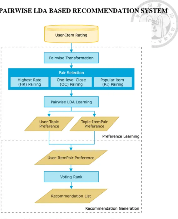
Figure 1.The pairwise LDA based recommendation system.

Figure 1 shows our pairwise LDA based recommendation system which consists of two stages: preference learning and recommendation generation. In the preference learning stage, we enhance LDA by considering item precedence to learn the implicit preferences of users. We examine the ratings of items made by users to construct precedence item pairs which reveal the users’ precedence over items. Three item pair selection strategies are developed that representative item pairs are selected to improve our pairwise LDA preference learning. The selected precedence item pairs are fed into

(13)

LDA to infer two model parameters, namely, the latent topic distributions of users and the item precedence distributions of topics. In the recommendation generation stage, a recommendation list is generated for a target user using a voting mechanism which computes the precedence of items in terms of the two distributions. In the following sub- sections, we first present our pairwise LDA preference learning and the selection strategies of precedence item pairs. Last, we detail the voting mechanism of item recommendations.

3.1 Preference Learning

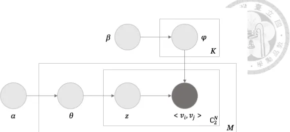
The goal of the preference learning is to derive users’ implicit preferences from their rating behavior. In contrast to most matrix-factorization-based recommendation methods which acquire user preferences by approximating users’ item ratings, we in this paper consider the precedence of items to learn user preferences. Specifically, we incorporate the concept of pairwise learning into LDA to learn user preferences. Figure 2 illustrates the graphical model of our pairwise LDA preference learning.

Generally, users are associated with a diversity of topics and each topic exhibits distinct preferences over items. For instance, teenagers tend to like action, adventure, and horror films, and therefore are likely to love the movie “Transformers” more than the documentary, crime movie “Inside Job.” On the other hand, adults are generally interested in genres like documentaries and biographies and would prefer to watch the documentary

“An Inconvenient Truth” instead of the horror movie “The Conjuring.” In our pairwise LDA preference learning, users and item precedence are linked by latent (implicit) topics, and a user’s preferences are expressed by a mixture of K topics. Let random variable z represent a topic and let U = {u1, u2, ..., uM} be a set of users. A user’s implicit preferences

(14)

Figure 2. The graphical model of the preference learning.

are modeled by a multinomial distribution over K topics and are expressed as a K dimensional topic vector 𝜃𝜃^(𝑚𝑚) such that vector element 𝜃𝜃_𝑘𝑘^(𝑚𝑚) indicates the association of um with a topic k, that is, 𝜃𝜃_𝑘𝑘^(𝑚𝑚)= P(z = k | um). To model a topic’s precedence on items, we characterize a topic as a multinomial distribution over item pairs. Let V = {v1, v2, ..., vN} be a set of items. We represent a topic as a probability vector 𝜑𝜑^(𝑘𝑘), where each vector dimension stands for an item precedence pair <vi, vj>. The vector element 𝜑𝜑_<𝑣𝑣^(𝑘𝑘)_𝑖𝑖_,𝑣𝑣_𝑗𝑗_> = P(<vi, vj>|z = k) reveals the likelihood that users in that topic prefer item vi over vj. Variables α and β are hyper-parameters of the LDA model and they characterize the symmetric Dirichlet priors of 𝜃𝜃^(𝑚𝑚) and 𝜑𝜑^(𝑘𝑘). With the two multinomial distributions, that is, 𝜃𝜃^(𝑚𝑚) and 𝜑𝜑^(𝑘𝑘), the likelihood that um prefers vi over vj can be computed by the following equation. Items can thus be ranked according to um’s preferences, and the recommendations of items are generated.

𝑃𝑃(< 𝑣𝑣_𝑖𝑖, 𝑣𝑣_𝑗𝑗> |𝑢𝑢_𝑚𝑚, 𝛼𝛼, 𝛽𝛽) = ∑ 𝑃𝑃�< 𝑣𝑣𝑘𝑘 𝑖𝑖, 𝑣𝑣_𝑗𝑗 > |𝑧𝑧 = 𝑘𝑘, 𝛽𝛽�𝑃𝑃�𝑧𝑧 = 𝑘𝑘|𝑢𝑢𝑚𝑚,𝛼𝛼� =∑ 𝜑𝜑_𝑘𝑘 _<𝑣𝑣^(𝑘𝑘)_𝑖𝑖_,𝑣𝑣_𝑗𝑗_>𝜃𝜃_𝑘𝑘^(𝑚𝑚). (1)

(15)

Many inference algorithms have been developed to estimate parameters of LDA.

Here, we adopt Gibbs sampling to obtain 𝜃𝜃^(𝑚𝑚) and 𝜑𝜑^(𝑘𝑘) through the item ratings made by users. Let variable rm,i denote the rating made by um on vi. For each user um, we form the collection of item precedence pairs 𝐶𝐶^(𝑚𝑚) = { <vi,vj> | rm,i > rm,j} that reflects um’s precedence over item pairs. After this, the item precedence pairs of all users ℂ = {𝐶𝐶⁽¹⁾, 𝐶𝐶⁽²⁾, …, 𝐶𝐶^(𝑀𝑀)} are applied to LDA to derive the distributions of 𝜃𝜃^(𝑚𝑚) and 𝜑𝜑^(𝑘𝑘).

Gibbs sampling is an implementation through Markov chain Monte Carlo (MCMC) (Gemman & Geman, 1984). It obtains model parameters by constructing a Markov chain that converges to the target distribution of that model. Then, samples from the Markov chain are used to estimate model parameters. In our pairwise LDA preference learning, each state of the Markov chain consists of the assignments of topics (i.e., z) to the item precedence pairs in ℂ. The Markov chain begins with an initial state in which every item precedence pair is randomly assigned a value between 1 to K, that is, the item pair’s topic.

Then, following Griffiths and Steyvers (2004), the state transition of the Gibbs sampling is conducted by sequentially sampling all item precedence pairs’ topics by means of the following posterior probability. Note that the topic sampling is conditioned on all other item precedence pairs and their topic assignments.

𝑃𝑃(𝑧𝑧𝑥𝑥 = 𝑘𝑘|𝑧𝑧−𝑥𝑥, ℂ) ∝^𝑛𝑛^{−𝑥𝑥,𝑘𝑘}<𝑣𝑣𝑖𝑖,𝑣𝑣𝑗𝑗>𝑥𝑥+𝛽𝛽

𝑛𝑛_{−𝑥𝑥,𝑘𝑘}^∗ +�|ℂ|�𝛽𝛽∗ ^𝑛𝑛^{−𝑥𝑥,𝑘𝑘}^{𝑢𝑢{𝑥𝑥}}^+𝛼𝛼

𝑛𝑛_−𝑥𝑥^{𝑢𝑢{𝑥𝑥}}+𝐾𝐾𝛼𝛼, (2)

where zx stands for the topic of the x’th (i.e., the current sampling) item precedence pairs in ℂ, and z^-x denotes all the item precedence pairs’ topics, excluding the current one.

Symbol <vi,vj>x denotes the item precedence pair of the current sampling, and 𝑛𝑛_{−𝑥𝑥,𝑘𝑘}^<𝑣𝑣^𝑖𝑖^,𝑣𝑣^𝑗𝑗^>^𝑥𝑥 is the number of times that <vi,vj>x is assigned to topic k, not including the current

(16)

item pair. Also, 𝑛𝑛_{−𝑥𝑥,𝑘𝑘}^∗ is the number of item pairs assigned to topic k, not including the current sampling. ||ℂ|| is the number of unique item pairs in ℂ. Finally, u^{x} represents the user from whom the item precedence pair of the current sampling comes. Then, 𝑛𝑛_{−𝑥𝑥,𝑘𝑘}^𝑢𝑢^{𝑥𝑥} is the number of u{x}’s item pairs assigned to topic k, not including the current one, and 𝑛𝑛_−𝑥𝑥^𝑢𝑢^{𝑥𝑥}is the number of u{x}’s item pairs, not including the current sampling.

With a sufficient number of state transitions, the Markov chain reaches a stationary distribution and maximize the log likelihood. Log likelihood is defined as follow,

𝐿𝐿𝐿𝐿𝐿𝐿 𝐿𝐿𝐿𝐿𝑘𝑘𝐿𝐿𝐿𝐿𝐿𝐿ℎ𝐿𝐿𝐿𝐿𝑜𝑜 = ∑_{𝑢𝑢∈𝑈𝑈}∑_<𝑣𝑣_𝑖𝑖_,𝑣𝑣_𝑗𝑗_>∈ℂ_𝑢𝑢log ∑_{𝑘𝑘∈𝐾𝐾}𝜃𝜃_𝑘𝑘^(𝑢𝑢)𝜑𝜑_<𝑣𝑣^(𝑘𝑘)_𝑖𝑖_,𝑣𝑣_𝑗𝑗_>. (3)

Since 1 and 0 represent the probability of the appearance of the pair, maximize the log likelihood means the probability of every rated items have been approximated to 1.

We then use its current topic assignments to estimate 𝜃𝜃^(𝑚𝑚) and 𝜑𝜑^(𝑘𝑘) as follows.

𝜃𝜃_𝑘𝑘^(𝑚𝑚) = 𝑛𝑛_𝑘𝑘^𝑢𝑢^𝑚𝑚+ 𝛼𝛼

𝑛𝑛_∗^𝑢𝑢^𝑚𝑚+ 𝐾𝐾𝛼𝛼 (4)

and

𝜑𝜑_<𝑣𝑣^(𝑘𝑘)_𝑖𝑖_,𝑣𝑣_𝑗𝑗_> = ^𝑛𝑛^𝑘𝑘<𝑣𝑣𝑖𝑖,𝑣𝑣𝑗𝑗>+𝛽𝛽

𝑛𝑛_𝑘𝑘^∗+||ℂ||𝛽𝛽, (5)

where 𝑛𝑛_𝑘𝑘^𝑢𝑢^𝑚𝑚 is the number of um’s item precedence pairs that belong to topic k, and 𝑛𝑛_∗^𝑢𝑢^𝑚𝑚 is the count of um’s item precedence pairs. Symbol 𝑛𝑛_𝑘𝑘^<𝑣𝑣^𝑖𝑖^,𝑣𝑣^𝑗𝑗^> is the number of times that <vi, vj> is assigned to topic k, and 𝑛𝑛_𝑘𝑘^∗ is the count of item precedence pairs assigned to topic k.

(17)

3.2 Strategies of Item Precedence Pair Selection

The pairwise LDA preference learning collects item precedence pairs to derive the distributions 𝜃𝜃^(𝑚𝑚) and 𝜑𝜑^(𝑘𝑘). However, including non-representative precedence pairs into the learning process could deteriorate the learned distribution that subsequently affects our recommendation performance. Here, we develop three strategies to select representative precedence pairs for effective preference learning. Learning with the selected precedence pairs could improve the learned preference distributions. Besides, the preference learning process is accelerated because the size of the training data is reduced.

Strategy 1: Highest Rate (HR) Pairing

Given an item ranking list, users often focus top few items (Lam & Riedl, 2004). So, the learned user preferences should be able to discriminate the favorable items of users from all other items. Because the user only cares about the first few items in the recommendation list, it is recommended that if the list exceeds a certain length, the probability of item behind being seen by the user is very low. Therefore, it is not necessary to accurately predict low ranking items (ex to find items that may be rated 2 and items that may be rated 1).

Also, we noticed that the item precedence pairs collected in Section 3.1 comprise pairs irrelevant to user preferences. For instance, if a user had rated items vi and vj as 2 and 1, respectively, the item precedence pair <vi, vj> would be collected to learn um’s preference (i.e., 𝜃𝜃^(𝑚𝑚)) even though the user does not like any of the items. To learn user preferences from preferable items, the highest rate pairing strategy identifies the set of items that obtained the highest rate of a user. The items are regarded as the favorable items of the user and are paired with the remaining rated items of the user to construct the item precedence pairs.

(18)

Strategy 2: One-Level Close (OC) Pairing

Lin et al (2013) studied the selection of data points for effective support vector machine learning. They demonstrated that data points of different categories (classes) are helpful to machine learning if they are close to each other in the vector space. Data points are close when they have similar features. It is difficult to classify these close points if they belong to different categories. These data points thus are crucial to deduce effective machine learning models. In terms of our item precedence pair selection, we consider any two items whose ratings are with a one-level difference as close data points because they reveal subtle difference in user preferences. The one-level close strategy then selects all these item pairs to learn the preference distributions.

Strategy 3: Popular Item (PI) Pairing

The revenue of e-commerce platforms mostly comes from the sales of popular items, which is known as 80/20 rule. While the word of mouth effect on the Internet increases the exposure of non-popular products, it also increases the demand of popular items that the top 20% popular items contribute 80% revenue of e-commerce (Tan, 2009). It is therefore essential to learn user preference from popular items. We design the popular item pairing strategy which identifies a set of popular items that have received a lot of ratings. Then, precedence item pairs are constructed by pairing all the items in the set.

3.3 Recommendation Generation

In the recommendation generation stage, we use the distributions 𝜃𝜃^(𝑚𝑚) and 𝜑𝜑^(𝑘𝑘)to generate item recommendations for users. By taking the distributions into Equation 1, we compute the probability that a user um prefers an item vi over vj. Ideally, we can use the probability to rank items and suggest the top items to users. However, the pairwise precedence described by the equation may not be transitive, and for this reason, we may

(19)

not be able to produce a unique ranking for the items. To resolve this problem, we consider a weighted voting scheme for pairwise preferences (Fürnkranz et al., 2008), and in this way, for each item vi, we use the following equation to compute its voting weight.

𝑅𝑅𝑚𝑚(𝑣𝑣𝑖𝑖) = ∑𝑣𝑣_𝑗𝑗≠𝑣𝑣_𝑖𝑖𝑃𝑃(< 𝑣𝑣𝑖𝑖, 𝑣𝑣𝑗𝑗 > |𝑢𝑢𝑚𝑚), (6)

where Rm(vi) stands for the voting score of item vi. Basically, the score of an item is the sum of its precedence probabilities over all other items. The larger the value is, the more likely that um prefers vi. Then, we rank items according to their voting scores and the top- ranked items are suggested to the target user.

4 EXPERIMENT

4.1 Datasets and Evaluation Metrics

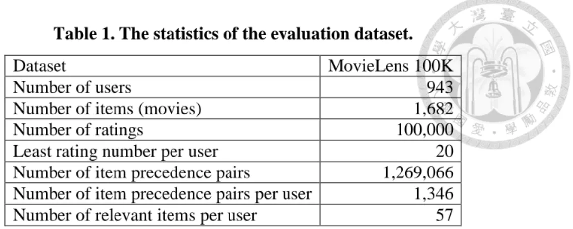
To evaluate the purposed method, we conducted experiments using the MovieLens 100K dataset¹ which consists of 100,000 ratings made by 943 users across 1,682 movies.

We selected the dataset for evaluations because it contains abundant rating information, hence it is widely used by many recommendation evaluations (Guo et al., 2013; Li et al., 2015). Table 1 details the statistics of the evaluation dataset.

We adopted the conventional 5-fold cross validation (Kohavi, 1995) to obtain fair evaluation results. Specifically, system performance is evaluated in 5 runs that they evenly partitioned users’ ratings into 5 folds. Each validation run takes the ratings of one fold as the testing data (i.e., the ground truth). The remaining 4 folds are used to learn us-

1 https://grouplens.org/datasets/movielens/100k/

(20)

Table 1. The statistics of the evaluation dataset.

er preferences and to recommend items to the users. Four metrics including the precision rate at k, R-precision (Larson, 2010), mean reciprocal rank (Voorhees, 1999), and diversity at k (Adomavicius & Kwon, 2012) are applied to the recommended items and the testing ratings to evaluate the recommendation results. The results of the 5 runs are then averaged to obtain the global recommendation performance.

In our experiments, a recommended item is relevant to a user’s interests if the item’s rating made by the user is included in the testing data and the rating is above the average rating of that user. The precision at k (denoted as P@K) defined below calculates the fraction of the top k recommended items that a user is interested in. The higher the value, the better the recommendation performance is. We noticed the number of relevant items varies among users and the variation would affect the precision at k (Larson, 2010). To lessen of the influence, we examine P@K under different settings of k. Also, we evaluate recommendation performance using the R-precision which is a variant of P@K that k is equal to the number of relevant items rated by a user.

P@K = 1

|𝑈𝑈| �

|# 𝐿𝐿𝑜𝑜 𝑟𝑟𝐿𝐿𝐿𝐿𝐿𝐿𝑣𝑣𝑟𝑟𝑛𝑛𝑟𝑟 𝐿𝐿𝑟𝑟𝐿𝐿𝑖𝑖𝑖𝑖 𝐿𝐿𝑛𝑛 𝑟𝑟ℎ𝐿𝐿 𝑟𝑟𝐿𝐿𝑡𝑡 𝐾𝐾 𝑟𝑟𝐿𝐿𝑟𝑟𝐿𝐿𝑖𝑖𝑖𝑖𝐿𝐿𝑛𝑛𝑜𝑜𝐿𝐿𝑜𝑜 𝐿𝐿𝑟𝑟𝐿𝐿𝑖𝑖𝑖𝑖|

u∈𝑈𝑈 𝐾𝐾

. (7)

Dataset MovieLens 100K

Number of users 943

Number of items (movies) 1,682

Number of ratings 100,000

Least rating number per user 20

Number of item precedence pairs 1,269,066 Number of item precedence pairs per user 1,346

Number of relevant items per user 57

(21)

The mean reciprocal rank (MRR) defined below is a well-known ranking quality metric.

MRR = 1

|𝑈𝑈| � max^{𝑣𝑣∈𝑅𝑅}^𝑢𝑢 1 𝑟𝑟𝑟𝑟𝑛𝑛𝑘𝑘𝑣𝑣 u∈𝑈𝑈

, (8)

where Ru represents the set of user u’s relevant items and 𝑟𝑟𝑟𝑟𝑛𝑛𝑘𝑘𝑣𝑣 is the position of the item v in the recommendation list. A high MRR means that the recommendation system is able to place items relevant to user interests to the top of a recommendation list. Finally, the diversity at k is defined as follows.

diversity@𝑘𝑘^{= �� 𝐿𝐿}𝐾𝐾(𝑢𝑢)

𝑢𝑢∈𝑈𝑈

�, (9)

where LK(u) represents the set of top K items recommended to user u. Unlike the above metrics that they concern the relevance of the recommended items, diversity at k

examines the number of different items recommended to users. A high diversity at k

indicates the recommendations are diverse because users receive different item suggestions.

4.2 Effect of System Parameters

We adopted the GibbsLDA++ package² to implement our preference learning which consists of three system parameters, K, 𝛼𝛼, and 𝛽𝛽. Parameters 𝛼𝛼 and 𝛽𝛽 are the hyper- parameters of the LDA priors, and K determines the number of latent topics. As mentioned in Section 3.1, the learning process is based on the Gibbs sampling which is an iterative procedure that sequentially labels the topics of the item precedence pairs to

2 http://gibbslda.sourceforge.net

(22)

maximize the likelihood of Equation 3. Here, we examine the effect of the parameters on the negative log likelihood value that a good parameter setting would produce a low negative log likelihood.

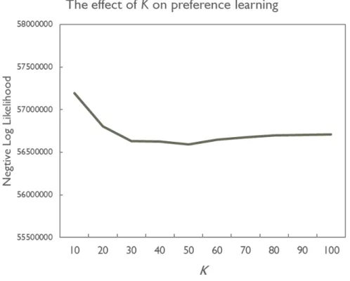
Figure 3 shows the effect of K. Here, the parameters 𝛼𝛼 and 𝛽𝛽 are set at 0.1 and 0.05, respectively. Later, we examine their effects. The x-coordinate of the figure is the number of the latent topics (i.e., K) and the y-coordinate designates the negative log likelihood. As shown in the figure, a small K (e.g., 10 or 20) produces to a poor negative log likelihood. This is because movies are generally associated diverse categories that a small K may not be able to express the movies correctly. The negative log likelihood improves as K increases, and the likelihood turns into stable when K is greater or equal to 30. We therefore set K at 30 in the following experiments.

Figure 3. The effect of K on the negative log likelihood.

(23)

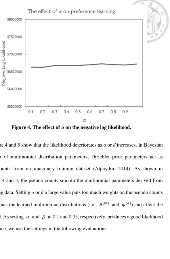
Figure 4. The effect of α on the negative log likelihood.

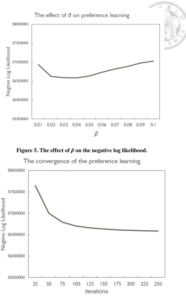
Figure 4 and 5 show that the likelihood deteriorates as α or β increases. In Bayesian estimation of multinomial distribution parameters, Dirichlet prior parameters act as pseudo counts from an imaginary training dataset (Alpaydin, 2014). As shown in Equations 4 and 5, the pseudo counts smooth the multinomial parameters derived from the training data. Setting α or β a large value puts too much weights on the pseudo counts that thus bias the learned multinomial distributions (i.e., 𝜃𝜃^(𝑚𝑚) and 𝜑𝜑^(𝑘𝑘)) and affect the likelihood. As setting 𝛼𝛼 and 𝛽𝛽 at 0.1 and 0.05, respectively, produces a good likelihood performance, we use the settings in the following evaluations.

(24)

Figure 5. The effect of β on the negative log likelihood.

Figure 6. The convergence of the preference learning.

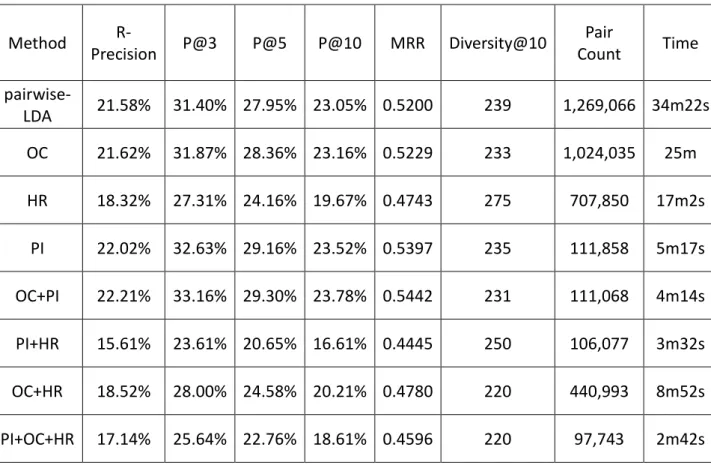
Last, we examine the convergence of the iterative Gibbs sampling using the above

(25)

parameter settings. In our experiment, the evaluation dataset is huge and it comprises 1,269,066 item precedence pairs (see Table 1). Nevertheless, the likelihood rapidly converges around 100 iterations as shown in Figure 6. The result indicates that our preference learning is feasible to real world e-commerce platforms and is able to learn user preference efficiently.

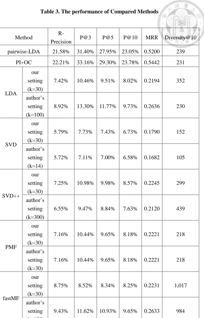
4.3 Examination of Strategies

Table 2 compares the recommendation performance with and without using the item precedence pair selection strategies. To detail the benefit of the strategies, the table also lists the number of selected precedence pairs of each strategy. It is noteworthy that the P@K, R-precision, and MRR scores are all low. This is because the metrics are based on the rated items. As shown in table 1, an evaluated user only rated about at least 20 items and the dataset contains 1,682 recommendable items. Suggesting favorable items thus is not easy. Nevertheless, our method still outperforms many well-known recommendation methods as shown in the next section.

While using the strategies decreases a great number of precedence pairs, the corresponding performances are still comparable to those without using them. The result indicates that the designed strategies are able to select representative precedence pairs.

Also, by reducing the number of precedence pairs, the strategies help accelerate the preference learning process. For instance, under the PI strategy, the precedence pair number is decreased from 1,269,066 to 111,858 that dramatically speeds up the learning process from 34 minutes and 22 seconds to 5 minutes and 17 seconds.

The PI strategy achieves superior recommendation performance. The result indicates that the strategy is good at distinguishing the preferences of users on popular items.

(26)

However, as it mainly focuses on popular items, its diversity (e.g., diversity at k) is low.

Because popular items normally contribute around 80% revenues of e-commerce, this strategy is valuable. Intuitively, HR should be able to produce good item recommendation because it is based on the items that the users most preferred. On the other hand, OC should be inferior because it could include minor precedence pairs into the learning process. For instance, if a user gave several items low ratings, like 2 and 1, the precedence pairs would comprise these disfavor items that would bias the learned preference distributions. Contrary to our expectations, OC has a fine performance and HR performs poorly. To reason the outcome, we calculated the average rating made by the evaluated users, which is 3.59 with a narrow standard deviation of 0.44. In other words, the users tend to give items a high rating. The pairs selected by OC thus focus on the items favored

Table 2.The result of pair selection.

Method R-

Precision P@3 P@5 P@10 MRR Diversity@10 Pair

Count Time pairwise-

LDA 21.58% 31.40% 27.95% 23.05% 0.5200 239 1,269,066 34m22s OC 21.62% 31.87% 28.36% 23.16% 0.5229 233 1,024,035 25m HR 18.32% 27.31% 24.16% 19.67% 0.4743 275 707,850 17m2s

PI 22.02% 32.63% 29.16% 23.52% 0.5397 235 111,858 5m17s OC+PI 22.21% 33.16% 29.30% 23.78% 0.5442 231 111,068 4m14s PI+HR 15.61% 23.61% 20.65% 16.61% 0.4445 250 106,077 3m32s OC+HR 18.52% 28.00% 24.58% 20.21% 0.4780 220 440,993 8m52s PI+OC+HR 17.14% 25.64% 22.76% 18.61% 0.4596 220 97,743 2m42s

(27)

by the users; so it produces a good recommendation performance. Regarding the poor performance of HR, we noticed that users’ HR precedence pairs are complete different unless they have the same highest rated items. The phenomenon disturbs the learned preference distributions (i.e., 𝜃𝜃^(𝑚𝑚)) if the items they rated overlap greatly. For instance, if um‘s ratings on items vw, vx, vy, and vz are 5, 4, 3, and 2, and un’s ratings on vx, vy, and vz

are 4, 3, and 2. Even though the two users have the same tastes on vx, vy, and vz, their HR precedence pairs have no overlap. As the overlap between the non-highest rated items is overlooked, HR’s recommendations are inferior.

We also evaluate the combination of the strategies by intersect the pairs they selected.

Due to the disadvantage of HR, the approaches that combine HR are inferior. Note that our method achieves the best performance by combining PI and OC. As the two strategies select precedence pairs from different perspectives, combining them is helpful in improving our preference learning.

4.4 Comparisons with Other Recommendation Methods

We compare our method with the following five well-known model based recommendation methods.

 SVD (Sarwar et al., 2000) is a matrix factorization algorithm that factorizes a user- item rating matrix into the user preference matrix and the item preference matrix.

The preference matrices are used to identify a set of like-minded users and to predict the rating of an item for a target user.

 SVD++ (Koren., 2008) enhances the SVD method by examining implicit user feedbacks on items. The method constructs a binary matrix indicating whether a user

(28)

has rated an item. The binary matrix is regarded as the implicit user feedback and is combined with the explicit ratings to estimate latent preferences.

 PMF (Mnih & Salakhutdinov, 2008) is a probabilistic extension of SVD. The authors presumed the preferences (ratings) of users on items are determined by a probabilistic linear model that incorporates a Gaussian prior distribution to minimize the root mean squared error of the predicted ratings. The evaluation shows that the method is effective when ratings are sparse.

 LDA (Xie & Gao, 2014) applies the latent Dirichlet allocation to learn user preferences from ratings. Different to our method, the learning process does not consider the precedence between items. Comparing this method helps realize the benefit of our pairwise learning.

 fastMF (He et al., 2016) improves matrix factorization approaches by assigning weights to missing ratings. Many recommendation systems discard missing ratings of items by assuming that users do not notice the items. However, if the items are popular items, the missing ratings may be a hint that the users do not like the items.

The fastMF assigns different weights to items according to item popularity. Also an alternating least squares technique is adopted to enhance the efficiency of the matrix factorization.

(29)

Table 3. The performance of Compared Methods

Method R-

Precision P@3 P@5 P@10 MRR Diversity@10 pairwise-LDA 21.58% 31.40% 27.95% 23.05% 0.5200 239

PI+OC 22.21% 33.16% 29.30% 23.78% 0.5442 231

LDA

our setting (k=30)

7.42% 10.46% 9.51% 8.02% 0.2194 352 author’s

setting (k=100)

8.92% 13.30% 11.77% 9.73% 0.2636 230

SVD

our setting (k=30)

5.79% 7.73% 7.43% 6.73% 0.1790 152 author’s

setting (k=14)

5.72% 7.11% 7.00% 6.58% 0.1682 105

SVD++

our setting (k=30)

7.25% 10.98% 9.98% 8.57% 0.2245 299 author’s

setting (k=300)

6.55% 9.47% 8.84% 7.63% 0.2120 439

PMF

our setting (k=30)

7.16% 10.44% 9.65% 8.18% 0.2221 218 author’s

setting (k=30)

7.16% 10.44% 9.65% 8.18% 0.2221 218

fastMF

our setting (k=30)

8.75% 8.52% 8.34% 8.25% 0.2231 1,017 author’s

setting (k=128)

9.43% 11.62% 10.93% 9.65% 0.2633 984

(30)

To ensure the comparisons are fair, the compared methods were implemented with public domain packages³. Besides, the same 5-fold cross validation is applied to the methods to obtain their recommendation performance. Regarding to the number of latent topics, we evaluated the methods by settings K at 30. We also test their performance under the K suggested by the authors.

As shown in Table 3, our method dominates the compared methods in terms of R- precision, P@K, and MRR. Normally, P@K decreases as K increases. This is because the items are ranked according to their relevance to user preferences. A large K thus includes false item suggestions that affect the precision performance. The P@K scores of the compared methods are low. In other words, the methods are not able to place items relevant to user preferences at the top of the recommendation list. As a result, their MRRs are all inferior. By contrast, our precision performances are good that the MRR scores are almost double to theirs.

The SVD, SVD++, PMF, and fastMF methods are all matrix factorization approaches that their preference learning aims at minimizing the difference between the predicted ratings and the ratings given by users. As shown in Table 3, SVD++, PMF, and fastMF performance better than SVD does. This is because the methods enhance SVD by means of various item information (e.g., the popularity of items to weight missing ratings).

Nevertheless, their performances are still inferior to ours. Essentially, the goal of recommendation systems is to rank items according to user preference (Pessiot et al., 2007). Rather than approximating the ratings given by users, our preference learning

3 For PMF, SVD, and SVD++, we used the Surprise matrix factorization package (http://surprise.readthedocs.io/en/stable/index.html). FastMF was based on the authors’

code released on https://github.com/hexiangnan/sigir16-eals.

(31)

examines the precedence of items to obtain user preferences. The superior performance of our method validates the value of our pairwise learning. The LDA method and our method are graphical model approaches that our method further considered item precedence to acquire user preferences. The improvement of our method over LDA again demonstrates the benefit of our pairwise learning.

Except fastMF, all the methods produce low diversity scores. As shown in Table 1, the users in the evaluation dataset only rated at least 20 items out of 1,682 items. The rating sparsity phenomenon severely affects the ability of the methods to recommend items received little or no ratings. Consequently, the methods’ diversity performances are poor. As mentioned above, fastMF assigns weights to missing ratings. The method thus is able to recommend different items and achieves good diversity performance.

In summary, our method is superior to the state-of-art methods in R-precision, P@K, and MRR. Our method was able to recommend items that has potential to be rated high scores. By increasing the probability of items exposure, users’ satisfaction is increase and items provider achieve higher loyalty from their users.

5 DISCUSSIONS AND IMPLICATIONS

In this paper, we have developed an effective recommendation method that combines pairwise learning with latent Dirichlet allocation. Instead of approximating the ratings of items made by users, the method examines the precedence between items to learn user preferences. In addition, pair selection strategies are designed to select representative item precedence pairs. The experiment results based on a huge dataset show that the strategies make our preference learning effective and efficient. Moreover, the proposed pairwise

(32)

LDA recommendation method outperforms the state-of-the-art recommendation methods in terms of R-precision, precision at k, and MRR.

Our study reveals several potential research directions. First, the experiment result shows that the recommendations based on primitive LDA is comparable to those of the sophisticated matrix factorization methods. While the research of recommendation systems primarily focused on enhancement of matrix factorization, the result suggests that graphical models that associate user behavior (e.g., ratings) with their preferences in probability theory are promising. Second, by considering pairwise learning, our method enhances LDA significantly. The superior performance of our method also suggests recommendation system researchers adopt learning to rank techniques to improve recommendation performance. This suggestion also corresponds to Pessiot et al. (2007)’s assertion that the core of recommendation systems is to rank items according to user preference, rather approximating the ratings given by users. Regarding the precedence pair selection strategies, our study indicates that not only popular items but also item pairs that reveal subtle preference differences of users are informative to recommendation systems. Notably, the strategies help our recommendations concentrate on popular items.

As the revenue of e-commerce is normally based on the sales of popular items. Our evaluation results also encourage researchers to investigate popular item recommendations.

6 LIMITATIONS AND FUTURE WORKDS

Our research is subject to the following limitations. First, as our preference learning is based on the precedence of items, we cannot learn the preference of a user if the user gave all the rated items the same rating. In the future work, we will investigate the missing

(33)

not at random (Marlin & Zemel, 2009) which examines the preference of users against non-rating items. We would give different weights (e.g., ratings) to items that are ignored by a user according to the item popularity. This way, item precedence pairs could be generated to derive user preferences. Second, while our method is good at recommending popular items, the diversity of the recommendations is low. This is because the Gibbs sampling is a frequency based inference algorithm that unpopular items may receive a low recommendation probability. As mentioned above, we will investigate a weighting scheme to assign weights to missing items. The weight scheme will also revise the weight of popular and unpopular items so as to increase the chance of suggesting unpopular items.

Moreover, as the preferences of users may be affected by friends, social influence will be incorporated into the preference inference procedure to increase the recommendation diversity.

7 REFERENCES

 Adomavicius, G. and Y. Kwon (2012). "Improving aggregate recommendation diversity using ranking-based techniques." IEEE Transactions on Knowledge and Data Engineering 24(5): 896-911.

 Aggarwal, C. C. (2016). Recommender systems, Springer.

 Alpaydin, E. (2014). Introduction to machine learning, MIT press.

 Blei, D. M., et al. (2003). "Latent dirichlet allocation." Journal of machine Learning research 3(Jan): 993-1022.

 Breese, J. S., et al. (1998). Empirical analysis of predictive algorithms for

collaborative filtering. Proceedings of the Fourteenth conference on Uncertainty in artificial intelligence, Morgan Kaufmann Publishers Inc.

 Deshpande, M. and G. Karypis (2004). "Item-based top-n recommendation

(34)

algorithms." ACM Transactions on Information Systems (TOIS) 22(1): 143-177.

 Fürnkranz, J., et al. (2008). "Multilabel classification via calibrated label ranking."

Machine learning 73(2): 133-153.

 Gemman, S. and D. Geman (1984). "Stochastic relaxation, Gibbs Distributions, and The Bayesian of Images." IEEE Trans. Pattern Anal. Mach. Intelligence 6.

 Gemulla, R., et al. (2011). Large-scale matrix factorization with distributed stochastic gradient descent. Proceedings of the 17th ACM SIGKDD international conference on Knowledge discovery and data mining, ACM.

 Griffiths, T. L. and M. Steyvers (2004). "Finding scientific topics." Proceedings of the National academy of Sciences 101(suppl 1): 5228-5235.

 Guo, G., et al. (2013). A Novel Bayesian Similarity Measure for Recommender Systems. IJCAI.

 He, X., et al. (2016). Fast matrix factorization for online recommendation with implicit feedback. Proceedings of the 39th International ACM SIGIR conference on Research and Development in Information Retrieval, ACM.

 Kohavi, R. (1995). A study of cross-validation and bootstrap for accuracy estimation and model selection. Ijcai, Montreal, Canada.

 Koren, Y. (2008). Factorization meets the neighborhood: a multifaceted

collaborative filtering model. Proceedings of the 14th ACM SIGKDD international conference on Knowledge discovery and data mining, ACM.

 Koren, Y., et al. (2009). "Matrix factorization techniques for recommender systems." Computer 42(8).

 Lai, H.-J., et al. (2003). Customized internet news services based on customer profiles. Proceedings of the 5th international conference on Electronic commerce, ACM.

(35)

 Lam, S. K. and J. Riedl (2004). Shilling recommender systems for fun and profit.

Proceedings of the 13th international conference on World Wide Web, ACM.

 Larson, R. R. (2010). "Introduction to information retrieval." Journal of the American Society for Information Science and Technology 61(4): 852-853.

 Li, S., et al. (2015). Deep collaborative filtering via marginalized denoising auto- encoder. Proceedings of the 24th ACM International on Conference on Information and Knowledge Management, ACM.

 Li, Z. and C. Xu (2013). Tag-based top-N recommendation using a pairwise topic model. Information Reuse and Integration (IRI), 2013 IEEE 14th International Conference on, IEEE.

 Lin, K.-Y., et al. (2013). Data selection techniques for large-scale rank SVM.

Technologies and Applications of Artificial Intelligence (TAAI), 2013 Conference on, IEEE.

 Lops, P., et al. (2011). Content-based recommender systems: State of the art and trends. Recommender systems handbook, Springer: 73-105.

 Marlin, B. M. and R. S. Zemel (2009). Collaborative prediction and ranking with non-random missing data. Proceedings of the third ACM conference on

Recommender systems, ACM.

 Mnih, A. and R. R. Salakhutdinov (2008). Probabilistic matrix factorization.

Advances in neural information processing systems.

 Pessiot, J.-F., et al. (2007). "Learning to rank for collaborative filtering."

 Rendle, S., et al. (2009). BPR: Bayesian personalized ranking from implicit feedback. Proceedings of the twenty-fifth conference on uncertainty in artificial intelligence, AUAI Press.

 Resnick, P., et al. (1994). GroupLens: an open architecture for collaborative

(36)

filtering of netnews. Proceedings of the 1994 ACM conference on Computer supported cooperative work, ACM.

 Sarwar, B., et al. (2000). Application of dimensionality reduction in recommender system-a case study, Minnesota Univ Minneapolis Dept of Computer Science.

 Sarwar, B., et al. (2001). Item-based collaborative filtering recommendation algorithms. Proceedings of the 10th international conference on World Wide Web, ACM.

 Sharma, A. and B. Yan (2013). Pairwise learning in recommendation: experiments with community recommendation on linkedin. Proceedings of the 7th ACM Conference on Recommender Systems, ACM.

 Shi, Y., et al. (2010). List-wise learning to rank with matrix factorization for collaborative filtering. Proceedings of the fourth ACM conference on

Recommender systems, ACM.

 Tan, T. F. and S. Netessine (2009). "Is Tom Cruise threatened? Using Netflix Prize data to examine the long tail of electronic commerce." Wharton Business School, University of Pennsylvania, Philadelphia.

 Voorhees, E. M. (1999). The TREC-8 Question Answering Track Report. Trec.

 Wang, J., et al. (2006). Unifying user-based and item-based collaborative filtering approaches by similarity fusion. Proceedings of the 29th annual international ACM SIGIR conference on Research and development in information retrieval, ACM.

 Xie, W., et al. (2014). "A probabilistic recommendation method inspired by latent dirichlet allocation model." Mathematical Problems in Engineering 2014.

 Yao, W., et al. (2015). Collaborative Topic Ranking: Leveraging Item Meta-Data for Sparsity Reduction. AAAI.

 Yu, K., et al. (2004). "Probabilistic memory-based collaborative filtering." IEEE

(37)

Transactions on Knowledge and Data Engineering 16(1): 56-69.

 Zhang, B.-T. and Y.-W. Seo (2001). "Personalized web-document filtering using reinforcement learning." Applied Artificial Intelligence 15(7): 665-685.