中国生态系统研究网络

(1)

BGD

6, 2913–2937, 2009

Comparison of CO₂ fluxes in a subtropical

ecosystem J.-H. Yan et al.

Title Page Abstract Introduction Conclusions References

Tables Figures

J I

Back Close

Full Screen / Esc

Printer-friendly Version Interactive Discussion

Biogeosciences Discuss., 6, 2913–2937, 2009 www.biogeosciences-discuss.net/6/2913/2009/

Biogeosciences Discussions

Biogeosciences Discussions is the access reviewed discussion forum of Biogeosciences

A comparison of CO ₂ fluxes via eddy covariance measurements with model predictions in a dominant subtropical forest ecosystem

J.-H. Yan¹, G.-Y. Zhou¹, Y.-L. Li¹, D.-Q. Zhang¹, D. Otieno², and J. Tenhunen²

1South China Botanic Garden, Chinese Academy of Sciences, GuangZhou 510650, PR, China

2Department of Plant Ecology, University of Bayreuth, 95440 Bayreuth, Germany

Received: 11 February 2009 – Accepted: 23 February 2009 – Published: 11 March 2009 Correspondence to: Y.-L. Li ([email protected])

Published by Copernicus Publications on behalf of the European Geosciences Union.

(2)

BGD

6, 2913–2937, 2009

Tables Figures

J I

Back Close

Full Screen / Esc

Abstract

CO₂ fluxes were measured continuously for twelve months (2003) using eddy covariance technique at canopy layer in a dominant subtropical forest in South China. Our results showed that daytime maximum CO₂fluxes of the whole ecosystem varied from

−15 to −20 µmol m⁻²s⁻¹. The peaks of CO₂fluxes appeared earlier than the peaks of

5

solar radiation. Contribution of CO₂fluxes in a subtropical forest in the dry season was 53% of the annual total from the whole forest ecosystem. Daytime CO₂ fluxes were very large in October, November and December, which was therefore an important stage for uptake of CO₂by the forest ecosystem from the atmosphere.

Using the estimates of biomass, soil carbon and parameters of leaf photosynthesis

10

from other studies at the same forest, we ran a process-based model, CBM (stands for CSIRO Biosphere Model) for this site, and compared the predicted fluxes of CO₂with measurements. We obtained reasonable agreement. The mean difference between the simulated and measured daytime CO₂ fluxes from the year-round (8249 records) was −0.2 µmol m⁻²s⁻¹and implied well within measurement accuracy.

15

Based on estimates of forest ecosystem respiration, NEE was calculated −242 and −276 gCm⁻²year⁻¹ for measured and modelled, respectively. In previous study, NPP for this forest stand was 694 gCm⁻²year⁻¹ during 2003/04 and litterfall was 424 gCm⁻²year⁻¹. We therefore calculated NEE as −270 gCm⁻²year⁻¹and very similar to the values obtained by measured and modelled CO₂fluxes in this study.

20

1 Introduction

A recent study using biomass inventory data from China suggests that all forests in China are weak carbon sources, with an emission rate of 0.022 Pg C year⁻¹. Natural forests in China are estimated to be small carbon sinks, with 0.1 Pg C during the past decade (Fang et al., 2001). Research conducted during the last few years however,

25

indicate that subtropical forests play a major role in CO₂ uptake due to their mature

(3)

BGD

6, 2913–2937, 2009

Tables Figures

J I

Back Close

Full Screen / Esc

vegetation surfaces and also because of their evergreen nature (Zhou et al., 2006; Yan et al., 2006).

CO₂ is a major constituent of the greenhouse gases and its concentration in the atmosphere is directly influenced by human activities (Rannik et al., 2002), with significant impact on global climate. Recent studies have confirmed the important role

5

played by terrestrial vegetation in the current global climate change, particularly, the role of forests in the global carbon cycle (GCN, 1995). Thus, ecologists have an important role in evaluating CO₂ fluxes from terrestrial ecosystems. Previous studies have relied on chamber techniques or cuvettes to evaluate leaf-level or ecosystem level CO₂ exchange processes of vegetation communities (Edwards and Sollins, 1973; Keller et

10

al., 1986). However, such techniques are inherently limited, since they alter the local environment (Dennis et al., 1988). Of course, it is impossible to employ chambers for observing net CO₂ fluxes from forest canopy and long-term, continuous measurements to obtain statistically reliable results. Eddy covariance provides an alternative means for measuring CO₂ fluxes between the biosphere and the atmosphere. It is a

15

non-invasive and non-destructive micrometeorological method which reveals continuous integrated signals with low spatial (typically 0.05 to 1 km²) but high time resolution (usually 0.5 h). Gas exchange is measured at ecosystem or even landscape scale. It is a sound way to evaluate CO₂ uptake by the forest. Most of the flux towers have been established in North America, Europe and a few in Australia, Japan and South

20

Korea. Tower measurements of CO₂ fluxes over the dominant subtropical forest have been made since 2002 in South China by direct eddy covariance method within the Chinaflux network. Understanding the gas-exchange processes between the vegeta- tions and the atmosphere is extremely important in global biogeochemical cycles and also in predicting future climate change.

25

China’s subtropical zone has unique features, which include: (1) humid and warm climate, contrary to other regions at the same latitude around the globe that are extremely arid. (2) Long disturbance history, with intensive human activity in large areas that have left almost no mature forest. (3) The most rapid industrialization in China

(4)

BGD

6, 2913–2937, 2009

Tables Figures

J I

Back Close

Full Screen / Esc

during the past 20 years, especially in the southern part of the country, but accompa- nied by the creation of large areas of young forest or rapid conversion of bare land in mountainous areas into forest. (4) Presence of evergreen broad-leaved forest, which must differ significantly from other forests in terms of the carbon cycle. Considerable uncertainties, however, exist regarding the carbon budget in the subtropical forests of

5

Southern China despite several previous studies of the country’s forest carbon budgets using forest inventory data (Fang and Chen, 2001; Wang et al., 2001) and process - based models (Cao et al., 2003).

Dinghushan ecological station was established as a part of the Network of Biosphere Reserve organized by UNESCO in 1970’s. Since then measurements of microclimate,

10

biomass, water balance, nutrient cycle etc., have been carried out continuously. Of great significance is the location of the site within a subtropical region, characterized by the above-mentioned features. The forests have been perfectly preserved in its original form from the Buddhism and local geomantic tradition, which regard them as holy sites and the monsoon forest is a dominated by subtropical forest and have become ideal

15

research hot spots. Such regions of environmental transition are more sensitive to global climate change and the use of Eddy covariance technique could provide valuable net CO₂flux data for assessing the role of these forests in the global CO₂budget, i.e.

whether they are a sink or source of carbon. We provide preliminary results from measurements and modeling for this site.

20

The objectives of the study were 1) estimate net CO₂ fluxes in a dominant subtropical forest ecosystem in Southern China, 2) develop a process-based model, CSIRO Biosphere Model (CBM), for long-term measurement of forest CO₂fluxes, 3) compare measured net CO₂fluxes using eddy covariance technique with model predictions and 4) determine the forest’s role in regional CO₂budget.

25

(5)

BGD

6, 2913–2937, 2009

Tables Figures

J I

Back Close

Full Screen / Esc

2 Materials and methods

2.1 Site descriptions

The study was carried out between January and December 2003 in the Dinghushan Biosphere Reserve located in Central Guangdong Province, South China, between 23^◦09⁰21⁰⁰ and 23^◦11⁰30⁰⁰N and 112^◦30⁰39⁰⁰ and 112^◦33⁰41⁰⁰E. The total area of the

5

reserve is 1156 ha. Most of the Dinghushan area is coved with rolling hills and low mountains, with an altitude ranging from 100 to 700 m; Jilongshan is the highest peak with an elevation of 1000 m. The Dinghushan Biosphere Reserve has a typical subtropical monsoon humid climate, with an average annual temperature of 20.9^◦C. The highest and lowest monthly mean temperatures are 28.0^◦C in July and 12.0^◦C in Jan-

10

uary, respectively. the highest and lowest extreme temperatures recorded are 38.0^◦C and −0.2^◦C, respectively. The average annual rainfall is 1956 mm, of which more than 80% falls during the wet season (April–September) and less than 20% falls during the dry season (October–March). Annual mean relative humidity is 82%. The rock formations of Dinghushan are composed of sandstone and shale belonging to the De-

15

vonian Period. The predominant soil type is lateritic red earth at elevations of 400–

500 m, followed by yellow earth, which is found at elevations of 500–800 m. Soil pH ranges between 4.5–6.0 and a rich humus layer is common. The Biosphere Reserve is a mature forest (subtropical monsoon evergreen broad-leaved forest), as well as its prophase succession communities (coniferous Masson pine forest and coniferous and

20

broadleaved mixed forest). The age of the stand of the monsoon evergreen broad- leaved forest examined in the present study is more than 400 yr, dominated by Ca.

chinensis, S. superba, Cr. chinensis, Cryptocarya concinna, and Machilus chinensis.

The flora includes 260 families, 864 genera, and 1740 species of wild plants.

(6)

BGD

6, 2913–2937, 2009

Tables Figures

J I

Back Close

Full Screen / Esc

2.2 CO₂flux measurements

CO₂flux was measured at the top of a 38 m-tall tower using the eddy covariance technique. The open-path technique was applied to eddy covariance measurement, which was set up at the height of 27 m (5th layer) Wind speed and temperature were measured with a sonic anemometer (CSAT3, Campbell), and CO₂/H₂O were measured

5

with an open-path CO₂/H₂O analyzer (Li7500, Li-cor). The signals from the sensors were sampled at 10 Hz, and directly recorded with SDM technique by a data logger (CR5000, Campbell). CO₂ flux was calculated using the covariance of vertical wind velocity and the mixed ratio of fluxes for every 30 min. The three-dimensional coor- dinate rotation of wind velocity component was applied to set mean vertical on zero

10

(w=0). The data of fluctuation in CO₂ concentration were detracted by linear least squares fitting to remove diurnal variation.

Meteorological data were also collected at seven layers aboveground, five layers underground. Solar radiation was measured at the top of the tower (CM11, CNR1, Kipp&Zonen). Rainfall was measured at the top of the tower (52203, R. M. Young).

15

PAR (Photosynthetic photon flux density) was measure with sensors Li190SB (Li-cor) and LQS70-10 (Apogee). Temperature, humidity (HMP45C, Campbell and IRTS-P, Apogee), wind velocity (A100R, Vector) and wind direction (W200P, Vector) were measured on every layer aboveground. Soil temperature (105-T and 107-L, Campbell) and soil moisture (CS616, Campbell) were measured at every layer underground. All these

20

routine meteorological signals were directly recorded with the data loggers (3 CR10X and 1 CR23X, Campbell). All recorded data were 30 min mean values.

2.3 Physiologically-based process model

The procedure of gap filling as well as the method for calculating ecosystem CO₂fluxes were carried out as described by Wang and Leuning (1998) and Wang et al. (2001). We

25

use CSIRO Biosphere Model (CBM) to predict the net fluxes of CO₂, H₂O and sensible heat. CBM consists of the two-leaf canopy model (Wang and Leuning, 1998; Wang

(7)

BGD

6, 2913–2937, 2009

Tables Figures

J I

Back Close

Full Screen / Esc

et al., 2001) and soil scheme (Kowalczyk et al., 1994). The two-leaf canopy model calculates the net fluxes of CO₂, H₂O and sensible heat for the sunlit and shaded leaves separately, soil evaporation and sensible and ground heat fluxes. The soil scheme calculates soil temperature by integration the heat and water transfer equations for each of six vertical soil layers.

5

CBM requires inputs of site location (latitude), vegetation and soil types. The default values of vegetation parameters were taken from Sellers et al. (1994). Values of soil physical properties as provided by Clapp and Hornberger (1978) were used as default.

In this study, we estimated most of vegetation and soil parameters from the past studies carried at the site (Table 1).

10

The turnover rate of leaf (τ_leaf), woody tissue (stem, braches and twigs) (τ_wood) and root (τ_root) were assumed to be 1.0, 0.03 and 0.14 year⁻¹, respectively. Soil carbon is divided into three pools: microbial biomass, fast and slow pools. We assumed that the turnover rates of microbial biomass (τ_mb), fast (τ_fast)and slow (τ_slow) pools were 2.0, 0.5 and 0.004 year⁻¹, respectively. Respiration rates of plant tissue (r_leaf, r_wood, r_root)

15

were calculated as r_leaf = 0.015vcmax(T_leaf)

r_wood = c1τ_woodC_woodexp(0.069T_air)/c_T r_root= c1τ_rootC_rootexp(0.069T_air)/c_T

where C_woodand C_rootare the amount of carbon in wood and roots (g m⁻²), respectively.

20

c₁ is an empirical scaling factor and was taken as 1.0 (dimensionless) and c_T is the number of seconds in a year (=31536000). Soil respiration, r_soil, is calculated as r_soil= c2f₁(T_soil)f₂(θ_soil)(τ_mbC_mb+ τfastC_fast+ τslowC_slow)/c_T

where f₁ and f₂ are two empirical functions describing the sensitivity of soil respira- tion to soil temperature (T_soil) and moisture (θ_soil), respectively. C_mb, C_fast and C_slow

25

represent the amount of carbon in microbial biomass, fast and slow pools (g m⁻²), re- spectively. Parameter c₂is a scaling factor, and is taken as 1.0.

(8)

BGD

6, 2913–2937, 2009

Tables Figures

J I

Back Close

Full Screen / Esc

3 Results

3.1 Gap filling and meteorological data

Gaps in long-term meteorological data observations inevitably occur due to instrument failure or to adverse others conditions. For our twelve-month (2003) observations, measurements were conducted efficiently, with meteorological data gaps occurring for only

5

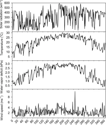
<1% of the time. Gaps were filled using linear interpolation for these short gaps by us- ing data between adjacent above and below gaps. The daily meteorological data were calculated using half an hour record and given in Fig. 1a (solar radiation, air temperature, water vapor pressure deficit (VPD) and wind speed measured at the 38 m height of the tower) and Fig. 1b (soil moisture, soil temperature at 5cm depth and precipita-

10

tion). The daytime was defined all half an hour records of solar radiation ≥10 w m⁻². There are 20–25 half an hour records for daytime in a day throughout a year. Dur- ing the observation period, the maximum daytime mean value of solar radiation was 591 w m⁻² (DOY 185) and annual mean air temperature during daytime was 21.0^◦C.

The maximum daytime mean value of VPD was 3.1 kPa (DOY 226) and yearly varia-

15

tions in the range 0.51–3.1 kPa. Wind speed was generally no more than 4 m s⁻¹ and an average annual value during daytime was 2.3 m s⁻¹.

3.2 Gap filling and CO fluxes data

To ensure data quality, CO₂ fluxes were edited manually to eliminate data due to obvious instrument failures or during rainfall when the open-path analyzer for CO₂ pro-

20

vides erroneous results. Satisfactory measurements were also obtained for CO₂fluxes throughout the year, with 658 bad records <8% of 8249 records in total. For conti- nuity of records, missing data for CO₂ fluxes were filled using relationships for CO₂ fluxes as a function of solar radiation, PAR, VPD and air temperature. We developed the procedure to maximize the correlations among these functions and found excel-

25

lent agreement using a simple regression analysis of CO₂ fluxes as a function of PAR

(9)

BGD

6, 2913–2937, 2009

Tables Figures

J I

Back Close

Full Screen / Esc

(Fig. 2). CO₂ fluxes were dependent mainly on variation of PAR, which was also in line with previous study (Rannik et al., 2002). Figure 2a compared half an hour CO₂ fluxes records during daytime with the corresponding PAR data from 8–26 January and R²=0.64 (n=352). We used this function to fill missing data for half hour records. The results were quite acceptable and a slight increase in R² (R²=0.69, n=356) was ob-

5

tained with a similar function of the mean PAR during daytime for the corresponding CO₂fluxes from the gap-filled data in 2003 (Fig. 2b).

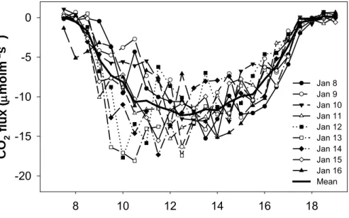
Half hourly records of CO₂ fluxes showed the typical fluctuations. Respective daytime CO₂fluxes between 8–16 January and their mean values are shown in Fig. 3. CO₂ was transported from air layer above the flux-measurement height to forest canopy and

10

the forest ecosystem was considered as a net sink of CO₂ during daytime. The maximum CO₂ uptake by forest occurred between 12:00 and 14:00, with a range of 15–

20 µmol m⁻²s⁻¹. The results were similar to previous studies in temperate deciduous broad-leaved forest and black spruce forest (Baldocchi and Vogel, 1996; Michael et al., 1997) and lower than a range of 18–27 µmol m⁻²s⁻¹ in boreal aspen forest (Black,

15

1996). The peaks of CO₂ fluxes appeared earlier than the peaks of solar radiation (Fig. 3). In such cases, the magnitude of CO₂fluxes increased rapidly in the morning, but decreased gradually in the afternoon (Fig. 3). The similar results were found in a Brazilian rain forest and a tropical rain forest at Pasoh in Peninsular Malaysia (Grace et al., 1996; Yasuda et al., 2003).

20

Using all daytime mean values in each month, we calculated the monthly values of CO₂fluxes, and applied them to further investigate seasonal variation in CO₂fluxes as shown in Fig. 4. CO₂ fluxes in the dry season (October to March) were slightly higher than those in the wet season (April to September). Contribution of CO₂ fluxes in the dry season was 53% of the annual total. The daytime CO₂ fluxes were very large in

25

October, November and December, which was therefore an important stage for uptake of CO₂by the forest ecosystem from the atmosphere.

Estimates of some model parameters were listed in Table 1. CBM also requires inputs of half an hour records of meteorological data including solar radiation, PAR, air

(10)

BGD

6, 2913–2937, 2009

Tables Figures

J I

Back Close

Full Screen / Esc

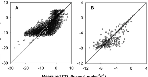
temperature, soil temperature, relative humidity, VPD, wind speed and rainfall. We used the gap-filled meteorological data at the top layer of tower for running a process-based model, CSIRO Biosphere Model (CBM). Figure 5a presented measured and modelled the daytime CO₂ fluxes of half an hour records during DOY 140–158. The results of model simulation sounded well on half an hour scale for daytime CO₂ fluxes, but un-

5

derestimated at noon and overestimated in the early morning and later afternoon. A comparison of the measured and simulated daytime CO₂ fluxes in 2003 was shown in Fig. 6a. The simulated daytime CO₂ fluxes with those of measured were relatively good (R²=0.63 n=8249). Only at high values the model tends to underestimate CO2

fluxes. The mean difference between the simulated and measured CO₂fluxes from the

10

year-round (8249 records) was −0.2 µmol m⁻²s⁻¹ and implied well within measurement accuracy. The model systematically overestimated the net CO₂ fluxes (i.e. the modelled net CO₂fluxes were more negative). The previous study suggested that the measured CO₂fluxes have random uncertainties from 10 to 20% because of stochastic natural turbulence (Rannik and Vesala, 1999).

15

Using half hourly records of the measured and simulated data, we calculated daytime mean values of CO₂ fluxes as shown in Fig. 5b. The mean daytime fluxes of the model performance in wet season were slightly higher than those of observations (see DOY 160–260), whereas for dry season, the CBM simulations were lower than those of measurements (see DOY 260–360). Although there was a relatively large scatter

20

on half hourly scale (Fig. 6a), the correlation coefficient between the measured and simulated data was high for the mean daytime CO₂ fluxes and significant (P <0.05 n=365). Plot of the model simulations versus the measured values of the mean daytime CO₂ fluxes is shown in Fig. 6b. The model explained more than 68% of the variation in the mean daytime CO₂fluxes in 2003.The monthly values of CO₂fluxes (measured

25

and modelled), PAR, based on the mean daytime values and rainfall monthly totals, are shown in Table 2.

(11)

BGD

6, 2913–2937, 2009

Tables Figures

J I

Back Close

Full Screen / Esc

4 Discussion

As stated in Table 2, both measured and modelled CO₂ fluxes showed that most of CO₂ uptake occurred during October–December, while least uptake occurred during February–March. In general, there is a strong positive correlation between CO₂ fluxes and PAR when PAR varies from zero to a potential maximum value (e.g.

5

2000 µmol m⁻²s⁻¹) that the whole ecosystem saturates (Kimball et al., 1997; Winner et al., 2004). Therefore, the observed low CO₂ uptake observed during February–

March could be attributed to lower PAR during this period, while a strong CO₂ uptake in October–December is attributed to high light intensities. The light-response of the whole ecosystem saturates at a light intensity of 600 to 800 µmol m⁻²s⁻¹

10

(Fig. 2b) and 1000 µmol m⁻²s⁻¹ (Fig. 2a) for the daytime mean values and the 30- min records, respectively, which is higher than the saturation photon flux density (400–

600 µmol m⁻²s⁻¹) of individual leaves of the dominant tree species in this forest (Sun, 1991). The peak of PAR occurred during July with a mean daily light intensity of 867 µmol m⁻²s⁻¹, which was higher than the saturation light intensity of the trees. This

15

could be one of reasons why the strong stage of CO₂ uptake was not directly related to the higher monthly PAR.

Rainfall events have significant effects on CO₂uptake by aggravating soil respiration and reducing plant photosynthesis (Davidson et al., 1998; Michael et al., 2002; Wright et al., 2005). Lots of rainfall events during the wet season could explain why this forest

20

ecosystem acted as a relative weak carbon sink. Based on PAR and rainfall, we could explain why the strong stage of CO₂ uptake did not coincide with the wet season, though, over which PAR and air temperature was high.

We calculated daytime uptake is only during the day C uptake of 957 gCm⁻²year⁻¹ and 991 gCm⁻²year⁻¹from measured and modelled results respectively. We however,

25

unable to estimate the net ecosystem exchange (NEE) directly due to uncertainties associated with measurements during the nighttime. Almost all eddy covariance limi- tations occur at night when the air becomes stably stratified. Some of these are instru-

(12)

BGD

6, 2913–2937, 2009

Tables Figures

J I

Back Close

Full Screen / Esc

mental; others are meteorological (Massman and Lee, 2002). In our measurements, we found obvious failure records were 3775>40% of 9271 in total. Soil respirations were measured in 2003/04 and released 1001 gCm⁻²year⁻¹ in this forest stand (Yan et al., 2006). Soil respirations were also relatively constant on a diurnal time scale because changes in soil moisture are very slow and there is no significant relation

5

between soil moisture and temperature, which tend to behave erratically, so that their effects may tend to cancel each other (Yan et al., 2006). Therefore, we can assume soil respirations during nighttime was 501 gCm⁻²year⁻¹(a half of 1001 gCm⁻²year⁻¹).

Soil respirations were 65–80% of ecosystem respirations generally (Wang et al., 2004).

The NEE was estimated −242 and −276 gCm⁻²year⁻¹ for measured and modelled,

10

respectively, according to soil respirations accounting for 70% of ecosystem respirations (715 gCm⁻²year⁻¹, C released during nighttime was 712 gCm⁻²year⁻¹based on CBM outputs. Our results show higher rates of CO₂ fluxes than the range of −133 to −254 gCm⁻²year⁻¹ reported by Wang et al. (2004) for a pine forest and similar to NEE for a southern boreal aspen forest reported by Griffis et al. (2004). Fan et

15

al. (1990) and Grace et al. (1996) evaluated the daily values of NEE in Amazonian tropical forests as about −0.60 gCm⁻² per day calculated from a short-term measurement and −0.54 gCm⁻² per day measured during a 44-day-observation. Moreover, Grace et al. (1996) and Yasuda (2003) obtained daily NEE in the Amazonian forest in the dry season as −1.08 gCm⁻²per day and −2.44 gCm⁻²per day in a tropical rain

20

forest based on 7-day-measurement. NEE in this study was similar to the median value of the range reported in previous findings, although most of data originate from short- term estimates. The NPP for this forest stand was 694 gCm⁻²year⁻¹ during 2003/04 estimated by Yan et al. (2006) and the litter fall was 424 gCm⁻²year⁻¹. We therefore calculated the NEE was 270 gCm⁻²year⁻¹ and very similar to the values obtained by

25

CO₂ fluxes measured and modelled in this study. CBM sensitivity analysis has been executed in previous studies (Wang and Leuning, 1998; Wang, 2000; Wang et al., 2001). In this study, it was difficult to make a statistically accurate determination of the optimal parameter combinations. The two key parameters canopy leaf area index (L)

(13)

BGD

6, 2913–2937, 2009

Tables Figures

J I

Back Close

Full Screen / Esc

and maximum carboxylation rate (v_cmax) were constant throughout because of the high temperature and evergreen nature of the forest ecosystem. By tuning on these two key parameters in the model, L (Range 4.5–8.0) and v_cmax (18–28), no better results were obtained. We suspected that this behavior was likely to be the result of CBM using constant vegetation parameters and fitted very well to simulate CO₂ fluxes for

5

evergreen forests in the tropical and subtropical regions.

Acknowledgements. We thank Mr. Meng Ze and Mr. Mo Dingsheng for their fieldwork during data collection. Also, we are grateful to Wang Xu and, Wang Chunlin for their hard work in the laboratory during measurement. This study was supported by grants from the Natural Science Foundation of China (30590381-03), project of international foundation of science (D/3491-1)

10

and key knowledge innovation funding from the Chinese Academy of Sciences (KZCX1-SW- 01).

References

Baadocchi, D. D. and Vogel, C. A.: Energy and CO₂flux densities above and below a temperate broad-leaved forest and a boreal pine forest, Tree Physiol., 16, 5–16, 1996.

15

Black, T. A., Denhartog, G., Neumann, H. H., et al.: Annual cycles of water vapor and carbon dioxide fluxes in and above a boreal aspen forest, Glob. Change Biol., 102, 219–229, 1996.

Cao, M. K., Tao, B., Li, K. R., Shao, X. M., and Stephen, D. P.: Interannual variation in terrestrial ecosystem carbon Fluxes in China from 1981 to 1998, Acta Bot. Sin., 45(5), 552–560, 2003.

Clapp, R. B. and Hornberger, M. G.: Empirical equations for some soil hydraulic properties,

20

Water Resour. Res., 14, 601–604, 1978.

Davidson, E. A., Belk, E., and Boone, R. D.: Soil water content and temperature as independent or confounded factors controlling soil respiration in a temperate mixed hardwood forest, Glob.

Change Biol., 4, 217–222, 1998.

Dennis, D. B., Bruce, B. H., and Tilden, P. M.: Measuring biosphere-atmosphere exchange

25

of biologically related gases with micrometeorological methods, Ecology, 69(5), 1331–1340, 1988.

Edwards, N. T. and Sollins, P.: Continuous measurement of carbon dioxide evolution from partitioned forest floor components, Ecology, 54, 406–412, 1973.

(14)

BGD

6, 2913–2937, 2009

Tables Figures

J I

Back Close

Full Screen / Esc

Fan, S.-M., Wofsy, S. C., Bakwin, P. S., and Jacob, D. J.: Atmosphere-biosphere exchange of CO₂and O₃in the Central Amazon forest, J. Geophys. Res., 95(D10), 16851–16864, 1990.

Fang, J. Y., Chen, A. P., Peng, C. H., Zhao, S. Q., and Ci, L. J.: Changes in forest biomass carbon storage in China between 1949 and 1998, Science, 292, 2320–2322, 2001.

Fang, J. Y. and Chen, A. P.: Dynamic forest biomass carbon pools in China and their signifi-

5

cance, Acta Bot. Sin., 43(9), 967–973, 2001 (in Chinese).

GCN FLUXNET: CO₂flux monitoring network, Glob. Change Newslett., 22, 7–8, 1995.

Grace, J., Malhi, Y., Lloyd, J., Mclntyre, J., Miranda, A. C., Meir, P., and Miranda, H. S.: The use of eddy covariance to infer the net carbon dioxide dioxide uptake by Brazilian rain forest, Glob. Change Biol., 2, 209–218, 1996.

10

Griffis, T. J., Black, T. A., Guay, D. G., et al.: Seasonal variation and partitioning of ecosystem respiration in a southern boreal aspen forest, Agr. Forest Meteorol., 125, 207–223, 2004.

Huang, Z. L., Ding, M. M., Zhang, Z. P., and Yi, W. M.: The hydrological processes and nitrogen dynamics in a monsoon evergreen broad-leafed forest of Dinghushan. Acta Phytoecology Sinica, 18(2), 194–199, 1994.

15

Keller, M., Kaplan, W. A., Wofsy, S. C.: Emissions of N₂O, CH₄and CO₂from tropic forest soils, J. Geophys. Res., 91, 11791–11802, 1986.

Kimball, J. S., Thornton, P. E., White, M. A., and Running, S. W.: Simulating forest productivity and surface-atmosphere carbon exchange in the BOREAS study region, Tree Physiol., 17, 589–599, 1997.

20

Kowalczyk, E. A., Garratt, J. R., and Krummel, P. B.: Implementation of a soil-canopy scheme into the CSIRO GCM – regional aspects of the model response, CSIRO Division of Atmo- spheric Research technical paper, No. 32, Melbourne, Australia, 59 pp., 1994.

Massman, W. J and Li, X.: Edd covariance flux corrections and uncertainties in long-term studies of carbon and energy exchanges, Agr. Forest Meteorol., 113, 121–144, 2002.

25

Michael, F. L., Duchesne, L. C., and Wetzel, S.: Effect of rainfall patterns on soil surface CO₂ efflux, soil moisture, soil temperature and plant growth in a grassland ecosystem of northern Ontario, Canada: implications for climate change, BMC Ecology, 2(10), 1–6, 2002.

Michael, L. G., Bruce, C. D., Fan, S. M., et al.: Physiological responses of a black spruce forest to weather, J. Geophys. Res., 102, 28987–28996, 1997.

30

Mo, J. M., Brown, S., Ding, M. M., Zhang, Z. P.: Nitrogen distribution in vegetation of a subtropical monsoon evergreen broadleaf forest in China, Tropics, 3(2), 143–153, 1994.

Peng, S. L. and Zhang, Z. P.: Biomass, productivity and energy use efficiency of climax vege-

(15)

BGD

6, 2913–2937, 2009

Tables Figures

J I

Back Close

Full Screen / Esc

tation on Dinghu Mountains, Guangdong, China, Sci. China Ser. B, 38(1), 67–73, 1995.

Rannik, U., Altimir, N., Raittila, J., et al.: Fluxes of carbon dioxide and water vapour over Scots pine forest and clearing, Agr. Forest Meteorol., 111, 187–202, 2002.

Rannik, U. and Vesala, T.: Autoregressive filtering versus linear detrending in estimation of fluxes by the eddy covariance method, Bound.-Lay. Meteorol., 91, 259–280, 1999.

5

Sellers, P. J., Tucker, C. J., Collatz, G. J., Los, S. O., Justice, C. O., Dazlich, D. A., and Randall, D. A.: A global1 degrees-by-1 degrees NDVI data set for climate studies. 2. The generation of global fields of terrestrial biophysical parameters from the NDVI, Int. J. Remote Sens., 15, 3519–3545, 1994.

Sun, G. C.: Comparative photosynthesis of plants grown in various site of subtropical monsoon

10

broad-leaved forest, Guihaia, 11(1), 51–57, 1991.

Tang, X. L., Liu, S. G., Zhou, G. Y., Zhang, D. Q., and Zhou, C. Y.: Soil-atmospheric exchange of CO₂, CH₄, and N₂O in three subtropical forest ecosystems in southern China, Glob. Change Biol., 12, 546–560, 2006.

Tang, X. L., Zhou, G. Y., and Liu, S. G., et al.: Woody debris biomass and its potential contri-

15

bution to carbon cycle in successional subtropical forests of Southern China, Acta Phytoe- cologica Sinica, 29, 559–568, 2005.

Wang, K. Y., Kellomaki, S., Zha, T. S., and Peltola, H.: Component carbon fluxes and their contribution to ecosystem carbon exchange in a pine forest: an assessment based on eddy covariance measurements and an integrated model, Tree Physiol., 24, 19–34, 2004.

20

Wang, Y. P.: An improvement to the two-big-leaf model for calculating canopy photosynthesis, Agr. Forest Meteorol., 10, 143–150, 2000.

Wang, Y. P. and Leuning, R.: A two-leaf model for canopy conductance, photosynthesis and partitioning of available energy I. model description and comparison with a multi-layered model, Agr. Forest Meteorol., 91, 89–111, 1998.

25

Wang, Y. P., Leuning, R., Cleugh, H. A., and Coppin, P. A.: Parameter estimation in surface exchange models using nonlinear inversion: how many parameters can we estimate and which measurements are most useful?, Glob. Change Biol., 7, 495–510, 2001.

Wang, X. K., Feng, Z. Y., and Ouyang, Z. Y.: The impact of human disturbance on vegetative carbon storage in forest ecosystems in China, Forest Ecol. Manage., 148, 117–123, 2001.

30

Winner, W. E., Thomas, S. C., Berry, J. A., et al.: Canopy carbon gain and water use: Analysis of old-growth confers in the Pacific Northwest, Ecosystem, 7, 482–497, 2004.

Wright, I. J., Reich, P. B., Atkin, O. K., Lusk, C. H., Tjoelker, M. J., and Westoby, M.: Ir-

(16)

BGD

6, 2913–2937, 2009

Tables Figures

J I

Back Close

Full Screen / Esc

radiance, temperature and rainfall influence leaf dark respiration in woody plants: evi- dence from comparisons across 20 sites, New Phytol., 169, 309–319, doi:10.1111/j.1469- 8137.2005.01590.x, 2006.

Yan, J. H., Wang, Y. P., Zhou, G. Y., and Zhang, D. Q.: Estimates of soil respiration and net pri- mary production of three forests at different succession stages in South China, Glob. Change

5

Biol., 12, 810–821, 2006.

Yan, J. H., Zhou, G. Y., and Chen, Z. Y.: Coupling study on soil structure and hydrological effects for three succession communities in Dinghushan. Development of Research Network for Natural Resources, Environ. Ecol., 11(1), 6–11, 2000.

Yasuda, Y., Ohtani, Y., Watanabe, T., et al.: Measurement of CO₂ flux above a tropical rain

10

forest at Pasoh in Peninsular Malaysia, Agr. Forest Meteorol., 114, 235–244, 2003.

Yi, Z. G., Yi, W. M., Zhou, G. Y., Ding, M. M., and Zhou, L. X.: Soil carbon effluxes of three major vegetation types in Dinghushan Biosphere Reserve, Acta Ecologica Sinica, 23, 1673–1678, 2003.

Zhang, B. G. and Zhuo, M. N.: The physical properties of soil under different forest types in

15

Dinghushan Biosphere Reserve, Tropical and Subtropical Forest Ecosystem, 3, 1–9, 1985.

Zhou, C. Y., Zhou, G. Y., Zhang, D. Q., et al.: CO₂efflux from different forest soils and impact factors in Dinghu Mountain, China, Sci. Ser. D, 34 (supplement), 175–182, 2004.

Zhou, G. Y., Jim, M., Zhou, C. Y., Yan, J. H., and Huang, Z. L.: Hydrological processes and vegetation succession in a naturally forested area of southern China, Eurasian Journal of

20

Forest Research, 7(2), 75–86, 2004.

Zhou, G. Y. and Yan, J. H.: The influences of regional atmospheric precipitation characteristics and its element inputs on the existence and development of Dinghushan forest ecosystems, Acta Ecology Sinica, 21(12), 2002–2012, 2001.

Zhou, G. Y., Zhou, C. Y., Liu, S. G., et al.: Belowground carbon balance and carbon accumu-

25

lation rate in the successional series of monsoon evergreen broad-leaved forest, Sci. China Ser D, 49(3), 311–321, 2006.

(17)

BGD

6, 2913–2937, 2009

Tables Figures

J I

Back Close

Full Screen / Esc

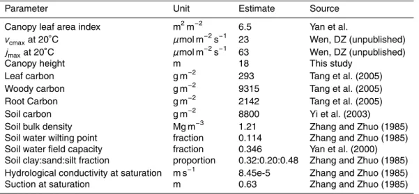
Table 1. Estimates of vegetation and soil properties from past studies at Dinghushan Station.

Parameter Unit Estimate Source

Canopy leaf area index m²m⁻² 6.5 Yan et al.

v_cmaxat 20^◦C µmol m⁻²s⁻¹ 23 Wen, DZ (unpublished)

j_maxat 20^◦C µmol m⁻²s⁻¹ 63 Wen, DZ (unpublished)

Canopy height m 18 This study

Leaf carbon g m⁻² 293 Tang et al. (2005)

Woody carbon g m⁻² 9315 Tang et al. (2005)

Root Carbon g m⁻² 2142 Tang et al. (2005)

Soil carbon g m⁻² 8800 Yi et al. (2003)

Soil bulk density Mg m⁻³ 1.21 Zhang and Zhuo (1985)

Soil water wilting point fraction 0.114 Zhang and Zhuo (1985) Soil water field capacity fraction 0.346 Yan et al. (2000) Soil clay:sand:silt fraction proportion 0.32:0.20:0.48 Zhang and Zhuo (1985) Hydrological conductivity at saturation m s⁻¹ 8.45e-5 Zhang and Zhuo (1985)

Suction at saturation m 0.63 Zhang and Zhuo (1985)

(18)

BGD

6, 2913–2937, 2009

Tables Figures

J I

Back Close

Full Screen / Esc

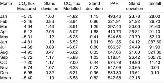
Table 2. Monthly averages for daytime CO₂fluxes (measured and modelled) and PAR. Rainfall was calculated the total during 24-h in each month.

Month CO₂flux Stand CO₂flux Stand PAR Stand rainfall Measured deviation Modelled deviation deviation

Jan −5.75 1.60 −4.82 1.13 493.46 23.78 28.00

Feb −3.46 0.83 −3.94 0.96 321.91 21.92 26.70

Mar −4.04 1.43 −3.91 1.29 297.40 20.00 91.60

Apr −5.12 2.05 −5.07 1.68 413.73 25.81 91.10

May −5.31 1.12 −6.25 0.41 544.66 23.79 52.10

Jan −4.81 1.19 −5.52 1.01 501.35 24.12 287.60

Jul −4.68 0.83 −6.07 0.80 866.57 24.49 91.90

Aug −4.93 0.47 −6.02 0.35 647.66 21.60 321.80

Sep −5.72 1.17 −5.88 1.03 618.51 26.42 305.70

Oct −7.20 1.17 −7.00 0.44 674.78 19.90 11.40

Nov −6.74 1.07 −6.23 0.73 547.09 20.65 0.00

Dec −6.98 0.32 −6.31 0.96 583.80 13.61 0.10

Mean −5.40 1.10 −5.58 0.82 542.58 22.18 –

(19)

BGD

6, 2913–2937, 2009

Tables Figures

J I

Back Close

Full Screen / Esc

Printer-friendly Version Interactive Discussion Day of year, 2003

0 20 40 60 80100 120

140 160

180 200

220 240

260 280

300 320

340 360 Wind speed (ms-1)

2 4 6 8 Water vapor deficit (kPa) 10

0.5 1.0 1.5 2.0 2.5 3.0 Temperature (0C)

5 10 15 20 25 30 Solar radiation (wm-2)

100 200 300 400 500 600

182

Fig. 1a.

Fig. 1a. Variations of daytime mean values in solar radiation, air temperature, VPD (water183 vapor deficit) and wind speed at 38 m height in 2003.

2931

(20)

BGD

6, 2913–2937, 2009

Tables Figures

J I

Back Close

Full Screen / Esc

Soil Temperature (¡æ)

5 10 15 20 25 30 Tsoil

Soil Moisture (m3 m-3 ) .10 .15 .20 .25 .30 .35

DOY

0 60 120 180 240 300 360

Precipitation (mm)

0 20 40 60 80 100

Precipitation

184

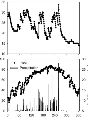
Fig.1b.

185 186

Photon flux density (μmolm^-2s^-1)

0 200 400 600 800 1000 1200 1400

CO2 flux (μmolm-2 s-1 )

-25 -20 -15 -10 -5 0

0 200 400 600 800 1000 1200 1400 -25

-20 -15 -10 -5

0 B

A

187

Fig. 2.

188

Fig. 1b. Variations of daily mean soil moisture, soil temperature at 5cm depth and daily precip- itation.

2932

(21)

BGD

6, 2913–2937, 2009

Tables Figures

J I

Back Close

Full Screen / Esc

Printer-friendly Version Interactive Discussion 22

Soil Temperature (¡æ)

5 10 15 20 25 30 Tsoil

Soil Moisture (m3 m-3 ) .10 .15 .20 .25 .30 .35

DOY

0 60 120 180 240 300 360

Precipitation (mm)

0 20 40 60 80 100

Precipitation

184

Fig.1b.

185 186

Photon flux density (μmolm^-2s^-1)

0 200 400 600 800 1000 1200 1400

CO2 flux (μmolm-2 s-1 )

-25 -20 -15 -10 -5 0

0 200 400 600 800 1000 1200 1400 -25

-20 -15 -10 -5

0 B

A

187

Fig. 2.

188 Fig. 2. Response of daytime CO₂fluxes to photon flux density.(A) was half-hour records during daytime with the corresponding photon flux density data from 8–26 January;(B) was the mean daytime CO₂fluxes with the corresponding photon flux density data in 2003.

(22)

BGD

6, 2913–2937, 2009

Tables Figures

J I

Back Close

Full Screen / Esc

Time of day (h)

8 10 12 14 16 18

CO 2 flux (μmolm-2 s-1 ) -20 -15 -10 -5 0

Jan 8 Jan 9 Jan 10 Jan 11 Jan 12 Jan 13 Jan 14 Jan 15 Jan 16 Mean

189

Fig. 3.

190

191

Jan Feb Mar Apr May Jun Jul Aug Sep Oct Nov Dec

CO2 flux (μmolm-2 s-1 ) -10

-8 -6 -4 -2 0

192

Fig. 4.

193

194

195

196

Fig. 3. Variations in half an hour records of CO₂fluxes during daytime on 8–16 January and their mean values with the dashed line.

2934

(23)

BGD

6, 2913–2937, 2009

Tables Figures

J I

Back Close

Full Screen / Esc

23

Time of day (h)

8 10 12 14 16 18

CO 2 flux ( μmo lm -2 s -1 )

-20 -15 -10 -5 0

Jan 8 Jan 9 Jan 10 Jan 11 Jan 12 Jan 13 Jan 14 Jan 15 Jan 16 Mean

189 Fig. 3.

190 191

Jan Feb Ma r Apr Ma y Jun Jul Aug Sep Oc t Nov Dec

CO

2

fl ux ( μmol m

-2

s

-1

) -10

-8 -6 -4 -2 0

192 Fig. 4.

193 194 195

196

Fig. 4. Variations in eddy covariance measurements of monthly CO₂fluxes and their SD.

2935

中国生态系统研究网络

BGD

A comparison of CO 2 fluxes via eddy covariance measurements with model predictions in a dominant subtropical forest ecosystem

BGD

BGD

BGD

BGD

BGD

BGD

BGD

BGD

BGD

BGD

BGD

BGD

BGD

BGD

BGD

BGD

BGD

BGD

BGD

BGD

BGD

BGD

23

Time of day (h)

8 10 12 14 16 18

CO 2 flux ( μmo lm -2 s -1 )

-20 -15 -10 -5 0

Jan 8 Jan 9 Jan 10 Jan 11 Jan 12 Jan 13 Jan 14 Jan 15 Jan 16 Mean

189

Fig. 3.

190 191

Jan Feb Ma r Apr Ma y Jun Jul Aug Sep Oc t Nov Dec

CO

fl ux ( μmol m

s

) -10

-8 -6 -4 -2 0

192

Fig. 4.

193 194 195

196

A comparison of CO ₂ fluxes via eddy covariance measurements with model predictions in a dominant subtropical forest ecosystem