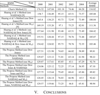
A new method to forecast the TAIEX based on fuzzy time series

A New Method to Forecast the TAIEX Based on Fuzzy Time Series

Chao-Dian Chen ¹ and Shyi-Ming Chen ^{1, 2}

1 Department of Computer Science and Information Engineering, National Taiwan University of Science and Technology, Taipei, Taiwan, R. O. C.

2 Department of Computer Science and Information Engineering, Jinwen University of Science and Technology, Taipei County, Taiwan, R. O. C.

Abstract—In this paper, we present a new method to forecast the Taiwan Stock Exchange Capitalization Weighted Stock Index (TAIEX) based on fuzzy time series, where the main factor is the TAIEX and the secondary factors are either the Dow Jones, the NASDAQ, the M 1b (Taiwan), or their combinations. First, we fuzzify the historical data of the main factor into fuzzy sets with a fixed length of intervals to form fuzzy logical relationships. Then, we group the fuzzy logical relationships into fuzzy logical relationship groups. Then, we evaluate the leverage of fuzzy variations between the main factor and the secondary factor to forecast the TAIEX. The experimental results show that the proposed method gets a higher average forecasting accuracy rate than Chen’s method [1] and Huarng et al.’s method [9] to forecast the TAIEX.

Keywords—fuzzy sets, fuzzy time series, fuzzy logical relationships, fuzzy variation

I. I NTRODUCTION

In [11], [12] and [13], Song and Chissom presented the concepts of fuzzy time series based on the fuzzy set theory [21], where the values of a fuzzy time series are represented by fuzzy sets. In recent years, some methods have been presented to handle forecasting problems based on fuzzy time series, such as enrollments forecasting [1], [2], [3], [4], [12], [13], [15], [19], temperature prediction [5], [10], [14], stock index forecasting [6], [7], [8], [9], [14], [16], [17], [18], [20] , …, etc.

In this paper, we present a new method to forecast the Taiwan Stock Exchange Capitalization Weighted Stock Index (TAIEX) based on fuzzy time series, where the main factor is the TAIEX and the secondary factors are either the Dow Jones, the NASDAQ, the M 1b (Taiwan), or their combinations. First, we fuzzify the historical data of the main factor into fuzzy sets with a fixed length of intervals to form fuzzy logical relationships. Then, we group the fuzzy logical relationships into “fuzzy logical relationships groups”. Then, we evaluate the leverage of fuzzy variations between the main factor and the secondary factor to forecast the TAIEX. The experimental results show that the proposed method gets a higher average forecasting accuracy rate than Chen’s method [1] and Huarng et al.’s method [9] to forecast the TAIEX.

The rest of this paper is organized as follows. In Section II, we briefly review the definition of fuzzy time series from [11], [12] and [13]. In Section III, we present a new method based on fuzzy time series to forecast the TAIEX. In Section IV, we make a comparison of the experimental results of the proposed method with the existing methods. The conclusions are discussed in Section V.

II. P RELIMINARIES

In [11], [12] and [13], Song and Chissom presented the concepts of fuzzy time series based on the fuzzy set theory [21], where the values of a fuzzy time series are represented by fuzzy sets. Let U be the universe of discourse, where U = {u 1 , u 2 , …, u n }. A fuzzy set A i in the universe of discourse U is defined as follows:

A i = f Ai (u 1 )/u 1 + f Ai (u 2 )/u 2 + …+ f Ai (u n )/u n ,

where f _Ai is the membership function of the fuzzy set A _i , f _Ai (u _j ) is the degree of membership of u _j belonging to the fuzzy set A _i , f Ai (u j ) ∈[0,1] and 1 ≤ j ≤ n.

Definition 2.1 [11]: Let Y(t) (t = …, 0, 1, 2, …) be the universe of discourse and be a subset of R. Assume that f i (t) (i = 1, 2, …) are defined in the universe of discourse Y(t), and assume that F(t) is a collection of f i (t) (i = 1, 2, …), then F(t) is called a fuzzy time series of Y(t) (t = …, 0, 1, 2, …).

If a fuzzy relationships R(t −1,t) exists, such that F(t) = F(t −1) D R(t−1,t), where the symbol “D” represents the max −min composition operator, then F(t) is called caused by F(t −1) [11].

Definition 2.2 [11]: Let F(t−1) = A i and let F(t) = A ^j . The relationship between F(t −1) and F(t) can be denoted by fuzzy logical relationship A i → A j , where A i is called the left-hand side (LHS) and A j is called the right-hand side (RHS) of the fuzzy logical relationship.

Fuzzy logical relationships having the same left-hand side can be grouped into a fuzzy logical relationship group (FLRG) [1]. For example, assume that the following fuzzy logical relationships exist:

A i → A ^ja , A i → A ^jb ,

#

A _i → A jm .

then these fuzzy logical relationships can be grouped into a fuzzy logical relationship group, shown as follows:

A i → A ja , A jb , …, A jm .

III. A N EW M ETHOD FOR F ORECASTING THE TAIEX B ASED ON F UZZY T IME S ERIES

In this section, we present a new method to forecast the TAIEX from 2000 to 2004 based on fuzzy time series, where Proceedings of the 2009 IEEE International Conference on Systems, Man, and Cybernetics

San Antonio, TX, USA - October 2009

the historical data are divided into two parts, i.e., the training data set and the testing data set. The training data set consists of the historical data from January to October for each year, and the testing data set consists of the historical data from November to December for each year. Table I [9] shows the TAIEX, the Dow Jones, the NASDAQ, and the M _1b from January 2004 to December 2004. In this paper, the TAIEX is the main factor, where the secondary factors Dow Jones, NASDAQʳ and M 1b are used to forecast the TAIEX. The proposed method is now presented as follows:

Step 1: Define the universe of discourse U, U = [D min −D 1 , D _max +D ₂ ], where D _min and D _max are the minimum and the maximum values of the historical data of the main factor, respectively; D ₁ and D ₂ are two proper positive real values to partition the universe of discourse U into n intervals u ₁ , u ₂ , …, and u _n of equal length. For example, from Table I, we can see that the minimum and the maximum values of the training data of the TAIEX of the year 2004 are 5316.87 and 7034.1, respectively. If we let D ₁ = 16.87 and D 2 = 65.9, then the universe of discourse U = [5300, 7100]. Let the length of each interval in the universe of discourse U be 100. Then, the universe of discourse U can be divided into 18 intervals, which is defined as follows:

u i = [5300 + (i − 1) × 100, 5300 + (i) × 100], (1) where i = 1, 2, …, 18.

TABLE I. H ISTORICAL D ATA OF THE TAIEX, THE D OW J ONES , THE

NASDAQ, AND THE M1 B OF 2004 [9]

Date TAIEX Dow Jones NASDAQ M

1b

2004/1/2 6041.56 10409.85 2006.68 6491205 2004/1/5 6125.42 10544.07 2047.36 6487349 2004/1/6 6144.01 10538.66 2057.37 6497906

# # # # #

2004/11/1 5656.17 10054.39 1979.87 7040767 2004/11/2 5759.61 10035.73 1984.79 7054955

# # # # #

2004/12/31 6139.69 10783.01 2175.44 7370450

Step 2: Define the linguistic terms A i represented by fuzzy sets, shown as follows:

A 1 = 1/u 1 + 0.5/u 2 + 0/u 3 + … + 0/u n −2 + 0/u n −1 + 0/u n , A 2 = 0.5/u 1 + 1/u 2 + 0.5/u 3 + … + 0/u n −2 + 0/u n −1 + 0/u n ,

#

A _n = 0/u 1 + 0/u ₂ + 0/u ₃ + … + 0/u _n−2 + 0.5/u _n−1 + 1/u _n . where A ₁ , A ₂ , …, and A _n are linguistic terms. For example, based on the obtained 18 intervals, we can define the linguistic terms A ₁ , A ₂ , …, and A ₁₈ , shown as follows:

A ₁ = 1/u 1 + 0.5/u ₂ + 0/u ₃ + … + 0/u ₁₆ + 0/u ₁₇ + 0/u ₁₈ , A ₂ = 0.5/u 1 + 1/u ₂ + 0.5/u ₃ + … + 0/u ₁₆ + 0/u ₁₇ + 0/u ₁₈ ,

#

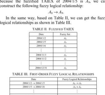
A 18 = 0/u 1 + 0/u 2 + 0/u 3 + … + 0/u 16 + 0.5/u 17 + 1/u 18 . Step 3: Fuzzify each historical datum of the main factor into a fuzzy set defined in Step 2. If the historical datum of the main factor belongs to u i and the maximum membership value of the fuzzy set A i occurs at u i , where 1 ≤ i ≤ n, then the historical datum of the main factor is fuzzified into A i . For example, from Table I, we can see that the TAIEX of 2004/1/2 is 6041.56, which can be fuzzified into A 8 . Table II shows the fuzzified TAIEX of the data shown in Table I, respectively.

Step 4: Construct fuzzy logical relationships from the fuzzified historical data of the main factor obtained in Step 3. For example, from the fuzzified TAIEX of the training data shown in Table II, we can construct fuzzy logical relationships. For example, because the fuzzified TAIEX of 2004/1/2 is A ₈ and because the fuzzified TAIEX of 2004/1/5 is A ₉ , we can construct the following fuzzy logical relationship:

A ₈ → A 9 .

In the same way, based on Table II, we can get the fuzzy logical relationships as shown in Table III.

TABLE II. F UZZIFIED TAIEX

Date Fuzzy Set

2004/1/2 A

8

2004/1/5 A

9

2004/1/6 A

9

# #

2004/11/1 A

4

2004/11/2 A

5

# #

2004/12/31 A

9

TABLE III. F IRST -O RDER F UZZY L OGICAL R ELATIONSHIPS Date Fuzzy Logical Relationships 2004/1/2 → 2004/1/5 A

8

→ A

9

2004/1/5 → 2004/1/6 A

9

→ A

9

# #

2004/10/28 → 2004/10/29 A

4

→ A

5

Step 5: Fuzzify the variation between the adjacent historical data of the main factor and the secondary factors, respectively, and then group the fuzzy logical relationships of the main factor. The sub-steps are shown as follows:

Step 5.1: Calculate the variation of the close index between the adjacent historical data, where the variation Var t on day t is calculated as follows:

Close % Close Close Var

t t t

t

100

1 1

×

= −

−

−

, (2)

where the terms Close t and Close t −1 are the close indices on the trading day t and trading day t −1, respectively, and the unit of the variation is the percentage. For example, from Table I, we can see that the TAIEX of 2004/1/2 and 2004/1/5 are 6041.56 and 6125.42, respectively. Based on Eq. (2), we can see that the variation of the TAIEX on 2004/1/5 is equal to

. % .

. 100

56 6041

56 6041 42

6125 − × = 1.388052 %. Table IV and Table V show the variation of the TAIEX, the Dow Jones, the NASDAQ and the M 1b of the training data and the testing data.

TABLE IV. T HE V ARIATION OF THE T RAINING D ATA OF TAIEX, THE

D OW J ONES , THE NASDAQ, AND THE M

1B

(U NIT : %)

Date Variation of the TAIEX

Variation of the Dow Jones

Variation of the NASDAQ

Variation of the M

1b

2004/1/5 1.388052 % 1.289356 % 2.027229 % -0.059403 % 2004/1/6 0.303489 % -0.051308 % 0.488922 % 0.162732 %

# # # # #

2004/10/29 0.182072 % 0.229196 % -0.037960 % 0.639198 %

TABLE V. T HE V ARIATION OF THE T ESTING D ATA OF TAIEX, THE D OW J ONES , THE NASDAQ AND THE M

1B

(U NIT : %)

Date Variation of the TAIEX

Variation of the Dow Jones

Variation of the NASDAQ

Variation of the M

_1b

2004/11/1 -0.872075 % 0.268463 % 0.247090 % -0.348530 % 2004/11/2 1.828799 % -0.185591 % 0.248501 % 0.201512 %

# # # # #

2004/12/30 0.203170 % -0.266779 % 0.061553 % 0.979241 %

Step 5.2: Define the universe of discourse V, V = [E min , E _max ], where E _min and E _max are the minimum and the maximum variation of the main factor and secondary factors, respectively.

It should be noted that the minimum and the maximum limited variations of the TAIEX are -7% and 7%, respectively, and the minimum and the maximum limited variations of the Dow Jones, the NASDAQ and the M _1b are not limited, respectively.

The universe of discourse V is defined as [- ∞, ∞]. We let the length of each interval between -6% and 6% be equal to 1.

Then, the universe of discourse V can be divided into 14 intervals v 1 , v 2 , …, and v 14 , where v 1 = [-∞, -6], v 2 = [-6, -5], …, and v 14 = [6, ∞], as shown in Table VI.

TABLE VI. 14 I NTERVALS IN THE U NIVERSE OF D ISCOURSE V (U NIT : %)

v

1

= [-∞, -6] v

4

= [-4, -3] v

7

= [-1, 0] v

10

= [2, 3] v

13

= [5, 6]

v

2

= [-6, -5] v

5

= [-3, -2] v

8

= [0, 1] v

11

= [3, 4] v

14

= [6, ∞]

v

3

= [-5, -4] v

6

= [-2, -1] v

9

= [1, 2] v

12

= [4, 5]

Step 5.3: Define the linguistic term B j represented by fuzzy sets, shown as follows:

B 1 = 1/v 1 + 0.5/v 2 + 0/v 3 +…+ 0/v m −2 + 0/v m −1 + 0/v m , B 2 = 0.5/v ¹ + 1/v 2 + 0.5/v 3 +…+ 0/v m −2 + 0/v m −1 + 0/v m ,

#

B m = 0/v 1 + 0/v 2 + 0/v 3 +…+ 0/v m −2 + 0.5/v m −1 + 1/v m . where B ₁ , B ₂ , …, and B _m are linguistic terms. For example, based on Table VI, we can define the linguistic terms B ₁ , B ₂ ,

…, and B ₁₄ , shown as follows:

B ₁ = 1/v 1 + 0.5/v ₂ + 0/v ₃ +…+ 0/v ₁₂ + 0/v ₁₃ + 0/v ₁₄ , B ₂ = 0.5/v 1 + 1/v ₂ + 0.5/v ₃ +…+ 0/v ₁₂ + 0/v ₁₃ + 0/v ₁₄ ,

#

B ₁₄ = 0/v 1 + 0/v ₂ + 0/v ₃ +…+ 0/v ₁₂ + 0.5/v ₁₃ + 1/v ₁₄ .

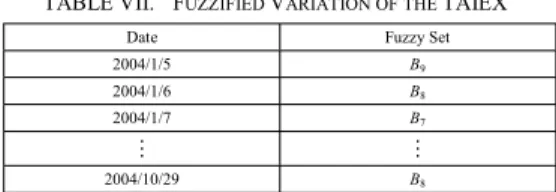
Step 5.4: Fuzzify each historical variation of the main factor into a fuzzy set defined in Step 5.2. If the historical variation of the main factor on day t belongs to v _j , where 1 ≤ j ≤ m, then the historical variation of the main factor on day t is fuzzified into B _j . For example, from Table IV, we can see that the variation of the TAIEX on 2004/1/5 is 1.388052%, which is fuzzified into B ₉ . Table VII shows the fuzzified variation of the TAIEX of the training data.

TABLE VII. F UZZIFIED V ARIATION OF THE TAIEX

Date Fuzzy Set

2004/1/5 B

9

2004/1/6 B

8

2004/1/7 B

7

# #

2004/10/29 B

8

Step 5.5: Based on the linguistic terms of the fuzzified variations, group the fuzzy logical relationships having the same linguistic term of the fuzzified variation into a fuzzy logical relationship group. For example, let us consider the following fuzzy logical relationships: “A a1 → A aa ”, where the fuzzified variation is B z ; “A a1 → A ab ”, where the fuzzified variation is B z ; “A a1 → A ac ”, where the fuzzified variation is B _z ; …; “A a1 → A ak ”, where the fuzzified variation is B z . Then, these fuzzy logical relationships can be grouped into the same fuzzy logical relationship group in which the fuzzified variation

of each fuzzy logical relationship in this group is B _z , shown as follows:

A _a1 → A aa , A _ab , A _ac , …, A _ak .

For example, from Table III, we can see that the fuzzy logical relationship between the trading days 2004/1/2 and 2004/1/5 is A ₈ → A 9 , from Table VII, we can see that the fuzzified variation on 2004/1/5 is B ₉ ; so we can group the fuzzy logical relationship “A ₈ → A 9 ” into the fuzzified variation B ₉ group.

Table VIII shows the fuzzy logical relationship groups with respect to different fuzzified variations, respectively.

TABLE VIII. F UZZY L OGICAL R ELATIONSHIP G ROUPS B

1

Group A

16

→ A

11

B

2

Group A

5

→ A

2

A

9

→ A

6

B

3

Group A

12

→ A

9

B

4

Group A

6

→ A

4

A

8

→ A

6

B

5

Group A

2

→ A

1

A

9

→ A

7

A

5

→ A

3

A

11

→ A

9

A

6

→ A

5

A

13

→ A

12

A

7

→ A

5

, A

6

A

16

→ A

14

, A

15

B

6

Group A

2

→ A

1

A

9

→ A

8

A

4

→ A

3

, A

3

, A

4

, A

3

A

11

→ A

11

, A

10

A

5

→ A

4

, A

4

, A

4

A

14

→ A

13

, A

13

A

6

→ A

5

, A

5

, A

5

, A

6

A

16

→ A

16

, A

15

A

7

→ A

6

, A

₆

A

17

→ A

16

A

8

→ A

7

A

18

→ A

17

B

7

Group A

1

→ A

1

, A

₁

, A

₁

, A

₁

, A

₁

, A

₁

, A

₁

, A

₁

, A

₁

A

10

→ A

10

, A

₁₀

, A

₁₀

, A

₁₀

, A

₉

A

2

→ A

1

, A

1

A

11

→ A

11

A

3

→ A

3

, A

3

, A

2

A

12

→ A

12

, A

12

A

4

→ A

4

A

13

→ A

13

A

5

→ A

5

, A

₅

, A

₅

, A

₅

, A

₅

, A

₅

A

14

→ A

14

, A

₁₃

, A

₁₄

, A

₁₄

A

6

→ A

6

, A

6

, A

5

, A

6

, A

6

, A

6

, A

6

, A

6

, A

6

, A

5

,

A

5

A

15

→ A

15

, A

14

A

7

→ A

7

, A

7

, A

7

, A

7

, A

6

, A

7

, A

6

, A

7

A

16

→ A

15

A

8

→ A

8

A

17

→ A

17

, A

17

A

9

→ A

9

, A

9

, A

9

, A

8

B

8

Group A

1

→ A

1

, A

₁

, A

₁

, A

₁

A

10

→ A

10

, A

₁₀

A

4

→ A

5

, A

4

, A

4

, A

4

, A

5

A

11

→ A

11

, A

11

A

5

→ A

5

, A

6

, A

5

, A

5

, A

6

, A

5

A

12

→ A

12

, A

12

, A

13

A

6

→ A

7

, A

₆

, A

₆

, A

₆

, A

₆

A

13

→ A

13

, A

₁₄

, A

₁₄

, A

₁₃

, A

₁₃

A

7

→ A

7

, A

7

, A

7

, A

7

A

14

→ A

14

, A

14

, A

14

, A

15

, A

14

, A

14

A

8

→ A

8

, A

8

, A

9

A

15

→ A

16

, A

15

, A

15

, A

16

, A

15

A

9

→ A

9

, A

9

, A

10

, A

10

A

16

→ A

16

B

9

Group A

1

→ A

2

, A

1

, A

2

, A

2

A

10

→ A

10

, A

11

, A

11

A

2

→ A

3

A

11

→ A

12

A

3

→ A

4

, A

₄

A

12

→ A

13

A

4

→ A

5

A

14

→ A

14

A

5

→ A

6

, A

5

, A

6

, A

6

A

15

→ A

16

, A

16

A

6

→ A

6

, A

7

, A

7

, A

7

, A

7

A

16

→ A

17

A

7

→ A

8

A

17

→ A

18

, A

₁₇

A

8

→ A

9

, A

9

B

10

Group A

1

→ A

2

A

8

→ A

9

A

4

→ A

6

A

13

→ A

14

A

6

→ A

7

A

14

→ A

15

A

7

→ A

8

, A

₈

A

15

→ A

16

B

11

Group A

2

→ A

4

A

5

→ A

7

A

3

→ A

5

A

13

→ A

15

B

13

Group A

3

→ A

6

A

9

→ A

12

Step 6: Fuzzify the variation of the secondary factors and evaluate the linguistic terms of the main factor and the secondary factors, respectively, where the sub-steps are shown as follows:

Step 6.1: Select the secondary factors to fuzzify the

variation, such as singular kinds “the Dow Jones”, “the

NASDAQ” and “the M 1b ”; double kinds like “the Dow Jones

and the NASDAQ”, “the NASDAQ and the M 1b ” and “the

Dow Jones and M 1b ”; triple kinds like “the Dow Jones, the

NASDAQ and the M 1b ”. We let the variations of the Dow

Jones, the NASDAQ and the M 1b be denoted by Var Dow Jones ,

Var _NASDAQ and Var _M1b , respectively. The variation of the secondary factor Var _s is calculated as follows:

Situation 1: If we use one secondary factor for prediction, the variation of the secondary factor Var s is calculated as follows:

(i) When using “the Dow Jones” for prediction, the variation of the secondary factor Var s = Var ^{Dow Jones} .

(ii) When using “the NASDAQ” for prediction, the variation of the secondary factor Var s = Var ^NASDAQ .

(iii) When using “the M _1b ” for prediction, the variation of the secondary factor Var s = Var ^M1b .

Situation 2: If we use two secondary factors for prediction, the variation of the secondary factor Var _s is calculated as follows:

(i) When using “the Dow Jones and the NASDAQ” for prediction, the variation of the secondary factor Var s =

2

NASDAQ Dow Jones

Var

Var + .

(ii) When using “the Dow Jones and the M _1b ” for prediction, the variation of the secondary factor Var _s = ^Var

^{Dow Jones}

₂ ^{+ Var}

^M1b

.

(iii) When using “the NASDAQ and the M _1b ” for prediction, the variation of the secondary factor Var s = ^Var

^NASDAQ

₂ ^{+ Var}

^M1b

.

Situation 3: If we use three secondary factors “the Dow Jones, the NASDAQ and the M _1b ” for prediction, the variation of the secondary factor Var s = ^Var

^{Dow Jones}

^{+ Var} ₃

^NASDAQ

^{+ Var}

^M1b

.

In the following, we use “the Dow Jones and the NASDAQ” as the secondary factor for prediction. For example, from Table IV, we can see that the variations of the Dow Jones and the NASDAQ of the trading day 2004/1/5 are 1.289356 % and 2.027229 %, therefore, the variation of the secondary factor Var _s is equal to

2

NASDAQ Dow Jones

Var

Var + = ^{1 . 289356 % +} ₂ ^{2 . 027229 %} =

2 316585

3 . % = 1.658292 %. Table IX shows the variation of the secondary factor Var _s “the Dow Jones and the NASDAQ”.

TABLE IX. T HE V ARIATION OF THE S ECONDARY F ACTOR “ THE D OW J ONES AND THE NASDAQ”

Date t Var

t

2004/1/5 1.658292 %

2004/1/6 0.218807 %

2004/1/7 0.447902 %

# #

2004/10/29 0.095618 %

Step 6.2: Fuzzify each variation of the secondary factor Var s into a fuzzy set defined in Step 5.2. If the variation of the secondary factor Var s belongs to v j , where 1 ≤ j ≤ m, then the variation of the secondary factor Var s is fuzzified into B j . For example, from Table IX, we can see that the variation of the secondary factor Var s of the secondary factor “the Dow Jones and the NASDAQ” on 2004/1/5 is 1.658292 %, which is fuzzified into B 9 . Table X shows the fuzzified variation Var s of the secondary factor “the Dow Jones and the NASDAQ”.

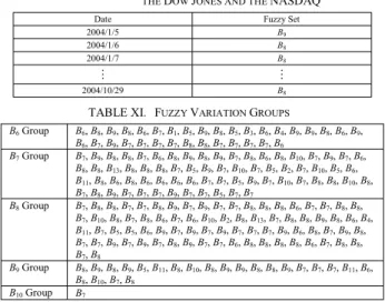
Step 6.3: Based on the linguistic terms of the fuzzified variations, group the fuzzy variation of the main factor on trading day t having the same linguistic term of the fuzzy variation of the secondary factor on trading t − 1. For example, let us consider the following fuzzy variation between the

secondary factor on trading day t − 1 and the main factor on trading day t: the fuzzy variation of the main factor on trading day t is “B _b1 ” and the fuzzy variation of the secondary factor on trading day t − 1 is B z ; the fuzzy variation of the main factor on trading day t + m is “B _b2 ” and the fuzzy variation of the secondary factor on trading day t + m − 1 is B ^z ; …; the fuzzy variation of the main factor on trading day t + n is “B _bk ” and the fuzzy variation of the secondary factor on trading day t + n − 1 is B z . Then, these fuzzy variations of the main factor can be grouped into the same fuzzy variation group of the secondary factor in which each fuzzy variation of the secondary factor in this group is B z , shown as follows:

B b1 , B b2 , …, B bk .

For example, from Table X and Table VII, we can see that the fuzzy variation of the secondary factor on 2004/1/5 is B 9 and the fuzzy variation of the main factor on 2004/1/6 is B 8 . We can then group the fuzzy variation of the main factor “B 8 ” into the fuzzified variation of the secondary factor B 9 group. Table XI shows the fuzzy variation groups with respect to different fuzzified variations of the secondary factor.

TABLE X. F UZZIFIED V ARIATIONS OF THE S ECONDARY F ACTOR

“ THE D OW J ONES AND THE NASDAQ”

Date Fuzzy Set

2004/1/5 B

9

2004/1/6 B

8

2004/1/7 B

8

# #

2004/10/29 B

8

TABLE XI. F UZZY V ARIATION G ROUPS

B

6

Group B

6

, B

8

, B

9

, B

8

, B

6

, B

7

, B

1

, B

5

, B

9

, B

8

, B

5

, B

3

, B

6

, B

4

, B

9

, B

9

, B

8

, B

6

, B

9

, B

6

, B

7

, B

9

, B

7

, B

7

, B

7

, B

7

, B

8

, B

8

, B

7

, B

7

, B

7

, B

7

, B

6

B

7

Group B

7

, B

9

, B

8

, B

8

, B

7

, B

6

, B

8

, B

9

, B

8

, B

9

, B

7

, B

8

, B

6

, B

8

, B

10

, B

7

, B

9

, B

7

, B

6

, B

8

, B

8

, B

13

, B

8

, B

8

, B

8

, B

7

, B

5

, B

9

, B

7

, B

10

, B

7

, B

5

, B

2

, B

7

, B

10

, B

5

, B

6

, B

11

, B

8

, B

6

, B

8

, B

6

, B

6

, B

6

, B

6

, B

7

, B

7

, B

5

, B

9

, B

7

, B

10

, B

7

, B

8

, B

8

, B

10

, B

8

, B

7

, B

8

, B

9

, B

7

, B

7

, B

7

, B

9

, B

7

, B

7

, B

5

, B

7

, B

7

B

8

Group B

7

, B

8

, B

8

, B

7

, B

7

, B

8

, B

9

, B

7

, B

9

, B

7

, B

7

, B

8

, B

8

, B

8

, B

6

, B

7

, B

7

, B

8

, B

8

, B

7

, B

10

, B

8

, B

7

, B

8

, B

6

, B

7

, B

6

, B

10

, B

2

, B

8

, B

13

, B

7

, B

8

, B

8

, B

9

, B

8

, B

6

, B

4

, B

11

, B

7

, B

5

, B

5

, B

6

, B

9

, B

7

, B

9

, B

7

, B

9

, B

7

, B

7

, B

7

, B

9

, B

6

, B

8

, B

7

, B

9

, B

8

, B

7

, B

7

, B

9

, B

7

, B

9

, B

7

, B

8

, B

9

, B

7

, B

7

, B

6

, B

8

, B

8

, B

8

, B

8

, B

6

, B

7

, B

8

, B

8

, B

7

, B

8

B

9

Group B

8

, B

9

, B

8

, B

9

, B

5

, B

11

, B

8

, B

10

, B

8

, B

9

, B

9

, B

8

, B

8

, B

9

, B

7

, B

7

, B

7

, B

11

, B

6

, B

8

, B

10

, B

7

, B

8

B

10

Group B

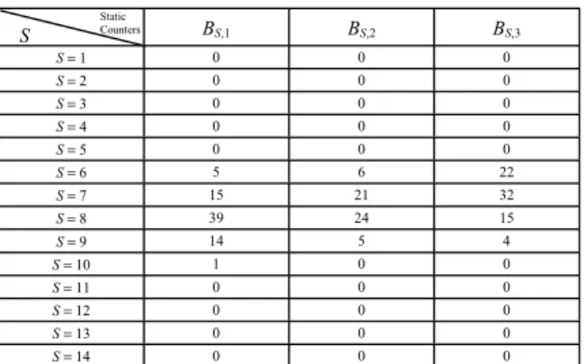
7

Step 6.4: Evaluate the linguistic terms of the fuzzy variation groups between the secondary factor and the main factor. Let the fuzzy variations of the main factor and the secondary factor be B M and B S , respectively, where M and S are positive numbers, 1 ≤ M ≤ 14 and 1 ≤ S ≤ 14. Let B S,1 be the static counter denoting the number of fuzzy variations in the B S

Group and M < S; let B S,2 be the static counter denoting the number of fuzzy variations in the B S Group and M = S; let B S,3

be the static counter denoting the number of fuzzy variations in the B S Group and M > S, where B S,1 , B S,2 and B S,3 are integers whose initial values are 0. Evaluate the fuzzy variation B S

groups in which the effect between the secondary factor and the main factor appear, described as follows:

Situation 1: In the B S Group, if M < S, then we can see that when the secondary factor is B S , the index M of the fuzzy variation of the main factor is less than S. We add one to the B _S,1 when the secondary factor is B _S and M < S.

Situation 2: In the B S Group, if M = S, then we can see that

when the secondary factor is B _S , the index M of the fuzzy

variation of the main factor M is equal to S. We add one to the B _S,2 when the secondary factor is B _S and M = S.

Situation 3: In the B S Group, if M > S, then we can see that when the secondary factor is B _S , the index M of the fuzzy variation of the main factor is bigger than S. We add one to the B _S,3 when the secondary factor is B _S and M > S.

For example, we let the TAIEX be the main factor and let “the Dow Jones and the NASDAQ” be the secondary factor. From the B ₆ Group shown in Table XI, we can see that the fuzzy variations of the main factor are B ₆ , B ₈ , B ₉ , B ₈ , B ₆ , B ₇ , B ₁ , B ₅ , B ₉ , B ₈ , B ₅ , B ₃ , B ₆ , B ₄ , B ₉ , B ₉ , B ₈ , B ₆ , B ₉ , B ₆ , B ₇ , B ₉ , B ₇ , B ₇ , B ₇ , B ₇ , B ₈ , B ₈ , B ₇ , B ₇ , B ₇ , B ₇ and B ₆ . Because S is 6 and the situation when M < S are B ₁ , B ₅ , B ₅ , B ₃ and B ₄ , the total number of fuzzy variations is 5, i.e., B 6,1 = 5. In the same way, the situation when M = S are B 6 , B 6 , B 6 , B 6 , B 6 and B 6 , the total number of fuzzy variations number is 6, i.e., B 6,2 = 6. In the same way, the situation when M > S are B 8 , B 9 , B 8 , B 7 , B 9 , B 8 , B 9 , B 9 , B 8 , B 9 , B 7 , B 9 , B 7 , B 7 , B 7 , B 7 , B 8 , B 8 , B 7 , B 7 , B 7 and B 7 , the total number of fuzzy variations is 22, i.e., B 6,3 = 22.

Table XII shows the statistics of the fuzzy variations of the secondary factor “the Dow Jones and the NASDAQ”, where the main factor is the TAIEX.

TABLE XII. T HE S TATISTICS OF THE F UZZY V ARIATIONS OF THE

S ECONDARY F ACTOR “ THE D OW J ONES AND THE NASDAQ”,

WHERE THE M AIN F ACTOR IS THE TAIEX

B

S,1

B

S,2

B

S,3

S = 1 0 0 0

S = 2 0 0 0

S = 3 0 0 0

S = 4 0 0 0

S = 5 0 0 0

S = 6 5 6 22

S = 7 15 21 32

S = 8 39 24 15

S = 9 14 5 4

S = 10 1 0 0

S = 11 0 0 0

S = 12 0 0 0

S = 13 0 0 0

S = 14 0 0 0

Step 7: Define the weights of the fuzzy variation B s of the secondary factor when S > M, S = M, and S < M. According to Step 6.4 , we let B S,1 be the total number of times when the secondary factor is B _S and S > M; let B _S,2 be the total number of times when the secondary factor is B _S and S = M; let B S,3 be the total number of times when the secondary factor is B _S and S <

M. Let W _Bs,1 , W _Bs,2 and W _Bs,3 be the weights of the fuzzy set B _S at different situations, where W _Bs,1 denotes the weight of B _S when S > M; W Bs,2 denotes the weight of B S when S = M; W ^Bs,3 denotes the weight of B _S when S < M. The weight of the fuzzy variation B _S,k is calculated as follows:

,3 s ,2 s ,1 s

k , s k ,

Bs

B B B

W B

+

= + , (3)

where k is a positive integer and k = 1, 2, 3. For example, from Table XII, we can see that the number of times is 5 when the fuzzy variation is B 6 and S > M; the number of times is 6 when the fuzzy variation is B 6 and S = M; the number of times is 22 when the fuzzy variation is B 6 and S < M. Therefore, the weight W B6,1 is equal to

22 6 5

5 +

+ = 0.151515, the weight W B6,2 is equal to

22 6 5

6 +

+ = 0.181818, and the weight W B6,3 is equal to

22 6 5

22 +

+ =

0.666667. In summary, the weights of the fuzzy variation B _j of the secondary factor are shown in Table XIII, where 1 ≤ j ≤ 14.

Step 8: Assume that the main factor F(t −1) = A i and assume that we want to predict the main factor F(t), where A _i is a fuzzy set. Based on the fuzzy variation of the secondary factor F(t −1)

= B j , we choose the corresponding fuzzy variation B j of the weight of the secondary factor of the fuzzy logical relationship groups for prediction. Assume that the fuzzy variation of the secondary factor of the trading day t −1 is B j . We then choose the fuzzy logical relationship: “A i → A i1 , A i2 , …, A iz ” in the Group B j . Let u i1 L

, u i2 L

, …, and u iz L

be the minimum value of the intervals u i1 , u i2 , …, and u iz , respectively; let u i1 M

, u i2 M

, …, and u iz M

be the midpoints of the intervals u i1 , u i2 , …, and u iz , respectively; let u i1 R

, u i2 R

, …, and u iz R

be the maximum value of the intervals u i1 , u i2 , …, and u iz , respectively. The new value u a * of u a is calculated as follows:

u a * = W Bj,1 × u a L

+ W Bj,2 × u a M

+ W Bj,3 × u a R

, (4) where a = i1, i2, …, iz, and the forecasted value FV of day t is calculated as follows:

z

* u FV

iz i a ¦ a

= ^{= 1} . (5)

TABLE XIII. T HE W EIGHTS OF THE F UZZY V ARIATION B

S,K

OF THE

S ECONDARY F ACTOR

k = 1 k = 2 k = 3

W

B1,k

0 0 0

W

B2,k

0 0 0

W

B3,k

0 0 0

W

B4,k

0 0 0

W

B5,k

0 0 0

W

B6,k

0.151515 ʳ 0.181818 0.666667

W

B7,k

0.220588 0.308824 0.470588

W

B8,k

0.5 0.307692 0.192308

W

B9,k

0.608696 0.217391 0.173913

W

B10,k

1 0 0

W

B11,k

0 0 0

W

B12,k

0 0 0

W

B13,k

0 0 0

W

B14,k

0 0 0

For example, assume that we want to forecast the TAIEX of 2004/11/2 by the first order fuzzy logical relationships. From Table I and Table XIII we can see that because the TAIEX on 2004/11/1 is 5656.17 (Note: Its fuzzified TAIEX is A 4 ) and because from Table V, we can see that the variation of the Dow Jones and the NASDAQ on 2004/11/1 are 0.268463 % and 0.247090 %, respectively, based on Step 6.1, the variation of the secondary factor is

2

% 247090 0

% 268463

0 . + . = ^{0 . 515553} ₂ ^% = 0.257777

% and based on Table VI, we can see that the fuzzy variation of the secondary factor is B 8 . We choose the B 8 group shown in Table VIII, where the left-hand side of the fuzzy logical relationship “A ₄ → ^A 5 , A ₄ , A ₄ , A ₄ , A ₅ ” is A ₄ . The given weights u ₅ and u ₄ become u ₅ * and u ₄ *, respectively, for forecasting. The minimum value of the interval u ₅ is 5700, the midpoint of the interval u ₅ is 5750 and the maximum value of the interval u ₅ is 5800. Based on Eq. (3), we can get the weight of B _8,1 = 0.5, the weight of B _8,2 = 0.307692 and the weight of B _8,3 = 0.192308.

Based on Eq. (4), the new value u ₅ * of u ₅ for prediction is calculated as follows: 5700 × 0.5 + 5750 × 0.307692 + 5800 × S

Static Counters

Weight of Fuzzy Set

k

0.192308 = 5734.62. In the same way, we can get u 4 * = 5634.62. Finally, based on Eq. (5), the forecasted TAIEX of 2004/11/2 is calculated as follows:

. 62 5674 5

62 5734 62 5634 62 5634 62 5634 62

5734 . + . + . + . + . = .

IV. E XPERIMENTAL R ESULTS

In this section, we apply the proposed method to forecast the TAIEX from 2000 to 2004. We evaluate the performance of the proposed method using the root mean square error (RMSE), which is defined as follows:

n

value actual value forecasted RMSE

n

i ¦ i − i

= ⁼¹

) 2 (

, (6) where n denotes the number of dates needed to be forecasted.

In Table XIV, we make a comparison of the RMSE and the average RMSE of the proposed method with Chen’s method [1] and Huarng et al.’s method [9]. From Table XIV, we can see that the proposed method with “the Dow Jones and the NASDAQ” gets the smallest average RMSE compared to Chen’s method [1] and Huarng et al.’s method [9]. It means that the proposed method with the Dow Jones and the NASDAQ gets a higher average forecasting accuracy rate than Chen’s method [1] and Huarng et al.’s method [9].

TABLE XIV. A C OMPARISON OF THE RMSE S AND THE A VERAGE RMSE

FOR D IFFERENT M ETHODS

2000 2001 2002 2003 2004 Average RMSE Chen's Method [1] 176.32 147.84 101.18 74.46 84.28 116.82 Huarng et al.’s Method (use

NASDAQ) [9] 158.7 136.49 95.15 65.51 73.57 105.88 Huarng et al.’s Method (use Dow

Jones) [9] 165.8 138.25 93.73 72.95 73.49 108.84 Huarng et al.’s Method (use M

_1b

)

[9] 169.19 133.26 97.1 75.23 82.01 111.36 Huarng et al.’s Method ( use

NASDAQ & Dow Jones) [9] 157.64 131.98 93.48 65.51 73.49 104.42 Huarng et al.’s Method (use

NASDAQ & M

1b

) [9] 155.51 128.44 97.15 70.76 73.48 105.07 Huarng et al.’s Method (use

NASDAQ & Dow Jones & M

1b

) [9]

154.42 124.02 95.73 70.76 72.35 103.46 The Propose Method (use Dow

Jones) 127.51 121.98 74.65 66.02 58.89 89.81 The Propose Method (use

NASDAQ) 129.87 123.12 71.01 65.14 61.94 90.22 The Propose Method (use M

1b

) 129.87 117.61 85.85 63.1 67.29 92.74 The Propose Method (use Dow

Jones & NASDAQ) 124.06 125.12 72.25 57.14 56.95 87.10 The Propose Method (use Dow

Jones and M

1b

) 127.75 115.64 79.45 60.41 65.86 89.82 The Propose Method (use

NASDAQ and M

_1b

) 128.45 126.14 76.03 66.96 65.5 92.62 The Propose Method (use Dow

Jones, NASDAQ and M

1b

) 129.57 119.66 73.25 66.8 65.41 90.94

V. C ONCLUSIONS

In this paper, we have presented a new method to forecast the Taiwan Stock Exchange Capitalization Weighted Stock Index (TAIEX) based on fuzzy time series. From Table XIV, we can see that the proposed method with the Dow Jones and the NASDAQ gets a higher average forecasting accuracy rate than Chen’s method [1] and Huarng et al.’s method [9] for forecasting the TAIEX. The experimental results show that the proposed method gets a higher average forecasting accuracy rate than the methods, presented in [1] and [9].

A CKNOWLEDGMENT

This work is supported in part by the National Science Council, Republic of China, under Grant NSC 97-2221-E-011- 107-MY3.

R EFERENCES

[1] S. M. Chen, “Forecasting enrollments based on fuzzy time series,”

Fuzzy Sets and Systems, vol. 81, no. 3, pp. 311-319, 1996.

[2] S. M. Chen, “Forecasting enrollments based on high-order fuzzy time series,” Cybernetics and Systems, vol. 33, no. 1, pp. 1-16, 2002.

[3] S. M. Chen and N. Y. Chung, “Forecasting enrollments using high- order fuzzy time series and genetic algorithm,” International Journal of Intelligent Systems, vol. 21, no. 5, pp. 485-501, 2006.

[4] S. M. Chen and C. C. Hsu, “A new method to forecast enrollments using fuzzy time series,” International Journal of Applied Science and Engineering, vol. 2, no. 3, pp. 234-244, 2004.

[5] S. M. Chen and J. R. Hwang, “Temperature prediction using fuzzy time series,” IEEE Transactions on Systems, Man, and Cybernetics-Part B:

Cybernetics, vol. 30, no. 2, pp. 263-275, 2000.

[6] S. M. Chen and N. Y. Wang, “Handling forecasting problems based on high-order fuzzy time series and fuzzy-trend logical relationships,”

Proceedings of the 2008 Workshop on Consumer Electronics, Taipei County, Taiwan, Republic of China, pp. 759-764, 2008.

[7] K. Huarng, “Effective lengths of intervals to improve forecasting in fuzzy time series,” Fuzzy Sets and Systems, vol. 123, no. 3, pp. 387- 394, 2001.

[8] K. Huarng and H. K. Yu, “Ratio-based lengths of intervals to improve fuzzy time series forecasting,” IEEE Transactions on Systems, Man, and, Cybernetics-Part B: Cybernetics, vol. 36, no. 2, pp. 328-340, 2006.

[9] K. Huarng, H. K. Yu, and Y. W. Hsu “A multivariate heuristic model for fuzzy time-series forecasting,” IEEE Transactions on Systems, Man, and, Cybernetics Part-B: Cybernetics, vol. 37, no. 4, pp. 836-846, 2007.

[10] L. W. Lee, L. H. Wang, S. M. Chen, and Y. H. Leu, “Handling forecasting problems based on two-factors high-order fuzzy time series,” IEEE Transactions on Fuzzy Systems, vol. 14 , no. 3, pp. 468- 477, 2006.

[11] Q. Song and B. S. Chissom, “Fuzzy time series and its model,” Fuzzy Sets and Systems, vol. 54, no. 3, pp. 269-277, 1993.

[12] Q. Song and B. S. Chissom, “Forecasting enrollments with fuzzy time series - Part I,” Fuzzy Sets and Systems, vol. 54, no. 1, pp. 1-9, 1993.

[13] Q. Song and B. S. Chissom, “Forecasting enrollments with fuzzy time series - Part II,” Fuzzy Sets and Systems, vol. 62, no. 1, pp. 1-8, 1994.

[14] N. Y. Wang and S. M. Chen, “Temperature prediction and TAIFEX forecasting based on automatic clustering techniques and two-factors high-order fuzzy time series,” Expert Systems with Applications, vol.

36, no. 2, pp. 2143-2154, March 2009.

[15] N. Y. Wang, S. M. Chen, and J. S. Pan, “Forecasting enrollments based on automatic clustering techniques and fuzzy time series,” Proceedings of the 12th Conference on Artificial Intelligence and Applications, Yunlin, Taiwan, Republic of China.

[16] H. K. Yu, “A refined fuzzy time-series model for forecasting,” Physica A, vol. 346, no. 3-4, pp. 657–681, 2004.

[17] H. K. Yu, “Weighted fuzzy time-series models for TAIEX forecasting,” Physica A, vol. 349, no. 3-4, pp. 609–624, 2004.

[18] H. K. Yu and K. H. Huarng, “A bivariate fuzzy time series model to forecast the TAIEX,” Expert Systems with Applications, vo1. 34, no. 4, pp. 2945-2952, 2008.

[19] I. H. Kuo, S. J. Horng, T. W. Kao, T. L. Lin, C. L. Lee, and Y. Pan,

“An improved method for forecasting enrollments based on fuzzy time series and particle swarm optimization,” Expert Systems with Applications, vo1. 36, no. 3, pp. 6108-6117, 2009.

[20] H. J. Teoh, T. L. Chen, C. H. Cheng, and H. H. Chu, “A hybrid multi- order fuzzy time series for forecasting stock markets,” Expert Systems with Applications, vo1. 36, no. 4, pp. 7888-7897, 2009.

[21] L. A. Zadeh, “Fuzzy sets,” Information and Control, vol. 8, pp. 338- 353, 1965.

Year RMSE

Methods