Reversible data hiding for high quality images exploiting interpolation and direction order mechanism

Reversible Data Hiding For High Quality Images Exploiting Interpolation and Direction Order Mechanism

Xing-Tian Wang ^a , Chin-Chen Chang ^b,c,* , Thai-Son Nguyen ^d and Ming-Chu Li ^e

a Department of Software Dalian University of Technology

DaLian, China

E-Mail: wxt6582295@gmail.com

b Department of Information Engineering and Computer Science Feng Chia University

Taichung City 407, Taiwan

c Department of Biomedical Imaging and Radiological Science Chinese Medical University

Taichung City 404, Taiwan

* Corresponding author: alan3c@gmail.com

d Department of Information Engineering and Computer Science Feng Chia University

Taichung City 407, Taiwan E-Mail: thaison@tvu.edu.vn

e Department of Software Dalian University of Technology

DaLian, China

E-Mail: li_mingchu@yahoo.com

Abstract

Reversible data hiding can restore the original image from the stego image without any distortion after the embedded secret message is exactly extracted. In this paper, a novel, reversible, data hiding scheme for high quality images is proposed in spatial domain. To increase embedding capacity and enhance image quality, the proposed scheme classifies all pixels as wall pixels and non-wall pixels. For wall pixel, the interpolation error is used to embed secret data over the interpolation prediction method. In contrast, the difference value between the non-wall pixel and its parent pixel, which is defined by the direction order, is computed to hide secret data based on the histogram shifting. The experimental results demonstrate that our scheme provides the larger payload and the better image quality than some existing schemes. Moreover, the performance of the proposed scheme is more stable for the different images.

Keywords: reversible data hiding, histogram modification, interpolation error, direction order,

steganography

1. Introduction

Digitization and networking have become more and more evident characteristics in the rapid development of the economic society. The convenient and timely acquisition of on-line services through accessing the Internet is a tidal current for individuals and organizations. However, the transmission of sensitive information via an open Internet channel increases the risk of interception. Thus many techniques have been proposed to deal with this issue. Data hiding, known as information hiding, plays an important role in information security. The main idea of data hiding is that the secret data is concealed into the cover medium, such as an image, audio, video or text, to avoid attracting the attention of attackers in the Internet channel, who may capture the secret data for malicious purposes.

Some literatures proposed varieties of data hiding techniques. Most of them are irreversible [1-3]. It means that, after the secret data are extracted from the stego image, the original image is injured with some distortion and cannot be completely reconstructed. Nevertheless, in some fields (i.e., medical, military applications), the restoration of original image is essential after extracting the embedded secret data. Therefore, reversible data hiding schemes [4-19], also called as distortion-free data hiding or lossless data hiding, have drawn much attention of researchers. In principle, reversible data hiding schemes can be classified into three types, i.e., spatial domain, frequency domain, and compressed domain. In the spatial domain schemes [4, 9, 10, 12-19], all pixel values are modified directly to embed secret data. In the frequency domain schemes, the coefficient values of image are computed by using some transformation methods (i.e., integer discrete cosine transform [6], integer wavelet transform [7]). These coefficient values are modified in order to embed secret data into the cover image. In the compressed domain schemes, the original image is first compressed based on some popular compression algorithms, such as vector quantization [5, 11], block truncation coding [8]. Then, according to the peculiarity of compressed codes, the compressed image is encoded to conceal secret data.

Most reversible data hiding, in the spatial domain, based on difference expansion (DE) [9, 10, 12, 13] and histogram shifting [4, 14-19]. Basically, the schemes belonged to DE give the larger embedding capacity. In contrast, the schemes belonged to histogram shifting provide the better visual quality of stego image. Over last five years, some reversible data hiding schemes [4, 14-19]

based on the histogram shifting, which was first proposed by Ni et al. [16] in 2006, have been

presented. Since most of the pixels, in Ni et al.’s scheme, are modified by one grayscale value, the scheme achieves high visual quality of stego image. However, Ni et al.’s scheme provides limited embedding capacity. To obtain better embedding performance, in 2009, Tsai et al. [15] divided the cover image into some blocks and shifted the differences between the reference pixel and other pixels in each block for concealing secret data. In the same year, Kim et al. [4] proposed the reversible data hiding scheme based on the difference histogram shifting. In Kim et al.’s scheme, the original image is divided into several sub-images. Then the difference values between the sub- sampled images are modified to embed more secret message. To improve Kim et al.’s scheme, Luo et al. [4] selected the median pixel of each block to structure the reference sub-image.

However, since the reference sub-image or reference pixels are not used to carry secret data, the embedding capacity of these schemes is limited. In 2010, Li et al. [14] introduced a new reversible data hiding scheme by depending on the differences of adjacent pixels. In this scheme, the histogram of the difference sequence of pixels is explored to embed secret data. A reversible data hiding scheme, presented by Zhao et al. [17] in 2011, employed the multilevel histogram modification mechanism to embed secret data into more bins.

In this paper, a novel, reversible, data hiding scheme based on histogram shifting is presented to further improve embedding capacity and image quality. In our scheme, All pixels are classified into two types, i.e., wall pixels and non-wall pixels. To conceal secret data, the interpolation errors [19] are performed for the wall pixels. Also, calculate the difference values between the non-wall pixels and their corresponding parent pixels, which are defined according to the direction order, based on the histogram shifting. Experimental results confirm that our scheme can provide larger embedding payload while maintaining better visual quality of the stego image.

The remainder of this paper is organized as follows. Section 2 will review the reversible data hiding scheme of Luo et al. [18]. Then, the proposed scheme is depicted at length in Section 3.

Section 4 shows the experimental results and relevant discussions. Finally, the conclusions are given in Section 5.

2. Related Work

In this section, Luo et al.’s scheme [18] is briefly reviewed. Suppose that the host image I is

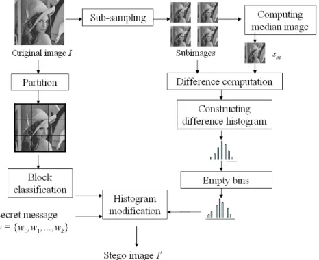
an 8-bit gray level image in the size of N´M. The flowchart of data embedding algorithm of Luo et

al.’s scheme is shown in Figure 1.

=============================Figure 1===================================

Figure 1. Flowchart of data embedding algorithm Data embedding algorithm

Input: Original image I.

Output: Stego image I.

Step 1: Partition and sub-sample image I. It means that, in this step, image I will be partitioned into a set of u´v blocks. Besides, sub-sample image I into sub-images s 1 , s 2 , …, s u´v

with each sized ⌊ ^{N u} ⌋ ^× ⌊ ^{M v} ⌋ _.

Step 2: Compute median image s m . First, retrieve s 1 (i, j), s 2 (i, j), …, s u´v (i, j) to create pixel array. Then, this pixel array is sorted in ascending order (i.e., p 1 (i, j)  p 2 (i, j)  …  p u´v (i, j)).

Media image s m is calculated by using Equation (1).

s _m (i, j)= p

⌊ ^{u×v+1 2} ⌋ ^{(i , j)} . (1) Step 3: Block classification. All blocks (i.e., s 1 (i, j), s 2 (i, j), …, s u´v (i, j)) can be classified into two types, Type I and Type II. Assume that n l , n 0 , n r denote the numbers of pixel values smaller, equal and larger than s m (i, j) in a block, respectively. Table 1 presents the block classification based on median.

Table 1. Block classification based on median

=================================Table 1==============================

Step 4: Calculate the difference between s m (i, j) and other (u´v) - 1 pixels by Equation (2).

d _k ( i, j )=s _k (i, j )−s _m (i , j) , (2) where 1  k  u´v, k  m.

Step 5: According to all calculated differences, construct the difference histogram.

Step 6: Fix on the embedding level (EL). Then, the bins in the range of [b -2EL-1 , b -EL-1 ] and [b EL+1 , b 2EL+1 ] are emptied by Equation (3).

d _k ( i , j )+ EL if d _k ( i , j )> EL , d _k ( i , j )− EL if d _k ( i , j )<− EL ,

d _k (i , j ) otherwise,

¿

d _k

(i , j )=¿ ^{ ¿ ^{ ¿ ¿ ¿

¿ (3)

where 1  k  u´v, k  m. By using Equation (3), the block composed by s 1 (i, j), s 2 (i, j),…, s u´v (i, j)

can be modified as Equation (4).

s _k ( i , j )+ EL if s _k ( i , j )> s _m ( i , j )+ EL , s _k ( i , j )− EL if s _k ( i , j )< s _m ( i , j )− EL ,

s _k ( i , j ) otherwise,

¿ s _k

=¿ ^{ ¿ ^{ ¿ ¿ ¿

¿ (4)

where 1  k  u´v, k  m, and s ^{k '} ( i, j ) indicates the modified pixel value after empting bins.

Step 7: Histogram shifting is the main operation of data embedding. The strategies of embedding data are described according to block type as follows. We take the example of EL = 2.

(1) Type I.

Secret bit w can be embedded by repeating Equation (5) for EL = 2 first and EL = 1 second, respectively.

s

( i , j ) + EL+ w if { s s

( i , j )− EL−w if { s ¿

¿

¿

s

( i , j )= ¿ { ^{¿ '}

( i , j )− s

( i , j ) = EL , ¿ ¿ ¿

¿ (5)

where 1  k  u´v, k  m.

(2) Type II-1.

For EL = 2 first and then EL = 1, secret bit w can be embedded by repeating Equation (5).

When EL = 0, calculate

s

( i , j )+ ( −1 )

if { s s

( i , j ) if { s ¿

¿

¿

s

( i , j )= ¿ { ^{¿ '}

( i , j )= s

( i , j ) , w =1, ¿ ¿ ¿

¿ (6)

where 1  k  u´v, k  m, and q describes the qth encountered s k (i, j) equaling s m (i, j) (k  m).

(3) Type II-2.

When EL > 0, secret bit w can be embedded by repeating Equation (5) for EL = 2 and EL = 1, respectively. When EL = 0, Equation (7) is used to embed secret bit w.

s

(i , j )−1 if { s

¿

s

(i , j )+(−1 )

if { s

¿

s

(i , j ) if { s

¿

¿

s

(i , j )=¿ { ^¿'

(i , j )= s

(i , j ) , w =1, q<n

−n

, ¿ { ^{¿ '}

(i , j )= s

(i , j ) , w= 1,q ≥n

−n

, ¿ ¿ ¿

¿ (7)

where 1  k  u´v, k  m, and q has the same meaning as that in Type II-1.

(4) Type II-3.

When EL > 0, repeat Equation (5) for EL = 2 and EL = 1, respectively. When EL = 0, use

Equation (8) to embed secret bit w.

s

(i , j )+1 if { s

¿

s

(i , j )−(−1)

if { s

¿

s

(i , j ) if { s

¿

¿

s

(i , j )=¿ { ^¿'

(i , j )= s

(i , j ) , w =1, q≤ n

−n

, ¿ { ^{¿ '}

(i , j )= s

(i , j ) , w =1, q>n

−n

, ¿ ¿ ¿

¿ (8)

where 1  k  u´v, k  m, and q has the same meaning as that in Type II-1.

Step 8: Recompose the sub-images s ^{1 ' '} ,s ₂ ^'' ,...,s _u×v ^{' '} to generate the stego image I.

After the above mentioned 8 steps are processed completely, the stego image I can be obtained. Then, this image is sent to the receiver without any extra information. The reverse steps will be implemented to extract the secret message and recover the original image.

3. Proposed scheme

In this section, a histogram-based reversible data hiding scheme is proposed in spatial domain.

To achieve better embedding efficiency, in our scheme, the pixels of cover image are first classified into two types, i.e., wall pixels and non-wall pixels as shown in Figure 2. The distance of two neighboring wall pixels is denoted as . For example,  is 1 in Figure 2. Denote pixel at coordinate (i, j) as P(i, j), so P(i, j) is a wall pixel when mod(i,  + 1) = 0 and mod(j,  + 1) = 0, where mod(x, y) represents x modulo y. Otherwise, P(i, j) is a non-wall pixel.

==============================Figure 2==================================

Figure 2. Pixel classification

3.1. Data embedding procedure

After pixel classification, wall pixels are first embedded secret message B 1 implementing interpolation errors [19]. Then, non-wall pixels are embedded extra information E, and secret message B 2 based on the difference of adjacent pixels. During embedding, pixels 0 and 255 may be changed to -1 and 256, respectively. Hence, the overflow and underflow problems may occur.

To deal with the saturated problem, first scan the cover image by successive lines before

embedding. If the value of encountered pixel is 0 or 255, it is shifted to 1 or 254, and one indicator

bit 1, denoted as Ib = 1, is output to extra information E. If the value of encountered pixels is 1 or

254, one indicator bit 0, i.e., Ib = 0, is sent to extra information E. After scan, we can obtain a

complete extra information E = (Ib 1 , Ib 2 , …, Ib x ). In the recovery, we can restore these shifted

pixels according to the extra information. If Ib i = 1, the i-th encountered pixel through scanning the stego image by successive lines, the value of which is 1 or 254, is restored to 0 or 255. If Ib i = 0, it means that the i-th encountered pixel, whose value is 1 or 254, does not be shifted in the pre- processing, so its value is reserved. In the pre-processing, if a cover image does not contain any boundary pixel 0 and 255, the size of extra information is 0. Hence, we use one bit to record whether the extra information exists. We will discuss it later. After pre-processing, the processed image will be embedded secret data without overflow or underflow. Figure 3 shows the overall flowchart of data embedding algorithm.

=================================Figure 3===============================

Figure 3. Flowchart of data embedding algorithm

The data embedding algorithm is divided into nine steps as follows:

Data embedding algorithm

Input: Original image I, secret message B.

Output: Stego image I, side information.

Step 1: Pre-process the cover image through scanning it by successive lines to obtain the extra information E. Classify all pixels of the pre-processed image as wall pixels and non-wall pixels. For convenient explanation, we denote the section of secret message embedded into wall pixels as B 1 , and the remainder of B as B 2 . Therefore, the secret message B 1 will be embedded into wall pixels, while the new secret message M, including E and B 2 , is embedded into non-wall pixels.

Step 2: For wall pixel P, the interpolation prediction method is used to generate its interpolation value P pre by two pairs of neighboring non-wall pixels along orthogonal direction of 0 ^ and ^{90 } . Then, subtract the corresponding interpolation value P pre from the wall pixel P at coordinate (i, j) to obtain interpolation error e, i.e., e(i, j) = P(i, j) – P pre (i, j).

Step 3: The histogram of interpolation errors of all wall-pixels is constructed, resembling the

show in Figure 4. In the histogram, the range of error value is from -255 to +255. Then, two pairs

of peak and zero points are selected as follows. The two most frequent error values, known as two

peak points, are selected and denoted as He 1 and He 2 , where He 2 < He 1 . Denote the smallest error

value, whose frequency is 0, in range of [He 1 , 255] as zero point Ze 1 , and denote the largest error

value, whose frequency is 0, in range of [-255, He 2 ] as zero point Ze 2 .

================================Figure 4================================

Figure 4. Histogram of interpolation errors of wall-pixels

Step 4: To embed secret message, the histogram will be shifted as follows. First empty the bins of (He 1 + 1) and (He 2 – 1). All error values in range of [He 1 + 1, Ze 1 – 1] of histogram is shifted to right by 1 unit, and all error values in range of [Ze 2 + 1, He 2 – 1] of histogram is shifted to left by 1 unit, resembling the show in Figure 5. Then, the secret message B 1 will be embedded into the bins of He 1 and He 2 . The modified error e at coordinate (i, j) can be calculated using Equation (9) to embed each secret bit b of B 1 .

e( i , j )+1 if He ₁ +1≤e (i , j )≤Ze ₁ −1;

e( i , j )− 1 if Ze ₂ +1≤e ( i , j )≤He ₂ − 1;

e ( i , j ) if e( i , j )= He ₁ or e( i , j )= He ₂ , and b=0 ; e( i , j )+1 if e ( i , j )= He ₁ and b=1;

e ( i , j )−1 if e (i , j )= He ₂ and b=1 ; e( i , j ) otherwise .

¿

e ^' (i , j )=¿ ^{ ¿ ^{ ¿ ^{ ¿ ^{ ¿ ^{ ¿ ¿ ¿

¿ (9)

=================================Figure 5===============================

Figure 5. Shifted histogram of interpolation errors of wall-pixels

Step 5: For non-wall pixels, the processed order of pixels is arranged according to the direction order as shown in Figure 6. For better explanation, an example is taken as shown in Figure 7. First, we will begin from the start pixel, and we denote it as P 1 . According to direction order, since the pixels derived from the first and second directions of P 1 are wall pixels, the pixel having index 2, denoted as P 2 , will come from the third direction of P 1 . Then, we can consider P 2

as the child pixel of P 1 . In other words, P 1 is the parent pixel of P 2 . For P 2 , the subsequence of it

from the first direction is non-wall pixel and never has been used before. Therefore, P 3 originated

from the first direction of P 2 is set up. It means that P 2 is the parent pixel of P 3 . In the same way,

P 3 and P 4 are the parent pixels of P 4 and P 5 , respectively. For P 5 in Figure 7, it does not have the

first direction, and the pixel from the second direction of P 5 is already processed. Besides, the

third and fourth directions of P 5 are wall pixels. Therefore, we turn back from P 5 to its parent pixel

P 4 . Then, since the third direction of P 4 is available, we can set the subsequence of P 4 from its third

direction as P 6 . Hence, P 5 and P 6 are both the child pixels of P 4 . Certainly, P 14 is also the child pixel of P 4 . Similarly, P 10 has three child pixels, such as P 11 , P 12 and P 13 . According to the regulation of direction order, it is found that a pixel at most has three child pixels, and has exactly only one parent pixel excluding the start pixel.

=================================Figure 6===============================

Figure 6. Direction order

================================Figure 7================================

Figure 7. Processed order of pixels based on direction order

Step 6: Compute the non-wall difference values as follows. In Equation (10), for the current pixel P k at coordinate (i, j), its difference value d k is calculated by subtracting the value of its parent pixel from that of it, where k≠1 , it means that the start pixel has no difference value and it is reserved for the initial condition of extraction. Since each pixel has only one parent pixel, the difference value of P k is unique.

d _k (i, j )=P _k (i, j )−( P _k (i , j)) ^o _pare , (10) where ( P _k ( i , j)) ^o _pare represents, for the current being processed pixel P k at coordinate (i, j), the value of P k ’s parent pixel of original image.

Step 7: Construct the histogram of difference values of non-wall pixels. In this histogram, the range of difference value is from -255 to +255. Similar to Step 3, two pairs of peak and zero points are selected as follows. The two most frequent difference values, known as two peak points, are selected and denoted as Hd 1 and Hd 2 , where Hd 2 < Hd 1 . Denote the smallest difference value, whose frequency is 0, in range of [Hd 1 , 255] as zero point Zd 1 , and denote the largest difference value, whose frequency is 0, in range of [-255, Hd 2 ] as zero point Zd 2 .

Step 8: Similar to Step 4, first empty the bins of Hd 1 + 1 and Hd 2 – 1. Then, the secret

message M will be embedded into the bins of Hd 1 and Hd 2 . The modified difference value d k  at

coordinate (i, j) can be calculated using Equation (11) to embed each secret bit b of M.

d _k ( i , j )+1 if Hd ₁ +1≤ d _k ( i , j )≤Zd ₁ −1;

d _k ( i , j )−1 if Zd ₂ +1≤d _k ( i , j )≤ Hd ₂ −1;

d _k (i , j ) if d _k ( i , j )=Hd ₁ or d _k ( i , j )= Hd ₂ , and b=0 ; d _k ( i , j )+1 if d _k ( i , j )= Hd ₁ and b=1 ;

d _k (i , j )−1 if d _k (i , j )= Hd ₂ and b=1 ; d _k (i , j ) otherwise .

¿

d _k ^' ( i , j )=¿ ^{ ¿ ^{ ¿ ^{ ¿ ^{ ¿ ^{ ¿ ¿ ¿

¿ (11)

Step 9: Pixel P stego of stego image I is calculated by adding up the shifted interpolation error e and the corresponding interpolation value P pre at coordinate (i, j) in the wall area as Equation (12), and adding up the modified difference value d k  of the current processed pixel P k at coordinate (i, j) and the value of P k ’s corresponding parent pixel of original image in the non-wall area as Equation (13).

P _stego ( i, j)=e ^' (i, j )+P _pre (i, j) . (12) P _stego (i, j)=d ^' _k ( i , j)+( P _k ( i , j)) ^o _pare . (13) After entire steps are processed completely, the stego image I is obtained and eight values He 1 , He 2 , Ze 1 , Ze 2 , Hd 1 , Hd 2 , Zd 1 , Zd 2 are recorded as the side information, which will be discussed later. Then, the side information is sent to receiver, and it is the prerequisite of extracting the secret message accurately from stego image.

3.2. Data extracting and image reconstruction procedures

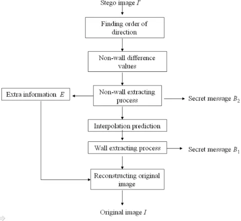
In the extraction, the decoder will exactly extract the embedded secret message B 1 and B 2

from stego image I with side information. In addition, the original image is reconstructed without any distortion. Figure 8 provides the flowchart of data extracting algorithm.

================================Figure 8================================

Figure 8. Flowchart of data extracting algorithm

The detail data extracting algorithm is presented as follows.

Data extracting algorithm

Input: Stego image I, side information Output: Original image I, secret message B

Step 1: Classify all pixels of stego image as wall pixels and non-wall pixels with the same

rule as that used in embedding procedure.

Step 2: Firstly, for non-wall pixels, the processed order of pixels is arranged based on the direction order, as shown in Figure 6.

Step 3: According to the processed order of pixels, calculate the non-wall difference values.

For the current being processed pixel, since its parent pixel must be always processed before it, i.e., its parent pixel has been recovered, then the difference value of the current pixel P k is calculated based on its recovered parent pixel with Equation (14), where k > 1. Since the start pixel in stego image, i.e., k = 1, is reserved from the embedding procedure, it is directly used to reconstruct the original image.

d _k (i, j )=P _k (i, j )−( P _k (i , j)) ^reco _pare , (14) where ( P _k ( i , j)) ^reco _pare represents, for the current being processed pixel P k at coordinate (i, j), the value of its parent pixel of the reconstructed original image.

Step 4: Each secret bit b of message M is alternatively extracted by using Equation (15), and the recovered pixel P reco at coordinate (i, j) is reconstructed by applying Equation (16).

0 if d

( i , j )= Hd

or Hd

, 1 if d

( i , j )= Hd

+1 or Hd

−1 .

¿ b =¿ ^{ ¿ ¿ ¿

¿ (15)

P _k (i , j )−1 , if Hd ₁ +1 ≤d _k ( i , j )≤Zd ₁ , P _k ( i , j )+ 1 if Zd ₂ ≤d _k (i , j )≤ Hd ₂ −1,

P _k ( i , j ) otherwise .

¿

P _reco (i , j )=¿ ^{ ¿ ^{ ¿ ¿ ¿

¿ (16)

Step 5: For wall pixels, the interpolation prediction method is used to generate the interpolation value P pre of each wall pixel P by two pairs of neighboring, restored, non-wall pixels along orthogonal direction of ^{0 } and ^{90 } . Then, interpolation error e is computed by subtracting the corresponding interpolation value P pre from the wall pixel P at coordinate (i, j), i.e., e(i, j)

= P(i, j) – P pre (i, j).

Step 6: Alternatively, each secret bit b of message B 1 is extracted by using Equation (17), and the recovered pixel P reco at coordinate (i, j) is reconstructed by applying Equation (18).

0 if e ( i , j )= He

or He

, 1 if e( i , j )= He

+1 or He

−1 .

b=¿ ¿ { ¿ ¿ ¿

¿ (17)

P ( i , j )−1 , if He ₁ + 1 ≤e (i , j )≤Ze ₁ , P ( i , j )+1 if Ze ₂ ≤ e ( i , j )≤ He ₂ −1,

P ( i , j ) otherwise .

¿

P _reco (i , j )=¿ { ¿ { ¿ ¿ ¿

¿ (18)

After above six steps are processed completely, the secret messages B 1 and M are extracted correctly from stego image and a secondary image can be obtained. If overflow and underflow occurred, the message M is separated into the extra information E and the secret message B 2 . Therefore, the original image can be exactly recovered from the secondary image without any distortion based on the extra information E. Otherwise, the entire message M becomes the secret message B 2 , and the secondary image becomes the reconstructed original image. Finally, concatenate B 1 and B 2 to form the secret message B.

3.3. Side information

In the side information, first we use one bit to indicate whether the extra information exists.

Bit 0 represents no extra information was produced in pre-processing step, i.e., the size of extra information E is 0, while bit 1 represents that the extra information was generated and has been embedded into the non-wall pixels. Next, another two bits are used to record . For He 1 , He 2 , Hd 1 , Hd 2 , since they are very close to 0 or exactly 0, we use two bits to record the value of each, and one bit to indicate the sign of each. Therefore, three bits are sufficient to record each of these peak pints. For Ze 1 , Ze 2 , Zd 1 , Zd 2 , their values are always smaller than 128 and larger than -128. Thus, seven bits are used to record each of them. Consequently, the size of side information for single layer embedding is 1+2+4×3+4×7=43 bits . We arrange the structure of the side information as shown in Figure 9.

=================================Figure 9===============================

Figure 9. Side information

Since our scheme is reversible, it can be used to implement multilayer embedding to achieve

the requirement for larger payload. Then, the corresponding side information generated from the

previous embedding layer can be concatenated with the to-be-embedded secret message M as

shown in Figure 10, and we may embed them together into non-wall pixels of the current

embedding layer. Certainly, the size of side information must be adjusted accordingly because the

pixels may be modified by more than one grayscale value in multilayer embedding. Through the

simulation of a lot of experiments, it is enough that, for each embedding layer, eight bits are used

to record zero point, Ze 1 , Ze 2 , Zd 1 , Zd 2 , and five bits are used to record peak point, He 1 , He 2 , Hd 1 ,

Hd 2 , respectively. Therefore, 55-bits side information of the previous embedding layer will be

inserted into the current embedding layer with secret message M.

===============================Figure 10================================

Figure 10. Structure of to-be-embedded message into non-wall pixels for multilayer embedding

The more embedding layers are used, the worse the image quality will become. Hence, to guarantee the visual quality of the stego image to be accepted, an additional four bits are added to the side information for the last layer to record the number of embedding layers. Therefore, for the multilayer embedding, the size of side information for the last layer is 1+2+4×5+4×8+4=59 bits. The decoder can use the received 59-bits side information of the last embedding layer to extract the secret data and reconstruct the original image. Moreover, the decoder simply can identify single layer or multilayer embedding according to the size of the received side information without any other information.

4. Experimental results

In order to demonstrate the superiority of our proposed scheme over some existing schemes, some experimental results are shown in this section. Six standard grayscale images, from complex to smooth, were selected as the testing images in the resolution of 512×512 pixels as shown in Figure 11. In our experiments, we took a pseudo-random bit generator to produce the secret bits, and adopted peak signal to noise ratio (PSNR) and embedding payload (bits or bpp) as metrics to evaluate the image quality and embedding capacity, respectively.

================================Figure 11===============================

Figure 11. Six 512×512 grayscale testing images

For single layer embedding, since our proposed scheme basically modifies each pixel value at

most by one, the PSNR value of stego image is larger than 10×log ² (255 ² / 1)=48 .13 dB . Table

2 shows the comparison results of maximum embedding capacity and corresponding PSNR

between our proposed scheme and Kim et al.’s [4], Li et al.’s [14], Tsai et al.’s [15] and Luo et

al.’s [18] schemes for six testing images. In Kim et al.’s schemes, four sub-sampled images were

implemented and the embedding level EL was set to 1 to get similar embedding payload as our

proposed scheme. In Tsai et al.’s scheme, the block size was set to 3×3 as suggested in their

paper. In Luo et al.’s scheme, the block size and the embedding level EL were set to ^4×4 and 0,

respectively. In Li et al.’s scheme, we used the APD 2 scheme as described in their paper. In our proposed scheme, we set  to 1, 2 and 3, respectively.

Table 2. Comparison results in terms of capacity and PSNR value for six testing images

===============================Table 2=================================

As shown in Table 2, the embedding performance of the proposed scheme outperforms Kim et al.’s, Luo et al.’s and Li et al.’s schemes. Since three peak bins were used to embed secret message, the payload of the proposed scheme with  = 2 or 3 for Zelda and Barbara was lower than that of Kim et al.’s scheme. However, the average PSNR value of ours was 4.55dB greater than their scheme. If the embedding level of Kim et al.’s scheme was set to 0, the capacity of their scheme was similar to that of Tsai et al.’s scheme. Since the reference pixels were not designed to carry secret data in Tsai et al.’s scheme, it can obtain better image quality. Therefore, to achieve similar PSNR, we embedded no secret data into wall pixels with  = 2. According to the experimental results shown in the last line of Table 2, our scheme can gain the advantages of embedding payload and image quality over Tsai et al.’s scheme.

Figures 12(a)-(f) reveal that the multilayer embedding performance of the proposed scheme outperforms other schemes. Basically, for the six testing images, the top curve is the proposed scheme, i.e., at the same PSNR value, the embedding capacity of the proposed scheme is larger than those of other schemes, and in the same way, when the same payload are embedded, the proposed scheme also has lower image distortion than those of other schemes, especially than Kim et al.’s and Luo et al.’s schemes. Moreover, Figure 12 shows that the proposed scheme obtains larger payload with lower image distortion than Li et al.’s scheme, especially for Barbara. For Tsai et al.’s and Li et al.’s schemes, which achieve large capacity through multilayer embedding, their curves outperform each other over the different images. For example, for Lena, Baboon and Peppers, Li et al.’s scheme always performs better than Tsai et al.’s scheme. On the contrary, for Zelda, Barbara and Airplane, Tsai et al.’s scheme has the advantage over Li et al.’s scheme with the increase of embedding layer. Therefore, Figure 12 also indicates that the proposed scheme is more stable than other schemes for difference images.

================================Figure 12===============================

Figure 12. Performance evaluation of multilayer embedding over six standard testing images

5. Conclusions

In this paper, a novel, reversible, data hiding scheme based on histogram shifting is proposed for high quality images. To achieve larger embedding capacity and higher image quality, we classify all pixels as wall pixels and non-wall pixels. The secret message are respectively embedded into wall pixels based on the interpolation errors, and into non-wall pixels according to the difference values between they and their corresponding parent pixels, which are defined by the direction order. By applying histogram shifting to these interpolation errors and difference values, we not only guarantee the high image quality but also provide the large embedding capacity.

According to the experimental results, the proposed reversible scheme achieves larger payload and better visual quality than those of some schemes for single layer embedding and multilayer embedding. In addition, the performance of the proposed scheme is more stable for different images.

References

[1] J. S. Pan, M. T. Sung, H. C. Huang, B. Y. Liao, Robust VQ-based digital watermarking for the memory less binary symmetric channel, Proceedings of 2004 International Symposium on Circuits and Systems(ISCAS04), vol. 5 ,2004, pp. V-580 - V-583.

[2] M. Iwata, K. Miyake, A. Shiozaki, Digital steganography utilizing features of JPEG images, IEICE Transactions on Fundamentals of Electronics, Communications and Computer Sciences, E87-A (4) (2004) 929–936.

[3] J. Mielikainen, LSB matching revisited, IEEE Signal Processing Letters, 13 (5) (2006) 285–

287.

[4] K. S. Kim, M. J Lee, H. Y. Lee, H. K. Lee, Reversible data hiding exploiting spatial correlation between sub-sampled images, Pattern Recognition, 42 (11) (2009) 3083-3096.

[5] C. C. Chang, T. D. Kieu, Y. C. Chou, Reversible information hiding for VQ indices based on locally adaptive coding, Journal of Visual Communication and Image Representation, 20 (1) (2009) 57–64.

[6] B. Yang, M. Schumucker, W. Funk, C. Brush, S. Sun, Integer DCT-based reversible

watermarking for images using compounding technique, Proceedings of SPIE, Security,

Steganography and Watermarking of Multimedia Contents, San Jose, CA, vol. 5306, 2004,

pp. 405-415.

[7] G. Xuan, Q. Yao, C. Yang, J. Gao, P. Chai, Y. Q. Shi, and Z. Ni, Lossless data hiding using histogram shifting method based on integer wavelets, Proceedings of International Workshop on Digital Watermarking, Lecture Notes in Computer Science, 4283, 2006, pp. 323-332.

[8] C. C. Chang, C. Y. Lin, Y. H. Fan, Lossless data hiding for color images based on block truncation coding, Pattern Recognition, 41 (7) (2008) 2347-2357.

[9] J. Tian, Reversible data hiding using difference expansion, IEEE Transactions on Circuits and Systems for Video Technology, 13 (8) (2003) 890-896.

[10] C. C. Chang and T. C. Lu, A difference expansion oriented data hiding scheme for restoring the original host images, The Journal of Systems and Software, 79 (12) (2006) 1754-1766.

[11] C. C. Chang, T. D. Kieu, W. C. Wu, A lossless data embedding technique by joint neighboring coding, Pattern Recognition, 42 (7) (2009) 1597–1603.

[12] C. C. Lee, H. C. Wu, C. S. Tsai, Y. P. Chu, Adaptive lossless steganographic scheme with centralized difference expansion, Pattern Recognition, 41 (6) (2008) 2097-2106.

[13] C. C. Lin, N. L. Hsueh, A lossless data hiding scheme based on three-pixel block differences, Pattern Recognition, 41 (4) 2008 1415-1425.

[14] Y. C. Li, C. M. Yeh, C. C. Chang, Data hiding based on the similarity between neighboring pixels with reversibility, Digital Signal Processing, 20 (4) 2010 1116-1128.

[15] P. Tsai, Y. C. Hu, H. L. Yeh, Reversible image hiding scheme using predictive coding and histogram shifting, Signal Processing, 89 (6) 2009 1129-1143.

[16] Z. Ni, Y. Q. Shi, N. Ansari, W. Su, Reversible data hiding, IEEE Transactions on Circuits and Systems for Video Technology, 16 (3) 2006 354-362.

[17] Z. Zhao, H. Luo, Z. M. Lu, J. S. Pan, Reversible data hiding based on multilevel histogram modification and sequential recovery, International Journal of Electronics and Communications, 2011, doi: 10.1016/j.aeue.2011.01.014.

[18] H. Luo, F. X. Yu, H. chen, Z. L. Huang, H. Li, P. H. Wang, Reversible data hiding based on block median preservation, Information Sciences, 181 (2) (2011) 308-328.

[19] L. Luo, Z. Chen, M. Chen, X. Zeng, Z. Xiong Reversible image watermarking using

interpolation technique, IEEE Transactions on Information Forensics and Security, 5 (1)

(2011) 187-193.

Figure 1. Flowchart of data embedding algorithm

Table 1. Block classification based on median

Block Type Conditions

Type I n 0 = 1

Type II

Type II-1 n 0 ≥ 2, n l = n r

Type II-2 n 0 ≥ 2, n l < n r

Type II-3 n 0 ≥ 2, n l > n r

Figure 2. Pixel classification

Figure 3. Flowchart of data embedding algorithm

Figure 4. Histogram of interpolation errors of wall-pixels

Figure 5. Shifted histogram of interpolation errors of wall-pixels

Figure 6. Direction order

Figure 7. Processed order of pixels based on direction order

Figure 8. Flowchart of data extracting algorithm

Figure 9. Side information

Figure 10. Structure of to-be-embedded message into non-wall pixels for multilayer embedding

Table 2. Comparison results in terms of capacity and PSNR value for six testing images

Scheme Metric Lena Airplane Baboon Peppers Zelda Barbara

Kim et al.’s scheme Capacity(bits) 61832 81173 20965 59707 63399 38289

PSNR(dB) 44.20 44.55 43.63 44.16 44.20 43.85

Luo et al.’s scheme Capacity(bits) 29813 44786 9522 28271 27372 17555

PSNR(dB) 48.68 48.83 48.50 48.67 48.65 48.56

Tsai et al.’s scheme Capacity(bits) 47912 64996 15820 45496 48608 29398

PSNR(dB) 49.06 49.24 48.73 49.03 49.06 48.86

(a) Lena (b) Airplane (c) Baboon

(d) Peppers (e) Barbara (f) Zelda

Figure 11. Six 512×512 grayscale testing images

Li et al.’s scheme Capacity(bits) 60817 79295 23946 62255 54460 33890

PSNR(dB) 48.67 48.75 48.33 48.68 48.60 48.42

Proposed scheme with  = 1

Capacity(bits) 71191 87301 24855 66934 69635 40383

PSNR(dB) 48.80 48.98 48.50 48.75 48.76 48.49

Proposed scheme with  = 2

Capacity(bits) 65462 83022 24250 64228 61277 36731

PSNR(dB) 48.75 48.92 48.38 48.72 48.67 48.45

Proposed scheme with  = 3

Capacity(bits) 63365 81533 24315 63558 58247 35367

PSNR(dB) 48.72 48.90 48.39 48.74 48.65 48.44

Proposed scheme without wall-pixels( = 2)

Capacity(bits) 53945 70681 20592 54262 50170 30460

PSNR(dB) 49.20 49.40 48.87 49.21 49.18 48.97

0 0.2 0.4 0.6 0.8 1 1.2 1.4 25

30 35 40 45 50

Payload (bpp)

PS N R ( dB )

Kim et al.'s Scheme Luo et al.'s Scheme Li et al.'s Scheme Tsai et al.'s Scheme Proposed Scheme

0 0.2 0.4 0.6 0.8 1 1.2 1.4

30 32 34 36 38 40 42 44 46 48 50

Payload (bpp)

PS N R ( dB )

Kim et al.'s Scheme Luo et al.'s Scheme Li et al.'s Scheme Tsai et al.'s Scheme Proposed Scheme

(a) Lena (b) Airplane

0 0.1 0.2 0.3 0.4 0.5 0.6 0.7

25 30 35 40 45 50

Payload (bpp)

PS N R ( dB )

Kim et al.'s Scheme Luo et al.'s Scheme Li et al.'s Scheme Tsai et al.'s Scheme Proposed Scheme

0 0.2 0.4 0.6 0.8 1 1.2 1.4

30 32 34 36 38 40 42 44 46 48 50

Payload (bpp)

PS N R ( dB )

Kim et al.'s Scheme Luo et al.'s Scheme Li et al.'s Scheme Tsai et al.'s Scheme Proposed Scheme

(c) Baboon (d) Peppers

0 0.2 0.4 0.6 0.8 1 1.2 1.4

30 32 34 36 38 40 42 44 46 48 50

Payload (bpp)

PS N R ( dB )

Kim et al.'s Scheme Luo et al.'s Scheme Li et al.'s Scheme Tsai et al.'s Scheme Proposed Scheme

0 0.1 0.2 0.3 0.4 0.5 0.6 0.7 0.8

25 30 35 40 45 50

Payload (bpp)

PS N R ( dB )

Kim et al.'s Scheme Luo et al.'s Scheme Li et al.'s Scheme Tsai et al.'s Scheme Proposed Scheme

(e) Zelda (f) Barbara

Figure 12. Performance evaluation of multilayer embedding over six standard testing images