Proceedings of the ASME 2020 39th International Conference on Ocean, Offshore and Arctic Engineering OMAE2020 August 3-7, 2020, Virtual, Online
OMAE2020-18233
THE DEVELOPMENT OF AN ANALYTICAL WAKE MODEL FOR THE FLOW-FIELD ASSESSMENT OF OFFSHORE WIND FARMS
Bryan Nelson, Tsung-yueh Lin CR Classification Society
Taipei, Taiwan
ABSTRACT
There are several analytical wake models in current use which have, over the years, been shown to adequately predict the flow- fields through large wind farms. However, many of these wake models are based on momentum theory, which assumes no frictional drag and a non-rotating wake, the effects of which may not be neglected at non-optimum operating conditions. To address these shortcomings, we are developing an analytical wake model, derived from unsteady, 3D, full-rotor CFD simulations of the flow field behind a single wind turbine for its full range of operating conditions. The proposed model will be validated against site data from the literature, as well as against data predicted using commercial tools. This study is part of the development of a framework for the real-time assessment of the wind farm power generation, together with the wind/wave loads acting on the individual wind turbines and their support structures, within a large offshore wind farm.
Keywords: wind farm, wake effects, flow field, energy yield
INTRODUCTION
In order to increase energy security and decrease carbon emissions, Taiwan’s Ministry of Economic Affairs’ (MOEA) has been aggressively promoting the development of a localised renewable energy industry. Due to the island nation’s world- class wind resources, the MOEA has focused their attention on the development of their local wind energy industry, recently raising their 2025 installed offshore capacity target to 5.7 GW, with an estimated total investment of around NT$ 1 trillion [1].
These offshore wind farms will comprise dozens if not hundreds of wind turbines working together to generate electricity.
Grouping wind turbines together in this way allows for a reduced levelised cost of electricity (LCOE), but also introduces new design problems, such as inter-turbine flow interactions, or
“wake effects”, which are known to reduce the wind farms’ total output power, while simultaneously increasing the fatigue loading of the downstream wind turbines.
The planning, development, and financing of large-scale wind energy projects, such as the MOEA’s “Thousand Wind Turbines” project, necessitate accurate, reliable tools for wind energy yield and load assessments so as to reduce risk and maximise return on investment. These energy yield assessments are complicated by so-called wake effects, such as wake shadowing and wake meandering [2]. Such wake effects severely reduce the amount of wind energy available to those wind turbines located in the wakes of upstream turbines, such that the total power production of the wind farm is diminished, while the increased turbulence in the wakes also gives rise to increased load fluctuations (fatigue loading) [3].
JENSEN’S WAKE MODEL
One of the earliest wake models still in common use is that proposed by N.O. Jensen in 1983 [4]. It is a very simple model, assuming a linearly expanding wake, with a velocity deficit that is a function of the distance behind the rotor 𝑥 and the wind turbine’s thrust coefficient 𝐶𝑇. The diameter of the wake 𝐷𝑤 at a downstream distance 𝑥 is given by:
𝐷𝑤= 𝐷(1 + 2𝑘𝑠) (1)
and the velocity in the (fully developed) wake is given by
𝑢 = 𝑈∞[1 −1 − √1 − 𝐶𝑇
(1 + 2𝑘𝑠)2 ] (2)
where 𝐷 is the rotor diameter, 𝑈∞ is the far-field velocity, 𝑠 = 𝑥/𝐷 is the non-dimensionalised distance behind the rotor, and the Wake Decay Constant is set as k = 0.04, which corresponds to the case of low atmospheric turbulence (TI = 8%), often referred to as offshore conditions [5]. Despite its simplicity, the Jensen wake model has been shown to be very reliable [6], and is the default model adopted by Risø DTU’s WAsP, GH’s WindFarmer, UL’s OpenWind, and EMD’s WindPRO, to name a few.
For the case of multiple wakes, the present study employs the
“sum of squares of velocity deficits” wake combination model proposed by Katic [7]:
(1 − 𝑢𝑗
𝑈∞
)
2
= ∑ (1 −𝑢𝑗𝑖
𝑢𝑖
)
2𝐴shadow,𝑖 𝐴0 𝑁
𝑖
(3)
where 𝑢𝑗 is the wind speed at turbine 𝑗 due to all upstream turbines, 𝑢𝑖 is the wind speed at upstream turbine 𝑖, 𝑢𝑗𝑖 is the wind speed at turbine 𝑗 due to the wake of turbine 𝑖, and the summation is taken over the 𝑁 turbines upstream of turbine 𝑗.
For the case of partially overlapped wakes, the velocity deficit is weighted by the fraction of the overlapping area 𝐴shadow to the rotor area of the down-stream turbine 𝐴0 . For the standard Jensen model, where the transverse velocity distribution in the wake is uniform, 𝐴shadow may be calculated analytically [8].
However, it has been shown [9] that a Gaussian or cosine profile better represents the actual velocity distribution in the downstream wake (as illustrated in Figure 1). To allow us to incorporate different velocity distributions into our wake model, we decided to calculate 𝐴shadow numerically, by discretising the rotor/wake plane onto a Cartesian grid (Figure 2).
The cosine velocity distribution, achieved by Equation (4) [7], assumes the following:
• The wake diameter is equal to that given by the standard Jensen wake model (Equation 1);
• The mass flux 𝑄, calculated by integrating the wind speed in the transverse (cross wind) plane (Equation 5), is equivalent to that given by the standard Jensen model.
𝑢′(𝑟) = (𝑈∞− 𝑢)cos(𝜋 𝑟 𝑟𝑤
+ 𝜋) + 𝑢 (4)
𝑄 = ∫ 𝑢′𝑑𝑟
𝑟𝑤 0
(5)
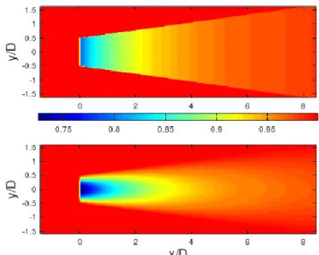
where 𝑢′(𝑟) is the velocity distribution in the transverse plane, 𝑟 is the radial distance from the centre of the wake (𝑟 < 𝑟𝑤), and 𝑟𝑤 is the radius of the wake at downstream location 𝑥 (Equation 1). The hub-height flow fields predicted by the standard and cosine Jensen wake models are shown in Figure 3.
Figure 1. Wind speed distribution in a turbine wake at 5D downwind (Wind tunnel data obtained from [10])
Figure 2. Wake-overlap area 𝐴shadow calculated by discretisation of rotor/wake plane (coloured by cosine velocity distribution)
Figure 3. Velocity distribution behind a wind turbine, as predicted by the standard (top) and cosine (bottom) Jensen wake models
PROPOSED WAKE MODEL
Despite its impressive track record, Jensen’s model (like all so- called kinematic models) suffers from two significant shortcomings, both of which stem from its basis in one- dimensional momentum theory. The first of these limitations is that 1-D momentum theory, and consequently Jensen’s wake model, is not valid for 𝐶𝑇> 1, as may be seen from Equation 2.
This condition, though not overly common, may be observed at low wind speeds for a non-negligible number of commercial wind turbines [11]. The second limitation stems from two of the 1-D momentum theory’s key assumptions, namely (1) no frictional drag, and (2) a non-rotating wake. While these assumptions may be appropriate at optimum operating conditions (i.e. around rated wind speed), the effects of frictional drag and the rotating wake may not be neglected at high tip- speed-ratios (low-to-negative angles of attack) and at low tip- speed-ratios, where the blades are pitched to maintain constant power and to reduce aerodynamic loading.
In order to overcome the above-mentioned limitations, we are currently developing a new analytical wake model which focuses on the relationship between the velocity deficit in the wake and the wind turbine’s tip-speed-ratio. To this end, we have performed a number of unsteady 3D full-rotor CFD simulations, using the commercial RANS-based code STAR-CCM+. The modelled domain is illustrated in Figure 4, and a view of the surface mesh on the wind turbine hub and blades is shown in Figure 5. The computational domain has a diameter of four rotor diameters (4D), and extends two rotor diameters (2D) upstream, and eight rotor diameters (8D) downstream.
The target wind turbine for this study was the NREL 5 MW reference turbine, and our CFD results were validated against the power and thrust coefficients provided in the target wind turbine’s documentation [12]. Figure 6 shows that there is excellent agreement between the two sets of power and thrust coefficients, giving us confidence that our mesh resolution near the wind turbine is sufficiently fine. However, in order to assess the validity of the results throughout the downstream wake region, we performed a mesh independence assessment, running a number of different mesh configurations, some of which are shown in Figure 7, together with their respective mesh counts, and then parametrically analysing the wake profiles (circumferentially-averaged velocity distributions) at several downstream locations (Figure 8).
The results of the mesh independence assessment clearly show that finer mesh resolutions produced more pronounced wake profiles, with greater velocity deficits, higher wake-core velocities, as well as sharper transitions from free-stream velocity to wake velocities. On the other hand, our coarse mesh, Mesh A, significantly underpredicted the velocity deficit in the far-wake, while overpredicting the wake expansion, i.e. the diameter of the wake profile. Interestingly, it appears that extending the very fine volumetric control region to around 4D
downstream (Mesh D) produces very similar results to those attained by extending the volumetric control throughout the computational domain.
Figure 4. Computational domain forunsteady 3D full CFD simulation
Figure 5. Surface mesh on the wind turbine hub and blades
Figure 6. Validation of CFD results for Power and Thrust curves
Mesh A (7 million cells)
Mesh B (9 million cells)
Mesh C (12 million cells)
Mesh D (20 million cells)
Mesh E (32 million cells)
Figure 7. Mesh configurations for mesh independence assessment (Not pictured: Mesh F, which resembles Mesh E, but has 50M cells)
(a) 2D
(b) 4D
(c) 6D
(d) 8D
Figure 8. Wake profiles (circumferentially-averaged velocity distribution) for mesh independence assessment
To more quantitatively assess the mesh independence, we compared the deficit of volumetric flow rate in the wake Δ𝑄, (Equation 6) which was computed by radially integrating the wake velocity deficit Δ𝑢 = 𝑈∞− 𝑢𝑤. These results, shown in Figure 9, are clearly seen to converge in meshes D, E, and F. It was therefore decided to adopt Mesh D for the full range of operating conditions.
Δ𝑄 = ∫ Δ𝑢
𝑟𝑤 0
𝑑𝑟 (6)
Figure 9. Normalised deficit of volumetric flow rate in the wake Δ𝑄 The next step was to parameterise the wake profile, and find a curve to fit the wake’s geometric features while also matching its volumetric flow rate deficit Δ𝑄 . First, we min-max normalised the velocity, and then measured the abscissae (radial distance 𝑟 ) and ordinates (min-max normalised velocity 𝑢̂ ) of the minimum velocity in the wake (i.e. maximum velocity deficit) and the maximum velocity outside the wake region. It was found that the wake profile was best described by the Gumbel distribution:
𝑢(𝑟) =𝑐
𝛽𝑒−(𝑧+𝑒−𝑧) (5)
where 𝑧 = (𝑥 − 𝜇)/𝛽 , and 𝛽 and 𝜇 are, respectively, the location and scale parameters, and 𝑐 is introduced to improve the curve fit. The parameters 𝛽, 𝜇, and 𝑐 may be calculated at downstream distance 𝐷 by using Equations 6, which were determined by linear regression of the Gumbel curve fit results.
𝛽 = 0.173 − 0.005 𝐷
𝜇 = 0.666 + 0.019 𝐷 (6)
𝑐 = 0.491 − 0.015 𝐷
Figure 10 shows our CFD-determined wake profiles (solid lines), together with the fitted Gumbel curves (dashed lines).
Figure 10. Normalised wake profile with fitted Gumbel curves
CASE STUDY 1: FUHAI OFFSHORE WIND FARM To verify that our standard Jensen model (Equation 2) runs as intended, we first compared results with those computed using the Wind Atlas Analysis and Application Program (WAsP) [13], which also employs the standard Jensen model. In this way, we were able to ensure consistency between our two compared tools in terms of input meteorological data and the locations and specifications of the individual wind turbines.
The target wind farm for this test was the FuHai Offshore Wind Farm, currently under construction off Taiwan’s west coast. The FuHai wind farm proposal initially consisted of 29 Siemens SWT-4.0-120 wind turbines. The adopted power and thrust coefficient curves and the locations of the 29 wind turbines are shown in Figures 11 and 12, respectively.
The standard Jensen wake model was run for the full range of operational wind speeds, from 3.5 m/s to 32.5 m/s, with 1 m/s steps, and for the full range of wind directions, from –0.5° to 359.5°, with 1° steps. The directional results were then binned into the eight principal wind directions, or sectors.
The energy yield assessment was based on pre-construction meteorological data collected at the site over the course of one year, from the 1st of January to the 31st of December, 2008. The WAsP energy yield prediction was based on sector-wise probability distributions of the wind speed, specifically two- parameter Weibull distributions:
𝑓(𝑢) =𝑘 𝐴(𝑢
𝐴)
𝑘−1
𝑒−(𝑢/𝐴)𝑘 (7)
where 𝑓 is the probability of occurrence of a given wind speed 𝑢, and 𝑘 and 𝐴 are, respectively, the shape and scale factors of the probability distribution function (PDF). The Weibull shape
and scale parameters are estimated by curve-fitting Weibull PDFs to sector-wise histograms of the wind speed data. The sector wise Weibull parameters are listed in Table 1.
Figure 11. Adopted wind turbine power/thrust curves
Figure 12. Wind turbine locations in FuHai OWF
Table 1 Meteorological data Wind
direction
Weibull parameters Frequency A k [%]
N 11.24 1.955 17.3
NNE 12.29 1.963 43.1
ENE 7.54 1.221 5.1
E 4.09 1.033 1.5
ESE 4.10 1.131 2
SSE 4.54 1.143 5.4
S 5.28 1.557 8.4
SSW 7.25 1.814 5.9
WSW 6.97 1.732 4.9
W 6.21 1.893 2.7
WNW 5.33 1.17 1.6
NNW 5.37 1.186 2.3
All 9.52 1.549 100
The energy yield results predicted by our standard Jensen wake model, for each of the wind turbines in the FuHai Offshore Wind Farm, are plotted in Figure 13, together with the results predicted
by WAsP. The results have been normalised by the wind farm’s gross (no losses) annual energy yield divided by the number of turbines. To investigate the accuracy of WAsP’s Weibull PDF curve fitting procedure, we also assessed the energy yield based on the discrete meteorological site data, which is also shown in Figure 13. The total annual energy yield results for the FuHai OWF are summarised in Table 2.
Figure 13 shows that there is excellent agreement between the energy yield results predicted by our standard Jensen wake model, for each of the wind turbines in the FuHai Offshore Wind Farm, and those predicted by WAsP, with a maximum discrepancy of less than 1%. For the most part, the per turbine results based on the discrete meteorological site data show even closer correlation with the WAsP results, except for the farthest downstream turbines, WT #26 to WT #28, for which the discrepancy slightly exceeds 2%.
Figure 13. Energy yield results for FuHai OWF (per WT)
Table 2 Energy yield for FuHai OWF (Total)
Model Total energy
[MWh/y] Error
[%] Wake losses [%]
WAsP 424072.1 – 7.2
Jensen (Weibull) 423841.1 0.05 7.2 Jensen (site) 426681.0 0.62 6.6
In terms of total annual energy yield, there is less than 1%
discrepancy between our Jensen model results and those from WAsP, with our results derived from WAsP’s Weibull PDFs showing just 0.5% discrepancy. The reasons for these discrepancies are still being evaluated, but are most likely due to rounding errors, such as in the adopted Weibull parameters, and possibly due to differences in the binning criteria.
On the whole, the wake losses for this relatively small wind farm were fairly inconsequential, at around just 7% for the total annual energy yield. In terms of model performance, the authors are satisfied that our standard Jensen model runs as intended, and in the following section, we shall validate our model against SCADA data from a larger wind farm.
CASE STUDY 2: HORNS REV I
To investigate the effects of our two tested velocity profiles, we compared the results of our standard and cosine Jensen wake models with operational data recorded by the Supervisory Control and Data Acquisition (SCADA) system of a large scale wind farm.
The target wind farm for this test was Horns Rev I, located in the North Sea, approximately 14 km off Denmark’s west coast.
Horns Rev was the world’s first large scale offshore wind farm, consisting of 80 Vestas V80-2.0 MW turbines, for a total installed capacity of 160 MW. Construction was completed in 2002, and operational data recorded by the wind farm’s SCADA system has since been utilised for several wake model benchmarking studies [14, 15, 16, 17]. The adopted power and thrust coefficient curves for the Vestas wind turbines and the wind farm layout are illustrated in Figures 14 and 15, respectively.
As discussed in the literature, there is a significant degree of uncertainty in the SCADA data, due to such factors as yaw misalignment of the reference turbine, spatial variability of the wind direction within the wind farm, and wind direction averaging period. It is usually found that this directional uncertainty may be reduced by binning the directional data in sufficiently wide bins [17].
The present study adopted the SCADA data for a westerly wind, i.e. 270° ± 15°. For our test, we took the average of several simulations performed for the same 30° range of “westerly”
winds, with 1° steps. The results of this validation test case are shown in Figure 16, which also includes simulated results predicted by Wu et al. [18] using large eddy simulations (LES).
The results in Figure 16 are those of the 10 wind turbines in Row D (Figure 15), such that WT #1 is upwind, and does not suffer any wake losses. Accordingly, the energy yields of the nine downwind turbines have been normalised against WT #1. The total output power results for the Horns Rev I Offshore Wind Farm are summarised in Table 3.
Figure 16 shows how the standard Jensen model overestimates the wake losses for the first few downstream turbines, particularly WT #2 to WT #6. For these same few wind turbines, the cosine Jensen model shows excellent agreement with the SCADA site data. However, from WT #7 onwards, both of the Jensen models level off to a constant output, while the site data shows that the output power of the downwind turbines continues to fall. By comparison, the LES data captures the trend fairly well, but is shown to overestimate the output power at all of the downwind turbines.
Figure 14. Adopted Vesta V-80 turbine power/thrust curves
Figure 15. Horns Rev I wind farm layout [14]
Figure 16. Energy yield results for Horns Rev I OWF (per WT), normalised against WT #1, for wind direction 270° ± 15°
Table 3 Results for Horns Rev I Offshore Wind Farm
Model Total energy
(normalised) Error [%]
SCADA 0.723 –
LES 0.769 6.5
Jensen (standard) 0.712 1.4 Jensen (cosine) 0.745 3.1
* Please note that the results of our proposed wake model are still pending.
CONCLUSION
To address the shortcomings of the many analytical wake models which are based on momentum theory, we are currently developing a wake model, derived from unsteady, 3D, full-rotor CFD simulations of the flow field behind a single wind turbine for its full range of operating conditions. This paper describes our CFD model setup, and the parameterisation of our CFD model results, and also describes the two existing wake models against which our analytical model will be compared. In the preliminary stage of this study, we performed several verification tests for the adopted Jensen wake model. The standard Jensen model was shown to correlate extremely well with that employed by the Wind Atlas Analysis and Application Program (WAsP), and comparing two different velocity profiles with SCADA data from a large scale wind farm showed excellent agreement with the SCADA data for the first few downstream turbines, but both wake profiles were shown to underpredict the wake losses in wind turbines farther downstream. Results from our RANS- based parameterised model of the wake profile, which will next be included in our wind farm analysis tool, are to be compared with our Jensen model results.
ACKNOWLEDGEMENTS
This research was partially supported by the BSMI Project:
1D171080121-31.
REFERENCES
[1] Taiwan Executive Yuan, Four-year Wind Power Promotion Plan,https://english.ey.gov.tw/News3/9E5540D592A5FECD/d603 a1bf-9963-4e53-a92b-e6520a3d93ff
[2] The Wake Effect: Impacting turbine siting agreements. North American Clean Energy.
http://www.nacleanenergy.com/articles/15348/the-wake-effect- impacting-turbine-siting-agreements
[3] N.O. Jensen, “A note on wind generator interaction”, Roskilde:
Risø National Laboratory. Risø-M, No.2411, 1983
[4] B. Nelson, Y. Quéméner, T-Y Lin, “Effects of Wake Meander on Fatigue Lives of Offshore Wind Turbine Jacket Support Structures”, 2018 Taiwan Wind Energy Association Conference, Tainan, Taiwan
[5] van Heemst, J.W., Improving the Jensen and Larsen Wake Deficit Models. Using a Free-Wake Vortex Ring Model to Simulate the Near-Wake. MSc Thesis. TUDelft. 2015
[6] D.J. Renkema, “Validation of wind turbine wake models. Using wind farm data and wind tunnel measurements”, MSc Thesis, TUDelft, Netherlands (2007)
[7] I. Katic, J. Højstrup, N.O. Jensen, “A simple model for cluster efficiency”, European Wind Energy Association Conference and Exhibition, 7-9 October 1986, Rome, Italy, 1986.
[8] F. González-Longatt, P. Wall, V. Terzija. Wake effect in wind farm performance: Steady-state and dynamic behavior. Renew. Energy 39(1), 329–338 (2011).
[9] L-L Tian, W-J Zhu, W-Z Shen, N. Zhao, Z-W Shen, “Development and validation of a new two-dimensional wake model for wind turbine wakes”, Journal of Wind Engineering and Industrial Aerodynamics, 137, 90-99 (2015)
[10] W. Schlez, A. Tindal, D. Quarton, “GH Wind Farmer Validation Report”, Garrad Hassan and Partners Ltd, Bristol, 2003.
[11] H-J Gu, J. Wang, Q. Lin, Q. Gong, “Automatic Contour-Based Road Network Designfor Optimized Wind Farm Micrositing”, IEEE Transactions on Sustainable Energy, Vol. 6, No. 1, 2015 [12] J.Jonkman, S. Butterfield, W. Musial, G. Scott, “Definition of a5-
MW Reference Wind Turbine for Offshore System Development”, Technical Report, NREL/TP-500-38060, 2009
[13] WASP User's Manual,
https://www.cs.utexas.edu/~ml/wasp/manual.html
[14] K. Hansen, R. Barthelmie, L. Jensen, A. Sommer, “The impact of turbulence intensity and atmospheric stability on power deficits due to wind turbine wakes at Horns Rev wind farm”, Wind Energy, 15:183e96 (2012)
[15] D.R. VanLuvanee, “Investigation of observed and modeled wake effects at Horns Rev using WindPRO”, Master’s thesis, Technical University of Denmark (2006)
[16] R.J. Barthelmie, K. Hansen, S.T. Frandsen, O. Rathmann, J.G.
Schepers, W. Schlez, J.A. Phillips, K. Rados, A. Zervos, E.S.
Politis, P.K. Chaviaropoulos, “Modelling and measuring flow and wind turbine wakes in large wind farms offshore”, Wind Energy, 12:431e44 (2009)
[17] M. Gaumond, P-E. Réthoré, A. Bechmann, S. Ott, G.C. Larsen, A.
Peña, K.S. Hansen, “Benchmarking of wind turbine wake models in large offshore wind farms”, Proceedings of the Science of making torque from wind conference (2012)
[18] Y-T Wu, F. Porté-Agel, “Modeling turbine wakes and power losses within a wind farm using LES: An application to the Horns Rev offshore wind farm”, Renewable Energy, 75, 945-955 (2015).


![Figure 15. Horns Rev I wind farm layout [14]](https://thumb-ap.123doks.com/thumbv2/9libinfo/9655478.678829/7.918.495.845.424.994/figure-horns-rev-i-wind-farm-layout.webp)

