結合無線定位與雷射測距的適應性室內定位整合系統

行政院國家科學委員會專題研究計畫 成果報告

結合無線定位與雷射測距的適應性室內定位整合系統 研究成果報告(精簡版)

計 畫 類 別 ： 個別型

計 畫 編 號 ： NSC 99-2221-E-011-125-

執 行 期 間 ： 99 年 08 月 01 日至 100 年 07 月 31 日 執 行 單 位 ： 國立臺灣科技大學機械工程系

計 畫 主 持 人 ： 高維文

計畫參與人員： 碩士班研究生-兼任助理人員：陳慶坤 碩士班研究生-兼任助理人員：林敬弦 碩士班研究生-兼任助理人員：余吉祥

報 告 附 件 ： 出席國際會議研究心得報告及發表論文

公 開 資 訊 ： 本計畫可公開查詢

中 華 民 國 100 年 12 月 14 日

中 文 摘 要 ： 本計畫針對目前室內定位常用的兩種方法：無線定位與雷射 測距定位的不同限制進行整合。無線定位常因室內環境的不 確定性造成利用無線信號強度衰減求距離的精度不高，影響 其應用範圍。雷射測距儀搭配室內地標結合 SLAM 演算法則 是智慧型機器人定位的重要方法，但雷射測距儀價格昂貴且 仍有量測範圍及量測誤差的限制。在室內多物件的定位應用 上，本計畫提出主從式的定位架構，以單一同時具備 ZigBee 定位及雷射測距定位能力的主定位器進行擴展式的非線性狀 態估測演算，同時將 ZigBee 的無線信號強度衰減模型參數 視為待估測狀態之一，在主定位器的定位演算過程中逐步修 正無線信號強度衰減模型，提昇 ZigBee 無線定位的精確 性，同時室內其他從屬定位物件則可僅靠修正後的 ZigBee 無線信號強度衰減模型進行定位，以較少較便宜的感測器架 構而達成近似於主定位器整合定位的精度。在定位整合狀態 估測器理論部分，探討不同非線性估測理論應用於本計畫定 位架構下的有效性及定位效能。在應用方面，本計畫成果可 應用於大面積、多載具或具複雜物件並多變動的室內定位應 用環境，達成經濟有效的定位成果。

中文關鍵詞： 室內定位、ZigBee 無線定位、SLAM、卡門濾波、粒子濾波 英 文 摘 要 ： Indoor positioning based on received signal strength

index, or RSSI, is quite popular idea and has been realized by using several wireless networks such as Wi-Fi, Bluetooth, Zigbee, etc. In the

implementations, a signal propagation model is used to characterize the relationship between the measured RSSI and the signal transmitting distance in order to determine the unknown user location with respect to transmitters in known fixed locations. RSSI

measurements have large variations because they are subjected to the deleterious effects of fading or shadowing in dynamic indoor environments and it is difficult to model these effects using fixed

propagation model parameters. Dead-reckoning based systems which detect the user relative motions by various sensors are also popular in indoor

positioning applications. This research integrates the relative displacement information from dead- reckoning systems with a Zigbee RSSI-based

positioning system. Unlike conventional systems, the RSSI model parameters are not consider known or fixed

but are estimated together with the unknown user locations during the motion using both the Extended Kalman filter (EKF) and the Particle filter (PF).

With the capability to dynamically estimate the signal propagation model parameters in changing environments, the positioning accuracy is improved and the integrated system is more suitable to be used in dynamic indoor environments with signal

propagation variations. Both simulation and experiments results are presented to show the

performance of the integrated positioning system in indoor environments.

英文關鍵詞： Indoor positioning, ZigBee Location, SLAM, Kalman filter, Particle filter

行政院國家科學委員會專題研究計畫成果報告

結合無線定位與雷射測距的適應性室內定位整合系統

Adaptive Indoor Positioning System with Wireless Locating and Laser Ranging Techniques

計畫編號：NSC 99-2221-E-011-125 執行期限：99 年 8 月 1 日至 100 年 7 月 31 日

主持人：高維文 國立台灣科技大學機械系 計畫參與人員：陳慶坤、林敬弦、余吉祥

國立台灣科技大學機械系

中文摘要

本計畫針對目前室內定位常用的兩種方 法：無線定位與雷射測距定位的不同限制進 行整合。無線定位常因室內環境的不確定性 造成利用無線信號強度衰減求距離的精度不 高，影響其應用範圍。雷射測距儀搭配室內 地標結合 SLAM 演算法則是智慧型機器人定 位的重要方法，但雷射測距儀價格昂貴且仍 有量測範圍及量測誤差的限制。在室內多物 件的定位應用上，本計畫提出主從式的定位 架構，以單一同時具備 ZigBee 定位及雷射測 距定位能力的主定位器進行擴展式的非線性 狀態估測演算，同時將 ZigBee 的無線信號強 度衰減模型參數視為待估測狀態之一，在主 定位器的定位演算過程中逐步修正無線信號 強度衰減模型，提昇 ZigBee 無線定位的精確 性，同時室內其他從屬定位物件則可僅靠修 正後的 ZigBee 無線信號強度衰減模型進行定 位，以較少較便宜的感測器架構而達成近似 於主定位器整合定位的精度。在定位整合狀 態估測器理論部分，探討不同非線性估測理 論應用於本計畫定位架構下的有效性及定位 效能。在應用方面，本計畫成果可應用於大 面積、多載具或具複雜物件並多變動的室內 定位應用環境，達成經濟有效的定位成果。

關 鍵 詞 ： 室 內 定 位 、 ZigBee 無 線 定 位 、 SLAM、卡門濾波、粒子濾波

ABSTRACT

Indoor positioning based on received signal strength index, or RSSI, is quite popular idea and has been realized by using several wireless networks such as Wi-Fi, Bluetooth, Zigbee, etc. In the implementations, a signal propagation model is used to characterize the relationship between the measured RSSI and the signal transmitting distance in order to determine the unknown user location with respect to transmitters in known fixed locations.

RSSI measurements have large variations because they are subjected to the deleterious effects of fading or shadowing in dynamic indoor environments and it is difficult to model these effects using fixed propagation model parameters. Dead-reckoning based systems which detect the user relative motions by various sensors are also popular in indoor positioning applications. This research integrates the relative displacement information from dead-reckoning systems with a Zigbee RSSI-based positioning system. Unlike conventional systems, the RSSI model parameters are not consider known or fixed but are estimated together with the unknown user locations during the motion using both the Extended Kalman filter (EKF) and the Particle filter (PF). With the capability to dynamically estimate the signal propagation model parameters in changing environments, the positioning accuracy is improved and the integrated system is more suitable to be used in dynamic indoor environments with signal propagation variations. Both simulation and experiments results are presented to show the performance of the integrated positioning system in indoor environments.

Keywords: Indoor positioning, ZigBee Location, SLAM, Kalman filter, Particle filter

INTRODUCTION

With the fast advance of navigation in consumer applications, indoor positioning capability is now in high demand. While radio signal strength has been used in many indoor positioning systems before [1-6], the RSSI measurements in indoor environments suffer from many uncontrollable factors such as wall reflection, signal fading or shadowing resulting from indoor objects or human, etc. As a result RSSI based indoor positioning can only achieve a few meters accuracy and such accuracy level may not be adequate for many new applications. Other systems such as PDR (pedestrian dead-reckoning) systems [7] or vision based system are also popular in indoor positioning but they are suffered from other limitations. For example, dead-reckoning systems use known initial position as a starting point but deduce subsequent user positions by accumulating relative movement measurements and the process suffers from error accumulation problem. Vision based systems, combined with algorithms such as SLAM [8], can determine the user locations with respect to some unknown but fixed feature points of the environment but these algorithms are usually computation intensive and require very powerful hardware platform to realize.

In this paper RSSI is aided by dead-reckoning relative movement measurements to form a new positioning system that provides better positioning accuracy than conventional RSSI-only system in dynamic indoor environments with varying signal propagation characteristics. The RSSI propagation model in [9] is used with real RSSI measurements from Zigbee transmitters and receivers based on TI CC2430 chips [10].

A simulation environment is set up for the development of the algorithms using characteristics derived from actual signals. Several positioning algorithms based solely on RSSI measurements are reviewed and the achievable positioning accuracies are evaluated. Integrated positioning algorithm using RSSI measurements and relative displacements from DR system is introduced for environments with exact RSSI model. The integrated system achieves higher accuracy than RSSI-only system, thanks to the lower uncertainties in user motion model with the aids of DR inputs. The new positioning algorithm is then modified to estimate the model parameters and user positions simultaneously. The algorithms showed good results in simulation cases for dynamic indoor environments with changing RSSI model.

Finally, experiments are conducted to verify the performance of the proposed algorithms and it is shown that the addition of online RSSI model parameter estimation in the algorithm enhances the positioning accuracy in real-life situation.

RSSI MODELLING

The received signal strength is a function of the transmitted power and the distance between the RF signal transmitter and the receiver. The received signal strength

decrease with increased distance and is modeled as below equation [9]:

RSSI = -(10nlog₁₀d+A) (1) where

RSSI is receiver signal strength index;

n is signal propagation constant, also named as propagation exponent;

d is distance from sender;

A is received signal strength at a distance of one meter.

It is worth noting that both the parameters n and A in the above equation are varying in different environments [11].

The value A should theoretically be equal in all directions.

However the antennas of the transmitter and the receiver are not isotropic so A can be different in different locations with different directions. A can also be affected by the AGC feature often found in modern wireless networks. On the other hand n is a parameter that describes how the signal strength decrease when the distance from the transmitter increases and is highly dependent of the environment. It is challenging, if not impossible, to find parameter values that are optimum for all environments.

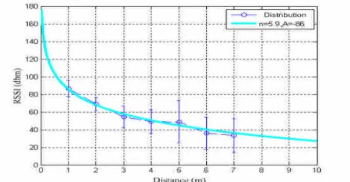
Figure 1 is the experimental result in an indoor corridor environment using ZigBee:

Figure 1. RSSI measurements and model

The measurement statistics distributions, include averages and standard deviations of RSSI at different distances, are shown in the figure in deep blue color. A model with parameters n=5.9 and A=-86 is determined to be the best fit for the case. From figure 1 it can be seen that the measurement noise increase with distance. The uncertainties caused by the noises make the accurate identification of n and A difficult. For example, fix A and varying n from 3.9 to 8.9 or fix n and varying A from -76 to -96 all produce RSSI model curves that fit within the measurement distributions. Tests in other environments (not shown) have different model parameters.

RSSI BASED POSITION DETERMINATION

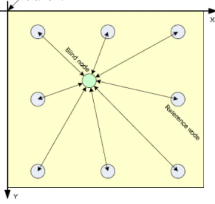
Figure 2 shows a simplified system for two-dimensional location detection based on RSSI [9].

Figure 2. RSSI Location System [9]

In the figure, “reference nodes”are static nodes placed at known positions while “blind node”isanodethat receive RF signals from all reference nodes and read out the respective RSSI values . Distances from the blind node to various reference nodes are derived from RSSI measurements and these can be used to calculate the position of the blind node. Consider m reference nodes with known positions (x₁, y₁), (x₂, y₂), …, (x_m, y_m), and a blind node with unknown position (x, y). With m RSSI measurements, at any time instance k one can write

 

 





) (

) ( )

( ) ( log 10 ) (

) ( )

( ) ( log 10 ) (

2 2

2 2 2 2 2 2 2

2

1 1 2 1 2 1 1

1

k v A y y x x n k RSSI

k v A y y x x n k RSSI

k v A y y x x n k RSSI

m m m m

m      































(2)

where RSSI₁(k), RSSI₂(k), …, RSSI_m(k) are the RSSI measurements at blind nodes from each reference nodes, and v1(k), v2(k), …, vm(k) are the corresponding measurement noises and are assume zero mean, white, and Gaussian.

To study various positioning methods, a simulation environment is setup first and the blind node is assumed to be travelling along a square path with constant velocity 10cm/sec (figure 3).

Figure 3. Simulation path for the blind node The square path has 4 equal side length of 250 cm and the blind node travel in clockwise direction, starting from (0, 5). Four reference nodes are placed at coordinates (0, 0), (200, 0), (200,400) and (0, 400). The reference nodes are assumed to have the same RSSI model with parameters n=8 and A=-80 respectively.

In the simulation, measurement noises v₁, v₂, v₃and v₄are assumed to have standard deviationv= 8. From figure 1 one can see that such noise level matches real situation.

Ideal and measured RSSI at different locations are shown in figure 4, where green lines indicated the ideal RSSI values at different positions at different time, while the blue lines are the measured RSSI values with noises used in subsequent simulation studies.

Figure 4. Ideal and measured RSSI at different locations Several different methods for calculating the blind node positions using the RSSI measurements are presented next.

 RLS solution

By usingt the RSSI model, distances between the blind node and refernce nodes can be calculated from the measured RSSI values:

4 , 1 , 10

)

ˆ( ¹⁰

) (

 



 

j k

d ^j

j j

n k RSSI A

j (3)

The blind node positions can be solved from the following equations:

) ( ) ( ) ( ) ˆ(

) ( ) ( ) ( ) ˆ(

) ( ) ( ) ( ) ˆ(

) ( ) ( ) ( ) ˆ(

4 2 4 2

4 4

3 2 3 2

3 3

2 2 2 2

2 2

1 2 1 2

1 1

k v y y x x k d

k v y y x x k d

k v y y x x k d

k v y y x x k d











































(4)

where v^’_j(k) are the distance errors resulting from RSSI measurement errors v_j(k).

Solution for blind node positions (x, y) that minimize the square sum of the distance errors can be derived by using RLS (Recursive Least Square) estimation. Figure 5 shows the RLS solutions of the blind nodes.

Figure 5. RLS position estimate result

The accuracy of the blind position estimates will depend on the RSSI measurement error covariancev. In reality, the RLS position estimates of the Zigbee system have accuracy in the order of a few meters and may not be accurate enough for some applications. To improve the position estimate accuracy, knowledge of the blind node motions should be utilized and optimal state estimation theories such as Kalman Filter [12] can be used.

 Kalman filtering with motion models

Instead of allowing the blind node motion to be completely random, motion model which relates the current blind node position with previous ones can be used to improve the estimation. The simplest motion model is to assume the blind node position at time instance k+1 are the position at last time instance k plus some random motion. This model is called P-model and was used to model the famous Brownian motions. Using the blind node position (x, y) as states, the P-model can be written as the following state equation:

) ( ) ( ) 1 (

) ( ) ( ) 1 (

k w k y k y

k w k x k x

y x











 (5)

with the RSSI measurement equations:

 

 

 





) (

) ( )

) ( ( ) ) ( ( log 10 ) (

) ( )

) ( ( ) ) ( ( log 10 ) (

) ( )

) ( ( ) ) ( ( log 10 ) (

4 4 2 4 2

4 4

4

3 3 2 3 2

3 3

3

2 2 2 2 2

2 2

2

1 1 2 1 2

1 1

1

k v A y k y x k x n k RSSI

k v A y k y x k x n k RSSI

k v A y k y x k x n k RSSI

k v A y k y x k x n k RSSI























































 . (6)

In equation (5), w_x and w_y are the relative displacements of the blind node and are assumed to be random, since one does not have advanced knowledge of the motions.

To accommodate the actual displacement range of 10cm in the simulation study, w_xand w_yare assumes to be zero mean, white, Gaussian with covariance of 100 cm². Since the measurement equations are nonlinear, EKF (Extended Kalman Filtering) [12] method can be used to estimate the blind node positions. Figure 6 show the blind node position estimate using EKF with P-model. Comparing figure 5 with figure 6, it is clear that the blind node position estimation is greatly improved by using EKF.

Figure 6. Position estimate using EKF with P-model Instead of describing the blind node motion using the P- model, a higher order motion model called PV-model that describe a constant velocity motion can be used and it matches more closely to the actual blind node motions in the simulation study. The state equation using the PV- model can be written as:

) ( ) ( ) 1 (

) ( ) ( ) 1 (

) ( ) ( ) 1 (

) ( ) ( ) 1 (

k w k y k y

k w k x k x

k y k y k y

k x k x k x

y x









































(7)

where the new statesx, y are the relative displacements of the blind node and they are assumed to be different from the relative displacements at previous time instance by zero mean, white Gaussian noises w_x, w_y. In this study w_x, w_y are both assumed to have covariance of 1 cm². Together with the measurement equation (6), EKF can be used to estimate the blind node positions. Figure 7 show the position estimate using EKF with PV-model.

As PV-model has a smaller process covariance matrix comparing with P-model, the position estimates take more motion dynamic model information into account. Since the PV-model does describe the actual blind node motion more accurately, the estimation result is more accurate.

Figure 7. Position estimate using EKF with PV-model DEAD-RECKONING AIDED RSSI POSITIONING When dead-reckoning sensors are available, relative displacements can be measured directly and treated as inputs instead of being considered as a state for estimation.

The blind node motion can be desribed by the state equation below:

) ( ) ( ) ( ) 1 (

) ( ) ( ) ( ) 1 (

k w k y k y k

y

k w k x k x k x

y x



















 (8)

or

) ( ) ( ) ( ) 1

(k xk u k w k

x     ^.

Where x=(x, y)^T is the state vector, u=(x, y)^T is the input vector using dead-reckoning measurements, and w=( w_x, w_y)^Tis the process noise vector which is resulted from dead-reckoning measurement errors and is assumes to be zero mean, white and Gaussian. The process covariance matrix Q=E[w^Tw] is assumed to be diag(25, 25) in the simulation study.

With the more accurate motion model and the exact knowledge of relative displacement as inputs, the accuracy of the blind node positions estimates can be further improved, as shown in figure 8. The RMS of the positioning errors is calculated as 33 cm, which is an order of magnitude better than the RLS positioning accuracy.

Figure 8. Position estimate using EKF with DR inputs DR-AIDED RSSI POSITIONING IN DYNAMIC ENVIRONMENTS

In reality, parameters for RSSI model can be varying in different environments. When positioning in dynamic indoor environments, one can move from one environment to another with different RSSI model. It is impossible to expect a set of RSSI model parameter to work in all environments and large positioning errors can resulted from parameter mismatches. In the simulation below, RSSI model parameter n and A for all the reference nodes under the environment are assumed to be 6 and -80. Two studies are conducted. In the first study, the parameter A is set to -90 initially to match a case that the reference node signal strength is varying due to different transmitter power setting change or antenna gain changes resulted from different orientation. In the second study, both parameters n and A are set to 5 and -90 initially to simulate a change of environment.

 Dynamic Environment with parameter A change Figure 9 show that with incorrect RSSI model parameter A, even with the aiding of dead-reckoning information,

the position estimation will exhibit large errors. In figure 9, the RMS of position errors is 158 cm, almost 5 times of figure 8.

Figure 9. Position estimate with incorrect parameter A To deal with the changing parameter in different environments, the system formulation can be modified to include the RSSI model parameter A as states for estimation. The new state equation can be written as:























































































































) (

) (

) (

) (

) (

) (

0 0 0 0 ) (

) (

) (

) (

) (

) (

) (

) (

) 1 (

) 1 (

) 1 (

) 1 (

) 1 (

) 1 (

4 3 2 1

4 3 2 1

4 3 2 1

k w

k w

k w

k w

k w

k w k y

k x

k A

k A

k A

k A

k y

k x

k A

k A

k A

k A

k y

k x

A A A A y x

(9)

with measurement equation:

 

 

 





) (

) ( ) ( ) ) ( ( ) ) ( ( log 10 ) (

) ( ) ( ) ) ( ( ) ) ( ( log 10 ) (

) ( ) ( ) ) ( ( ) ) ( ( log 10 ) (

4 4 2 4 2

4 4

4

3 3 2 3 2

3 2

3

2 2 2 2 2

2 2

2

1 1 2 1 2

1 1

1

k v k A y k y x k x n k RSSI

k v k A y k y x k x n k RSSI

k v k A y k y x k x n k RSSI

k v k A y k y x k x n k RSSI























































 . (10)

In equations (9) and (10), the RSSI parameter A are denoted as A_j(k), j=1,..,4, and are allowed to change with time. EKF as well as Particle Filter (PF) [13] are used to estimate the positions and RSSI model parameters simultaneously. Figure 10 shows the blind node position estimate. The final position estimates for EKF and PF both converge to a level similar to figure 8.

Figure 10. Position estimate with parameter A changes

 Dynamic Environment with both parameters change

Figure 11 show the positioning result with both RSSI model parameters n and A incorrect. Comparing with figure 9 the positioning errors of figure 11 are even worse.

Figure 11. Position estimate with incorrect A and n To deal with the changing parameters in different environments, the system formulation is modified to include all RSSI model parameters as states for estimation.

The new state equation is:















































































































































































) (

) (

) (

) (

) (

) (

) (

) (

) (

) (

0 0 0 0 0 0 0 0 ) (

) (

) (

) (

) (

) (

) (

) (

) (

) (

) (

) (

) 1 (

) 1 (

) 1 (

) 1 (

) 1 (

) 1 (

) 1 (

) 1 (

) 1 (

) 1 (

4 3 2 1 4 3 2 1

4 3 2 1 4 3 2 1

4 3 2 1 4 3 2 1

k w

k w

k w

k w

k w

k w

k w

k w

k w

k w k y

k x

k A

k A

k A

k A

k n

k n

k n

k n

k y

k x

k A

k A

k A

k A

k n

k n

k n

k n

k y

k x

A A A A n n n n y x

(11)

with measurement equation:

 

 

 





) (

) ( ) ( ) ) ( ( ) ) ( ( log ) ( 10 ) (

) ( ) ( ) ) ( ( ) ) ( ( log ) ( 10 ) (

) ( ) ( ) ) ( ( ) ) ( ( log ) ( 10 ) (

4 4 2 4 2

4 4

4

3 3 2 3 2

3 2

3

2 2 2 2 2

2 2

2

1 1 2 1 2

1 1

1

k v k A y k y x k x k n k RSSI

k v k A y k y x k x k n k RSSI

k v k A y k y x k x k n k RSSI

k v k A y k y x k x k n k RSSI























































 . (12)

Again, EKF and PF are used to estimate the positions and RSSI model parameters simultaneously. Figure 12 shows the positioning result. The result is comparable to figure 10 and the final position estimates converge to similar level as figure 8.

Figure 12. Position estimate with parameters n, A changes

EXPERIMENTS

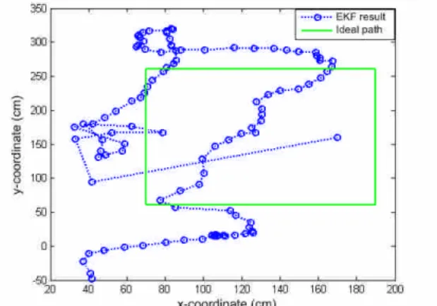
To further verify the result of dead-reckoning aided RSSI- based positioning algorithm under dynamic environments, experiments were conducted in NTUST laboratory.

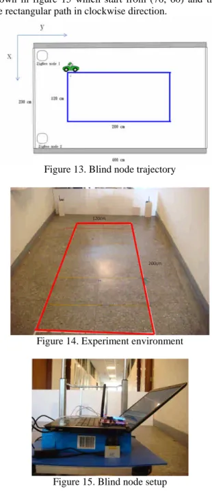
Figures 13 and 14 show the path of the blind node in the experiment and the testing environment. Due to hardware limitations, only 2 Zigbee reference nodes are used in the experiments and their locations are (0, 0) and (200, 0) respectively. The blind node is located on a cart (as shown in figure 15 which start from (70, 60) and travel the rectangular path in clockwise direction.

Figure 13. Blind node trajectory

Figure 14. Experiment environment

Figure 15. Blind node setup

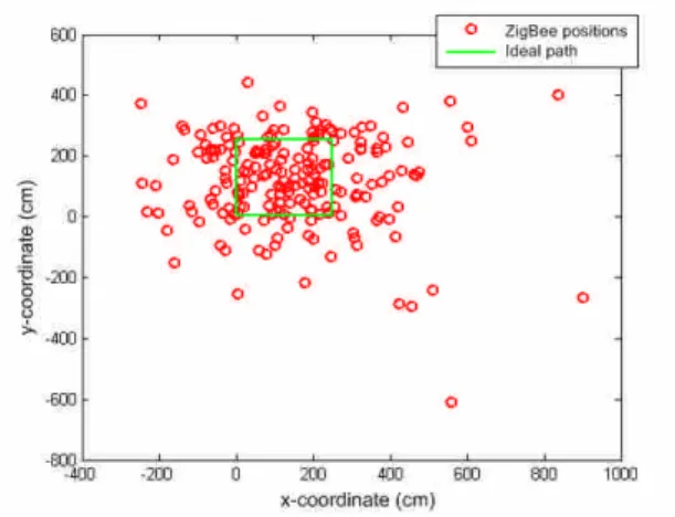
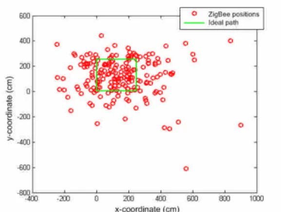
The RSSI model parameters in this environment are first initialized to be n=5.9 and A=-86 for both reference nodes.

They are allowed to change during the experiments by the algorithm. Figure 16 shows the blind node position estimates using the RLS method. This result has error level comparable to figure 5, in the order of a few meters.

Figure 16. RLS position estimate result

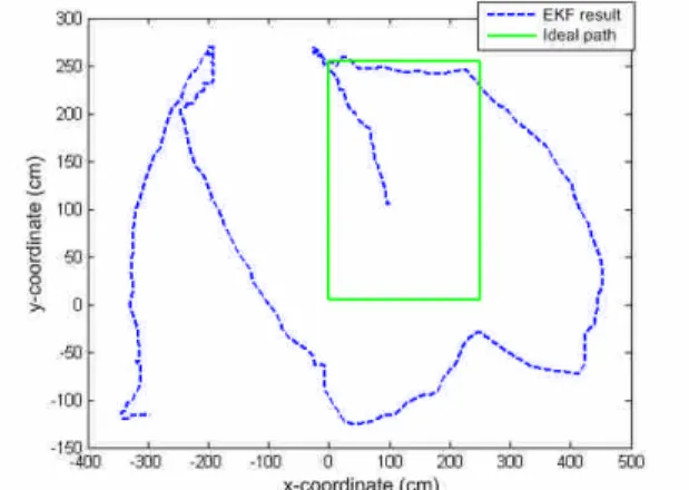
Figures 17 show the position estimate results using EKF with PV models. Due to poor model parameter selection, the estimates have errors for a few meters although the estimated path does resemble the actual path thanks to more trusts in motion model by using the PV-model.

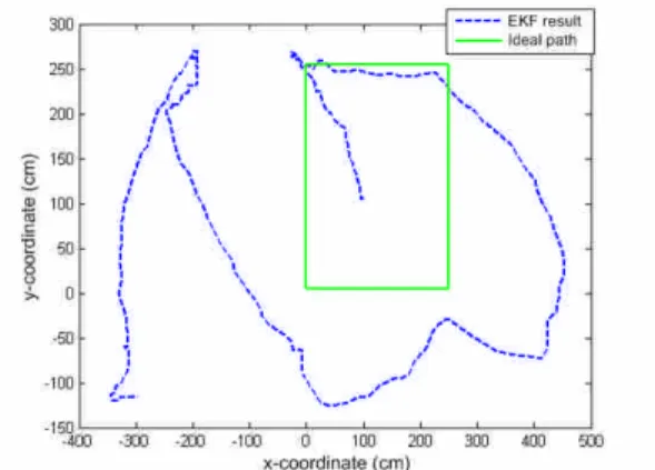
Figure 17. Position estimate using EKF with PV-model Using a laser ranger [14] to scan the surrounding walls and use the ICP (Iterative Closest Point) algorithm [15] to calculate the corresponding relative displacements of the blind mode, dead-reckoning aided RSSI positioning algorithm as in equation (8) is used to calculate blind node positions and the result is shown in figure 18 below.

Figure 18. Position estimate using EKF with DR inputs Although figure 18 represent a good improvement of positioning accuracy comparing with figure 16, the

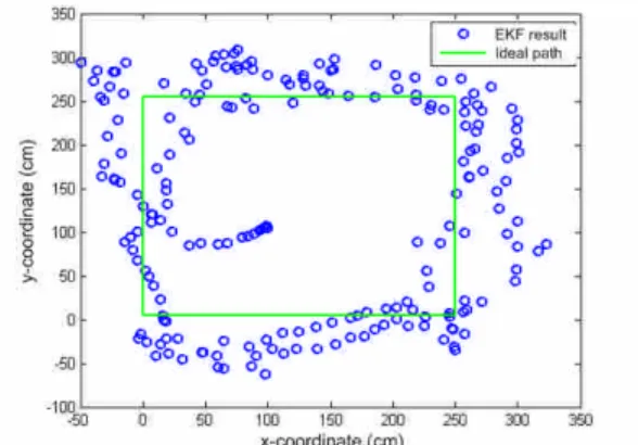
uncertainties of the RSSI model parameters have great impact on the final position estimate accuracy. Therefore the algorithm with RSSI model parameter estimation, as in equations (11) and (12), should be used. Figure 19 shows the positioning result by including parameter estimation, using PF. The position estimates have good accuracy with most errors under 0.5 meters.

Figure 19. Position estimate using DR-aided PF with parameters estimation

CONCLUSION

A RSSI positioning method that estimates both the unknown user locations as well as the changing RSSI model parameters in dynamic indoor environments was proposed. The algorithm use the relative displacements measured by dead-reckoning systems as inputs and nonlinear state estimators such as EKF and Particle filter can be used to estimate the unknown states. Since the knowledge of RSSI model parameter is not required, the method is more suitable to practical situation that the user can travel in different indoor environments. Advanced calibration of RSSI model parameters for the navigation environments is not necessary. Through both simulations and experimental studies, it is demonstrated that the method can increase the positioning accuracy for a DR- aided Zigbee system from a few meters to decimeter levels.

ACKNOWLEDGEMENT

This research is sponsored by Taiwan National Science Council under grant NSC99-2221-E-011-125.

REFERENCE

[1] I. Guvenc, C. Abdallah, R. Jordan, and O. Dedeoglu, Enhancements to RSS Based Indoor Tracking Systems Using Kalman Filters, Proc. of the Global Signal Processing Conf. (GSPx), pp. 91-102, 2003.

[2] A.H. Sayed,A. Tarighat,and N. Khajehnouri, Network-based wireless location, IEEE Signal Processing Magazine, pp 24-40, July 2005.

[3] M. Sugano, T. Kawazoe, Y. Ohta, and M. Murata, Indoor Localization System Using RSSI Measurement of Wireless Sensor Network Based on ZigBee Standard, The IASTED International

Conference on Wireless Sensor Networks (WSN 2006), Banff (Canada), July2006.

[4] S. Tennina, M. Di Renzo, F. Graziosi, and F.

Santucci, Locating Zigbee^® nodes using the TI^®s cc2431 location engine: a testbed platform and new solutions for positioning estimation of WSNs in dynamic indoor environments, Proceedings of the first ACM international workshop on Mobile entity localization and tracking in GPS-less environments, San Francisco, pp. 37~42, 2008.

[5] E. Lau, B. Lee, S. Lee, and W. Chung, Enhanced RSSI-Based High Accuracy Real-Time User Location Tracking System for Indoor and Outdoor Environments, International Journal on Smart Sensing and Intelligent Systems, Vol. 1, No. 2, June 2008.

[6] P. Barsocchi, S. Lenzi, and S. Chessa Self- Calibrating RSSI-based Indoor Localization with IEEE 802.15.4, Technical Report ISTI-2008-TR-01, Istituto di Scienza e Tecnologie dell'Informazione del CNR, Pisa, Italy, January 2008.

[7] L. Fang, et al., Design of a Wireless Assisted Pedestrian Dead Reckoning System - The NavMote Experience, IEEE Trans. Instrumentation and Measurement, Vol. 54, pp. 2342-2358, December 2005.

[8] A. Davison, Real-time simultaneous localisation and mapping with a single camera, Proc.

International Conference on Computer Vision, Nice, October 2003.

[9] K. Aamodt, CC2431 Location Engine. Application Note AN042, Texas Instruments.

[10] CC2430 A True System on Chip solution for 2.4 GHz IEEE 802.15.4/Zigbee datasheet, Chipcon 2007.

[11] D. Lymberopoulos, Q. Lindsey, and A. Savvides, An Empirical Analysis of Radio Signal Strength Variability in IEEE. 802.15.4 Networks Using Monopole Antennas, The 3rd European Workshop on Wireless Sensor Networks, pp. 326-341, 2006.

[12] G. Welch and G. Bishop, An Introduction to the Kalman Filter, UNC-Chapel Hill, TR 95-041, March 11, 2002.

[13] M. Arulampalam, S. Maskell, N. Gordon, T. Clapp, A Tutorial on Particle Filters for Online Nonlinear/Non-Gaussian Bayesian Tracking, IEEE Transactions on Signal Processing, Vol. 50, No.2, pp 174-189. February 2002.

[14] Range-Finder Type Laser Scanner URG-04LX Specifications, Kokuyo Automatic Co. Ltd., 2005.

[15] Paul J. Besl, and Neil D. McKay, A Method for registeration of 3-D shapes, IEEE Transactions on Pattern Analysis and Machine Intelligence, Vol. 14, No. 2, pp. 239-256,1992.

表 Y04

行政院國家科學委員會補助國內專家學者出席國際學術會議報告

100 年 12 月 7 日 報告人姓名

高維文 服務機構

及職稱 國立台灣科技大學機械系副教授

時間 會議

地點

2010.9.21~2010.9.24

Portland, Oregon, USA

本會核定 補助文號

NSC- 99-2212-E011-125

會議 名稱

(中文)美國導航學會 2010 全球導航衛星系統年會 GNSS-2010 (英文)ION GNSS-2010

發表 論文 題目

(中文)方位推估輔助之室內動態環境 RSSI 定位法

(英文) Dead-reckoning Aided RSSI Based Positioning System for Dynamic Indoor Environments

表 Y04

一、參加會議經過

美國導航學會（Institute of Navigation, ION）成立於 1945 年，為美國專注於導航領域之 專業學會，每年舉辦數次不同主題之學術研討會，ION-GNSS 會議為 ION 每年一度主題為衛 星定位與導航系統的會議，亦為全球在此領域的最重要會議。此會議慣例於每年九月份舉行 並每二年更換會議地點，ION-GNSS 2010 年會於 2010 年 9 月 21 日至 24 日於奧勒岡州波特 蘭市舉行。此次會議除來自美國與加拿大的學術與研究單位外，還有包含歐洲、亞洲等相關 領域人士參加。

除學術會議外，大會並有相關產業儀器設備展覽，許多 GPS 領域的領導廠商過去往往也 選擇在此一盛會發表最新產品與相關技術。近年由於 GPS 商業應用已非常發達，因此較具商 業性的 GPS 相關產品有轉移到 CES，CeBIT 等消費性電子產品展覽的趨勢，但專業的衛星接 收器廠商及國防工業的供應商仍多選擇此一展覽展出產品。

本人於 9 月 21 日晚間經舊金山飛抵 Portland 市，因班機時間因素無法參加 21 日晚間之 開幕式，於 22 日上午開始參加相關之論文研討會。近年由於導航應用環境的變化，導航研究 開始轉往多感測器的整合，ION-GNSS 會議的相關議題已不侷限於衛星定位系統之研究，會 議分項討論議題如下：

September 22, 2010

Morning Afternoon

B1 GNSS Algorithms and Methods 1 A2 GPS IIF: From Inception to Launch Integrated Sensors

C1a Autonomous Vehicles B2 GNSS Simulation and Testing C1b RAIM and/or Multi-Constellation

RAIM

C2 Enhanced and Developing Systems D1 Atmospheric Sciences D2 Remote Sensing with GNSS &

E1 Urban and Indoor Navigation Technology 1

E2a Consumer Applications

E2b Regulatory Service Applications (Road user Charging, etc.)

F1 Pedestrian Navigation F2 LBS Technology and Applications P1 Program Updates: GPS, GLONASS,

Galileo, COMPASS, IRNSS, QZSS

P2 Program Updates: High Integrity Systems

September 23, 2010

Morning Afternoon

A3 Integrating System Capabilities at the GPS Wing (Invited Papers Only)

A4 NATO Military PNT & NAVWAR (Invited Papers Only)

B3 New Product Announcements B4 Software Receivers

C3 Aviation Applications C4 GNSS Space Based Augmentation Systems (SBAS)

D3 Surveying and Geodesy D4a Marine Navigation

D4b Timing & Scientific Applications E3 GPS and GLONASS Modernization and

Other Emerging GNSS (Galileo, QZSS, IRNSS, COMPASS)

E4 Integrity Monitoring for Next Generation Applications

F3 Land Based Applications F4 Urban and Indoor Navigation Technology 2

表 Y04

P3 Deep Indoor Navigation Which Technologies Will Prevail?

P4 50th Anniversary of Kalman Filtering September 24, 2010

Morning Afternoon

A5 Military GPS and Host Applications Integrations for Robust PNT Solutions B5 Precise Point Positioning and Network RTK

B6 Statistical Signal Processing C5 GNSS Ground Based Augmentation

Systems (GBAS)

C6 Next Generation GNSS Integrity for Aviation

D5 Space Applications D6 GNSS Algorithms and Methods 2 E5 Multi-Constellation User Receivers E6 Galileo System Design and Services,

GPS/Galileo Interoperability F5 Portable Navigation Devices F6 Urban and Indoor Navigation

Technology 3 P5 Common Frequencies vs. Frequency

Diversity in Civil Signals — What is the Right Choice?

P6 The Use of GNSS in Emergency Services

藍字部分為我較長程參與場次。

由討論議題分項可看出近年衛星定位系統已由過去專注於美國之 GPS 系統擴展至歐盟的 Galileo 與俄羅斯的 Glonass 系統，導航技術則已由之前專注於衛星定位系統之研究轉移至與 其他感測器整合之技術，在應用領域則由傳統之航海、航空應用擴展到陸地車輛、行人、及 室內應用。由於本人近年研究領域偏向行人定位與室內無衛星狀況下的定位應用，因此亦選 擇相關議題論文發表場次，計參加以下論文發表：

9 月 22 日：

F1-2: “I

n-Situ Step Size Estimation Using a Kinetic Model of Human Gait,”C. Matthews, Y.

Ketema, D. Gebre-Egziabher, M. Schwartz, University of Minnesota - Twin Cities

F1-3: “

Assessment of Indoor Magnetic Field Anomalies using Multiple Magnetometers,”M.H.

Afzal, V. Renaudin, G. Lachapelle, University of Calgary, Canada

F1-4: “

Vision-aided IMU for Pedestrian Navigation,”C. Hide, University of Nottingham, UK;

T. Botterill, M. Andreotti, University of Canterbury, New Zealand

F1-5: “

Non-conventional INS/GNSS Integration for Qualitative Motion Analysis in Caregiving Applications,”P. Molina, I. Colomina, Institute of Geomatics, Spain; M. Troger, B.

Hofmann-Wellenhof, TeleConsult Austria; C. Aguilera, European GNSS Supervisory Authority, Belgium

F1-6: “T

owar ds Ar bi t r ar y Pl ac ement of Mul t i -sensors Assisted Mobile Navigation System,”X.

Zhao, S. Saeedi, University of Calgary, Canada; Z. Syed, C. Goodall, Trusted Positioning Inc., Canada

F1-7: “

Test Results for Indoor Positioning Solution using MEMS Sensor Enabled GPS Receiver,”M. Chowdhary, M. Jain, R. Srivastava, SiRF Technology

F1-8: “

A Novel EMG-based Stride Length Estimation Method for Pedestrian Dead Reckoning,”W. Chen, University of Science and Technology of China, China

E2-1: “

Robust First Fix Performance in Urban Areas,”Y-C. Chien, W.G. Yau, W-H. Ting, Z-H.

表 Y04

You, H-J. Chen, A-B. Chen, Y-W. Ting, C-W. Chen, W-C. Tsai, MediaTek Inc., Taiwan

F2-2: “De

vel opment of a Real Ti me I ndoor Locat i on Bas ed Ser vi ce Tes t Be d,”L-T. Hsu, W-M.

Tsai, S-S. Jan, National Cheng Kung University, Taiwan

F2-3: “Re

s ul t s of IMES Implementation for Seamless Indoor Navigation and Social Infrastructure Platform,”D. Manandhar, H. Torimoto, S. Kawaguchi, GNSS Technologies Inc.,

E2-4: “

GNSS Position Computation without Ep he mer i s “Si ngl e Shot MS Bas ed”,”J. de Salas,

F2-5: “De

mons t r at i on of I nt e r -Vehicle UWB Ranging to Augment DGPS for Improved Relative Positioning,”M.G. Petovello, K. O´Keefe, B. Chan, University of Calgary, Canada

9 月 23 日 Panel Discussion 3：Deep Indoor Navigation –Which Technologies Will Prevail?

此一討論主要在探討在室內定位領域的各項技術與產業發展的狀況，參與的專家與業者 討論的題目包含

1. Deep Indoor Navigation –The End of the Beginning: Dr. Frank van Diggelen, Broadcom Corporation

3. Pseudolite Concepts for Deep Indoor Navigation: Dr. Stewart Cobb, Novariant Corporation 4. MOSAIC: Enabling Technology for Deep Indoor Navigation: Prof. Changdon Kee, Seoul National University, South Korea

5. WiFi Localization: Market, Technology, and Future: Farshid Alizadeh-Shabdiz, Skyhook Wireless, Inc.

6. IMES (Indoor Messaging System) The Solution for Deep Indoor Navigation: Mr. Kiyoshi Yajima, Lighthouse Technology and Consulting Co., Ltd., Japan

9 月 24 日：

主要工作為在 Urban & Indoor Navigation Technology Session 3 發表論文 F6-1: “De

ad-reckoning Aided RSSI Based Positioning System for Dynamic Indoor Environment,”W-W. Kao, National Taiwan University of Science and Technology, Taiwan

9 月 22 日中午在展覽場進行午餐，場內主要攤位為國防廠商如 Boeing，Lockheed Martin，

高端衛星定位儀廠商如 Javad，Trimble，Novatel，Topcon，Spirent 及一些衛星定位相關政府 機構如 Galileo 及 IFEN 等，其他較小攤位則為一些感測器元件，天線，系統整合廠商等。

9 月 24 日午間則參加 ION 舉辦之頒獎午宴，頒發 Kepler Award 及 Parkinson Award，前者 為頒發給對衛星定位技術發展有卓越貢獻之學者，本年度頒發給 Dr. Todd Walter，主要表彰他 在 WAAS 領域的貢獻。後者則頒發給在衛星定位領域研究的優秀畢業研究生，本年度頒給 University of Calgary 的 Dr. Ali Broumandan。由於班機行程，我於頒獎午宴後便離開 Portland 市，於 9 月 26 日清晨經舊金山返抵桃園國際機場。

二、與會心得

由於本人近年研究領域轉向室內與行人定位的應用，因此對行人方位推估法的研究進展 極有興趣，第一天上午參加 F1：Pedestrian Navigation 及下午的 F2：LBS Technology and Applications 分組。在 F1 session 的研究包含不少個人運動模式的分析，並多所著墨於各種不