The Design and Realization of a DSP-based Power Electronic Circuit Real-Time Simulator
Chi-Shan Yu Member, IEEE
Department of Electrical Engineering National Taipei University of Technology
Taipei, Taiwan [email protected]
Bo-Chin You
Department of Electrical Engineering National Taipei University of Technology
Taipei Taiwan.
[email protected]
Jack W. Smith
Department of Electrical Engineering National Taipei University of Technology
Taipei Taiwan.
[email protected]
Abstract -- In order to design a high performance power electronics circuit, a precise simulation environment is essential for the controller design. In this paper, a power electronic circuit real-time simulator was designed and realized on a DSP chip. The dynamic equations of a power electronics circuit were coded on a Texas Instruments (TI) made C6416 fixed point DSP.
Meanwhile, the interrupt interface of the DSP was used to capture the pulse-width modulation (PWM) signal. Thus, the switching waveforms can be computed by a single DSP chip. To output the obtained waveforms in real-time, the SIGNALWARE ORS-114 AD/DA card was interfaced with the DSP chip by the direct memory access (DMA) channel. Thus, the circuit equation computations and the DAC output operations can be achieved in parallel.
Finally, the designed simulator is used to simulate a 50kHz switching power supply and controlled by a TI C2808 DSP controller. The results show that the proposed hardware simulator can achieve better responses than the conventional software simulators. .
Index Terms—real-time simulator, interrupt, pulse-width modulation, direct memory access.
I. I NTRODUCTION
The power electronics simulation techniques can be mainly categorized as the off-line simulation and the on-line simulation. Generally, the widely used EMTP, IsSpice and the MATLAB are the off-line simulators which can only virtually simulate a power electronics circuit by off-line.
Thus, the on-line controllers and the protection circuits cannot be easily verified by them. In contrast to the off-line simulator, the on-line simulator can achieve a real-time simulation which can interface with the on-line controllers and the protection circuits for verifications.
T ABLE 1T HE PERFORMANCE OF REAL - TIME SIMULATORS
MERITS DRAWBACKS
z Easy to change a simulation environment z Safer and faster to
develop a simulation environment
z The computation speed is very important z It is not easy to build
an accurate simulation environment
In the past, most of the real-time simulators were achieved by using the analog circuit-based platform. Due to the fast progressions of digital circuit, the real-time simulators have been gradually transformed to the analog- digital mixed mode simulation and the full-digital simulator.
By using the full-digital simulator, the engineers can achieve a small size and flexible tuning simulation environment. Thus, the real-time simulation has become a famous technique [1-4]
in designing a power electronics circuit. The merits and the drawbacks of a digital real-time simulator are summarized in Table 1.
The main purposes of this paper is to discuss the power electronics real-time simulator. By using a single DSP chip, the PWM and the switching waveforms of a buck dc-dc step down converter can be accurately simulated. The simulation results have been compared with the off-line simulation platforms (MATLAB and the IsSpice) to verify the accuracy and effectiveness of the proposed real-time simulator
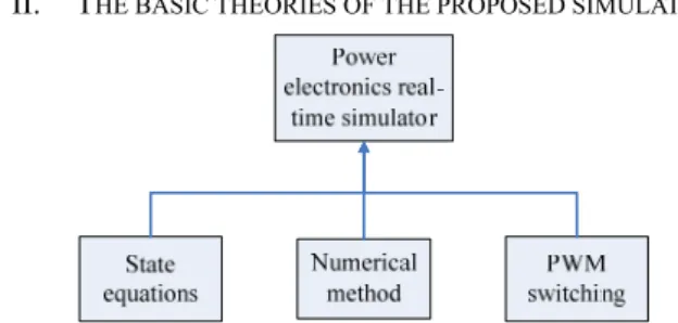
II. T HE BASIC THEORIES OF THE PROPOSED SIMULATOR
Figure 1 Power electronics real-time simulator block diagram
To achieve a power electronics simulator, we need to realize the system state equations, the numerical computations, as well as the PWM computations on a DSP chip. The block diagram shown in Fig. 1 describes these three parts. In this paper, a dc-dc buck converter was utilized to realize the proposed real-time simulator. First, the state equations are described as follows:
iR
ic
vo iL
vC
ic
vo iR
iL
vC
(a) turn-on circuit (b) turn-off circuit Figure 2 The circuit used for developing a real-time simulator
1.Switch turn-on equations
PEDS2009
1239
From the turn-on circuit shown in Fig.2(a), we can have the following equations:
L R L L in
L di i R i r V
dt + + = (1)
R L C L C
i i i i C dv
= − = − dt (2)
1 ( )
L in L L R
di V i r i R
dt = L − − (3)
( ) ( )
C C L
C C
dv v Ri
dt = − C R r + C R r
+ + (4) 2.Switch turn-off equations
From the turn-off circuit shown in Fig.2(b), we can have the following equations:
L
0
R L L
L di i R i r
dt + + = (5)
R L C L C
i i i i C dv
= − = − dt (6)
1 ( )
L L L R
di i r i R
dt = L − − (7)
( ) ( )
C C L
C C
dv v Ri
dt = − C R r + C R r
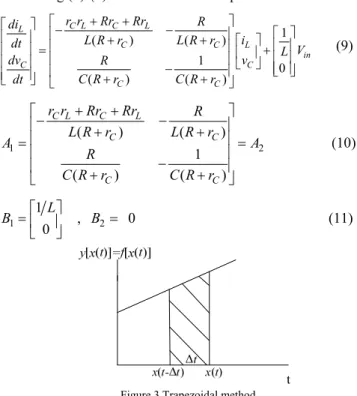
+ + (8) Combining (1)-(8)can achieve a state equation as follows:
( ) ( ) 1
1 0
( ) ( )
C L C L
L
L
C C
in
C C
C C
r r Rr Rr R
di
i
L R r L R r
dt L V
dv R v
C R r C R r
dt
+ +
⎡ ⎤
⎡ ⎤ ⎢ − − ⎥ ⎡ ⎤
⎢ ⎥ ⎢ + + ⎥ ⎡ ⎤ ⎢ ⎥
⎢ ⎥ = ⎢ ⎥ ⎢ ⎥ ⎢ ⎥ +
⎢ ⎥ ⎢ − ⎥ ⎣ ⎦ ⎢ ⎥ ⎣ ⎦
⎢ ⎥ + +
⎣ ⎦ ⎣ ⎦
(9)
1 2
( ) ( )
1
( ) ( )
C L C L
C C
C C
r r Rr Rr R
L R r L R r
A A
R
C R r C R r
+ +
⎡ − − ⎤
⎢ + + ⎥
⎢ ⎥
= =
⎢ ⎥
⎢ + − + ⎥
⎣ ⎦
(10)
1
1 0 B ⎡ L ⎤
= ⎢ ⎥
⎣ ⎦ , B
2= 0 (11)
Figure 3 Trapezoidal method
Then, we used the numerical method to obtain the accurate state values. Using the trapezoidal method shown in Fig. 3, the new state ( ) x t can be obtained as follows:
( ) ( ) { [ ( )] [ ( )]}
2
x t = x t − Δ + t Δ t f x t + f x t − Δ t (12)
Substituting (8)-(11) into (12), we can obtain the voltage and current values step-by-step.
To identify the switching states, this paper used two external interrupts supported by a DSP chip to capture the switching states. As soon as the DSP received a PWM transition signal, the first interrupt subroutine (ISR) was utilized to identify the PWM turn-on time. When the PWM turn-on time has been identified, the second ISR was used to obtain the turn-off time and the duty cycle.
Figure 4 shows the proposed simulation procedures. Since the selected DSP chip has a very fast speed, this paper used the fixed-step computation method to obtain the system states.
At the beginning of each switching period, the state was obtained by using the turn-on equations. When the switching off time was captured by ISR, the numerical equations were changed to the turn-off equations. In the case shown in Fig. 4, the switch turn-off time was captured at t1 and the turn-off equations were used until the next switching period begins.
Switching turn off time
t
Numerical Step
( ) x t x(1)
(2) x
(3) x
Δ t
t1 t2 t3(0) x
Δ t
t1 t2 t3 00 t
Figure 4 Fixed-point simulation
IV. R EALIZATION AND V ERIFICATION
Figure 5 The configuration of the proposed real-time simulator
This paper used a C6416 DSK [5] to realize the proposed real-time simulator and used a C2808 DSK to design a digital controller for closed-loop simulations. The configuration of the proposed real-time simulator is shown in Fig. 5. The above part in Fig.5 denotes the real-time simulator, in which the system state equations are computed in the C6416 DSP chip by fixed-point computations, the analog signals are output by using a daughter DAC board, and the PWM signals are captured by an ISR interface. The below part in Fig.5
PEDS2009
1240
denotes the digital controller which receives the analog signal output from the DAC board and generates appropriate PWM signals to the real-time simulator. To accelerate the simulation speed, the SIGNALWARE ORS-114 board was used in this paper. The main benefit of this board is that the direct memory access (DMA) channel can be designed to communicate between the DAC board and the DSK board.
By using the enhanced DMA channel supported by DSP chip, the obtained voltage and current states can be automatically moved from the DSP memory to the DAC memory. Thus, the simulation speed will not be degraded by the DAC output computations.
Case 1: Open-loop test
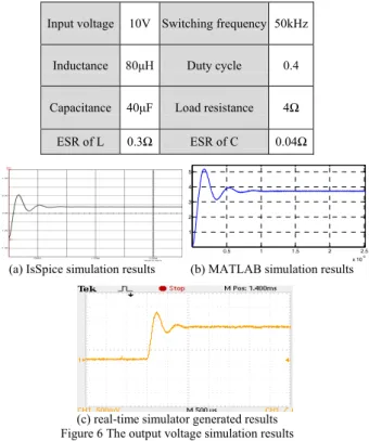
At first, the proposed simulator was simulated on an open- loop condition to evaluate the accuracies of the starting voltage and current waveforms. The fixed point C language was used to program the simulation program of a 50kHz buck dc-dc power supply. Detail parameters of the simulated circuit are listed in Table 1. For comparisons, the simulation results obtained by IsSpice and MATLAB are also performed.
Since the magnitudes of output analog signals are limited by the output capabilities of the DAC daughter card. The voltage signals generated by the real-time simulator are assumed having been reduced by 0.33 time and the current signals are assumed having been reduced by 0.5 time.
T
ABLE1 T
HE PARAMETERS OF A BUCK CONVERTER FOR CASE1
SIMULATIONSInput voltage 10V Switching frequency 50kHz
Inductance 80μH Duty cycle 0.4
Capacitance 40μF Load resistance 4Ω
ESR of L 0.3Ω ESR of C 0.04Ω
0.5 1 1.5 2 2.5
x 10-3 1
2 3 4 5
(a) IsSpice simulation results (b) MATLAB simulation results
(c) real-time simulator generated results Figure 6 The output voltage simulation results
The simulation results of the starting waveform are shown in Fig. 6 and Fig. 7. Fig.6 shows the starting voltage waveforms. Comparing the results of Fig.6(a), Fig.6(b) and Fig.6(c), it can note that the voltage waveform generated by
the real-time simulator is almost the same as those generated by IsSpice and MATLAB. Fig.7 shows the simulation results of the starting current waveforms. It can note that the real- time simulator can also generated accurate current waveforms.
0 2 4 6 8 10 12 14 16
x 10-4 0
0.5 1 1.5 2 2.5
(a) IsSpice simulation results (b) MATLAB simulation results
(c) real-time simulator generated results Figure 7 The inductor current simulation results
Figure 8 (a), (b), and (c) represent the inductor current waveforms generated by the IsSpice, MATLAB, and the proposed real-time simulator, respectively. For comparison, the PWM signal is also shown in Fig.8(c). It can be noted that the current waveform generated by the proposed real- time simulator can accurately respond to the PWM signal. To evaluate the performances of the proposed simulator, all the simulation results are compared in Table 2. It can be noted that the waveforms generated by proposed real-time simulator are almost the same as those generated by the off- line simulators.
5.42 5.44 5.46 5.48 5.5 5.52 5.54
x 10-3 0.2
0.4 0.6 0.8 1 1.2 1.4 1.6
(a) IsSpice simulation results (b) MATLAB simulation results
(c) real-time simulator generated results
Figure 8 The inductor current simulation waveform and PWM signal T
ABLE2 C
OMPARISONS OF THE SIMULATION RESULTSSimulator Settling
time
Steady- state voltage
Steady- state current
Voltage
ripple Current ripple
MATLAB 1.2ms 3.72V 0.9A 36mV 0.6A
IsSpice 1.2ms 3.72V 0.9A 36mV 0.6A
The proposed
simulator 1.2ms 3.7V 0.85A 35.15mV 0.58A
PEDS2009
1241
Case 2: Closed-loop test
In this case, a 4Ω load change was used to test the performance of the proposed simulator under a closed-loop condition. To achieve this, a digital controller was implemented on the C2808 DSP chip by a simple voltage mode control. The designed controller transfer function is as follows:
2 5
1.048 1.009
( ) 3.458 10
c
G z z
z z
−= −
− + × (12)
By using the designed controller, the output voltage of the test circuit was set as 5V. The parameters of the test circuit are listed in Table 3.
T
ABLE3 T
HE PARAMETERS OF A BUCK CONVERTER FOR CASE2
SIMULATIONSInput voltage 10V Switching frequency 50kHz
Inductance 90μH Output voltage 5V
Capacitance 100μF Load resistance 4Ω ESR of L 0.3Ω ESR of C 0.05Ω
Since the IsSpice cannot be used to simulate a circuit under a digital control environment, the remaining simulations are only performed by MATLAB and the proposed real-time simulator. For comparison, a fixed 0.5 duty PWM signal was performed to evaluate the waveform under a open-loop condition and the simulation results are shown in Fig.9. It can be noted that the waveforms generated by the proposed real-time simulator and the MATLAB are almost the same. Then, the C2808 DSP was used, and the closed loop simulation waveforms are shown in Fig.10. It can be noted that the proposed real-time simulator can achieve almost the same waveforms generated by the off-line MATLAB simulator.
0.0245 0.025 0.0255 0.026 0.0265
4 4.2 4.4 4.6 4.8
(a) MATLAB simulation results
(b) The results generated by the proposed real-time simulator Figure 9 The generated voltage waveform with a fixed duty 0.5
0.072 0.073 0.074 0.075 0.076 0.077 0.078 0.079
4 4.5 5 5.5 6