EEG-based Measures of Auditory Saliency in a Complex Context

(1)

EEG-based Measures of Auditory Saliency in a Complex Context

Xun-Yi Huang

Dept. of Computer Science National Chiao Tung

University, Taiwan [email protected]

Fu-Yin Cherng

Jung-Tai King

Brain Research Center National Chiao Tung

Wen-Chieh Lin

ABSTRACT

Auditory saliency is an important mechanism that helps humans ex- tract relevant information from environments. Audio notifications of mobile devices with high saliency can increase users’ receptivity, yet overly high saliency could cause annoyance. Accurately measuring auditory saliency of a notification is critical for evaluating its usability. Previous studies adopted behavioral methods. How- ever, their results may not accurately reflect auditory saliency as humans’ perception of auditory saliency often involves complicated cognitive processes. Thus, we propose an electroencephalography (EEG)-based approach that can complement behavioral studies to provide a more nuanced analysis of auditory saliency. We evaluated our method by conducting an EEG experiment that measured the mismatch negativity and P3a of the sounds in realistic scenarios.

We also conducted a behavioral experiment to link the EEG-based method with the behavioral method. The results suggested that EEG can provide detailed information about how human perceive auditory saliency and complement the behavioral measures.

CCS CONCEPTS

• Human-centered computing → Empirical studies in HCI.

KEYWORDS

Auditory Saliency; Notification; Brain-computer Interface ACM Reference Format:

Xun-Yi Huang, Fu-Yin Cherng, Jung-Tai King, and Wen-Chieh Lin. 2019.

EEG-based Measures of Auditory Saliency in a Complex Context. In 21st International Conference on Human-Computer Interaction with Mobile Devices and Services (MobileHCI ’19), October 1–4, 2019, Taipei, Taiwan. ACM, New York, NY, USA, 11 pages. https://doi.org/10.1145/3338286.3340139

1 INTRODUCTION

The saliency of a sound is defined as its prominence relative to other sounds [41]. Due to humans’ limited brain resources, auditory saliency has evolved as an important mechanism used for filtering irrelevant information from complex and potentially overwhelming auditory environments of the sort one encounters in day-to-day life [8].

Permission to make digital or hard copies of all or part of this work for personal or classroom use is granted without fee provided that copies are not made or distributed for profit or commercial advantage and that copies bear this notice and the full citation on the first page. Copyrights for components of this work owned by others than the author(s) must be honored. Abstracting with credit is permitted. To copy otherwise, or republish, to post on servers or to redistribute to lists, requires prior specific permission and/or a fee. Request permissions from [email protected].

MobileHCI ’19, October 1–4, 2019, Taipei, Taiwan

ACM ISBN 978-1-4503-6825-4/19/10. . . $15.00 https://doi.org/10.1145/3338286.3340139

Auditory saliency plays a critical role in a number of techno- logical applications. Particularly, the auditory saliency of an audio notification can heavily influence its usability. In the field of computer-mediated communication (CMC), audio notifications are one of the essential and useful ways to make users aware of incoming information [29]. A well-designed notification needs to alert users and attract their attention appropriately and timely. Hence, users’ receptivity to an audio notification is crucial for its usability [4, 16]. Prior studies have investigated various factors to users’

receptivity to notifications, including users’ engagement, notification content, and locations [2, 28, 29]. Among all the factors, we consider that whether an audio notification is salient enough as compared to its surrounding sound is a direct and primary indi- cator of whether users receive the notification or not. Moreover, optimizing the auditory saliency of a notification under ambient noise enables users to be notified seemly so that they have well receptivity to the notification. Hence, the quality and accuracy of our ability to measure auditory saliency profoundly influence the evaluation and applications of mobile notifications and other similar applications.

Auditory saliency can be identified from bottom-up processing and top-down processing. The focus of bottom-up saliency is on sounds’ physical attributes (e.g., pitch and intensity) that make them salient, attracting the listener’s attention and shifting it to a new focus. The top-down perspective, on the other hand, considers sounds’ saliency in relation to their meaning, which is related to higher-level processes as well as individuals’ prior knowledge and experiences. Notably, auditory saliency usually involves an interaction between bottom-up and top-down cues [11]. However, prior researches have rarely addressed how these two types of saliency interact [9].

Previous studies on auditory saliency tended to measure or analyze it through behavioral experiments. In such experiments, the participants are usually asked to pay attention to measured sounds, which is different from the daily life scenario. Hence, we are unable to accurately or realistically assess the influence of their auditory saliency. To avoid the bias inherent in listening out for a sound in advance, auditory saliency should be measured passively, i.e., under conditions where the participants are not told to expect to hear a sound. Kaya and Elhilali also indicated that the behavioral-testing protocols suffer from conscious decision-making and might not reflect purely bottom-up processing [22]. Therefore, in this work, we have sought to resolve these problems by developing an Electroen- cephalography (EEG)-based approach for passively/unconsciously measuring auditory saliency.

(2)

MobileHCI ’19, October 1–4, 2019, Taipei, Taiwan Xun-Yi Huang, Fu-Yin Cherng, Jung-Tai King, and Wen-Chieh Lin

We applied EEG analysis to measure human auditory saliency in terms of perception and attention orientation in a complex sound- scape. We utilized two types of neural responses, mismatch negativity (MMN) and P3a, which can reflect the perceptual characteristics of a sound and a person’s cognitive state after s/he heard a novel sound [31, 35]. In the first experiment, we demonstrated that by observing MMN and P3a responses, our EEG-based method accurately reflected the differing levels of auditory saliency of different stimuli, and also shed light on the participants’ perceptual processing of auditory saliency. To test whether the results of our EEG-based method can complement existing behavioral and self- report methods of saliency measurement, we conducted a second experiment, focusing on the ranking of the auditory stimuli, and analyzed whether the results from EEG-based and conventional methods could jointly reveal a more complete picture of cognitive processing of auditory saliency that could be applied to technologi- cal applications.

2 RELATED WORKS

Most studies of saliency have focused on its visual form, and the development of our understanding of visual saliency is relatively mature. Both stimulating (“bottom-up”) and cognitive (“top-down”) factors influence an observer’s attention [17]. The concept of auditory saliency is similar to that of visual saliency. Prior studies have indicated that the former also possesses “bottom-up” and “top- down” properties [8, 22]. However, some research has also pointed out that there are still many unexplored issues related to auditory saliency: notably, how to precisely define this construct and which stimulating features influence the saliency of a sound [6]. Moreover, how to measure the saliency of a sound has not been adequately addressed.

A common approach for measuring auditory saliency and evaluating auditory-saliency model is human rating [23], in which a saliency ranking order is obtained by asking participants to perform multiple pairwise comparisons of all the sounds in an auditory scene.

Human detection experiment measures auditory saliency based on the participants’ ability to detect particular sounds in an auditory scene containing multiple sounds [23]. The latter method assumes that the more salient the sounds are in a complex auditory scene, the more naturally they can grab our attention and, hence, the more easily they can be detected [5]. However, neither human rating nor human detection necessarily targets bottom-up saliency, because the effects of attention are not conclusively removed from either approach [18]: i.e., participants are requested to focus on detecting incoming sound stimuli, which does not closely simulate most real- world situations. Kaya and Elhilali [22] also mentioned that there is little agreement about whether the result of human rating or detection is task-directed or purely based on saliency. For this reason, Duangudom et al. [9] proposed a dual-test experiment aimed at conclusively isolating bottom-up auditory saliency. However, their experiment did not completely rule out the effects of attention, as the participants still needed to identify the measured sounds.

The sounds evaluated in previous auditory-saliency studies have also tended to be simplistic. Kayser et al. [23] dealt with monaural sounds, and isolated each measured sound from background noise in their experiments. However, sounds seldom occur alone; it is rare

to hear only a single sound in most situations. Inspired by Kayser et al.’s study, Tordini et al. [41] presented sounds in pairs under a background noise and asked participants to identify those sounds in a binaural scenario. Tordini et al. defined a sound’s saliency as its perceptibility relative to a background or the other sounds in a scene.

Kaya and Elhilali [21] proposed a new framework for auditory saliency based on the processes of the auditory pathway. Based on the framework, they designed and conducted a series of full- factorial experiments with manipulating the sound features. Ac- cording to factorial conditions, they formed the foreground sound (deviant) by enlarging the feature difference of one sound clip in the background scene. They then asked participants to report whether they heard a salient event during the experiment. They reported the interactions of these features and mentioned the potentials of using MMN as a measurement of change detection across sensory modalities.

3 BACKGROUND OF BRAIN-SENSING TECHNIQUES

In neuroscience, considerable research efforts have been directed toward measuring the brain’s responses after hearing specific auditory stimuli [40]. Among many brain-sensing techniques, EEG provides a particularly high temporal resolution, which is essential for analyzing the various brain activities associated with quick perceptual responses [31, 39]. Hence, many studies have used EEG to evaluate and understand humans’ cognitive processing when interacting with various systems and interfaces [3, 26, 30]. There- fore, according to prior researchers’ comments that further study is needed for both how humans define auditory saliency and how to measure the auditory saliency that humans perceive [6, 23], we incorporated EEG to develop more efficient and objective evaluation methods for auditory saliency. Specifically, we utilized two event-related potentials (ERPs) – MMN and P3a – to analyze the perceptual and cognitive processing that went on in human brains after they heard sounds.

MMN represents the brain’s automatic and pre-attention process involved in encoding the differences between audio stimuli. MMN can be elicited by a person’s pre-attentive discrimination between a frequent (standard) sound and an infrequent (deviant) one [31].

The amplitude and latency of MMN depend on the differences between the standard and deviant sounds, with larger differences resulting in larger amplitudes and shorter latencies [24, 33]. MMN’s property of occurring in the pre-attentive stage coincides with the notion of bottom-up saliency, which is assumed to occur before top- down influences [12]. MMN is accompanied by P3a. P3a is related to a person’s attention shifting towards deviant stimuli [13, 35].

The amplitude of P3a represents how much the deviant stimuli attract a person’s attention; the more the participant’s attention shifts, the larger in amplitude the P3a is. Moreover, increasing the differences between the deviant and standard stimuli would enlarge the amplitude of both MMN and P3a [31, 35].

Oddball paradigm has commonly been used in MMN and P3a studies, in which a series of auditory or visual stimuli with different occurrence probabilities are presented to assess their neural responses to certain events [31]. A sequence of auditory stimuli

(3)

EEG-based Measures of Auditory Saliency in a Complex Context MobileHCI ’19, October 1–4, 2019, Taipei, Taiwan

usually includes a repetitive sound as the standard stimulus and an infrequent sound that intermittently interrupts the sequence of standard stimuli as the deviant stimulus. When deviant stimuli are interspersed among the standard stimuli, a participant’s MMN and P3a should both be evoked [13].

According to the studies mentioned above, MMN is related to pre-attentive response to sound saliency, while P3a reflects how much a person’s attention shifts after s/he hears a sound. Hence, we propose that MMN and P3a, particularly in combination, are highly promising as new indicators for auditory saliency.

4 RESEARCH GOALS AND QUESTIONS

Our goal is to test how and how well EEG can be used to measure and analyze the saliency of sounds under more complex and realistic scenarios than that have been utilized in previous auditory- saliency research. To achieve this goal, we conducted an EEG and a behavioral experiments.

The EEG experiment was designed to examine whether our modifications of the oddball paradigm could still evoke MMN and P3a. Specifically, our method was intended to allow us to observe the cognitive processing of auditory saliency through MMN and P3a under a complex, realistic auditory scenario. To demonstrate our EEG-based method’s feasibility of measuring saliency of sounds, we also manipulated the intensity of sound in the experiments because intensity is relatively effective to influence auditory saliency and easy to be controlled. The first two research questions are as follows:

RQ1. Under the oddball paradigm as modified, can we still observe the response of MMN and P3a?

RQ2. How do MMN and P3a reveal the auditory saliency of different sounds against a complex standard stimulus?

Although it is suggested by previous studies [18, 22] that behavioral experiments cannot entirely eliminate the influence of attention, we still acknowledged the usefulness of the behavioral experiment because previous studies used this method to evaluate their auditory-saliency models and the result of behavioral experiment offers the subjective data of the auditory saliency perceived by human. Hence, the behavioral experiment aimed to link our EEG-based method with conventional methods, with the expecta- tion that the two approaches might be able to complement each other from both objective and subjective perspectives. Pairwise comparison – which has been widely used as a measuring approach for human ranking of the auditory saliency of different sounds – has been adopted in this experiment. In the behavioral experiment, we explored these research questions:

RQ3. What are the human ratings of the auditory saliency of our stimuli?

RQ4. How does our method link with conventional behavioral methods, and are the two approaches complementary/compatible?

5 EEG EXPERIMENT

In this experiment, we measured auditory saliency by extending prior MMN and P3a studies. Specifically, we modified the experimental design used by Vuust et al. [44] to measure auditory saliency in a more complex context.

5.1 Experiment Stimuli and Trials

Two auditory scenes were designed to simulate two daily scenarios:

a Mass Rapid Transit (MRT) carriage and car passenger compart- ment, both in intermittent motion. Table 1 lists the sounds of which saliency was measured. MRTbg (MRT background sounds), Walk- ing, and CloseDoor were sounds recorded in an actual MRT carriage.

Carbg (Car background sounds), Construction, and TurnSignal were recorded inside a real car cabin. For the audio notification of mobile devices, we selected a frequently-used notification from iPhone (Tri-tone). The iPhone sounds used in the two scenes were the same.

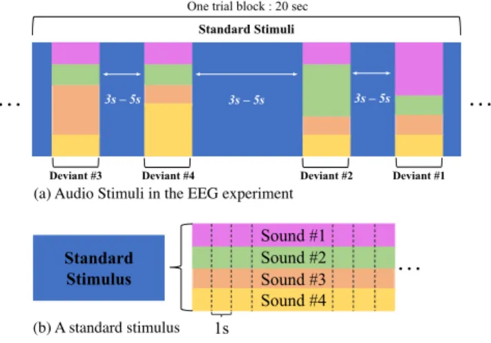
In each scene, the four sounds set forth in the respective columns of Table 1, each lasting one second, were mixed and used as that scene’s standard stimulus, which was played repetitively (Figure 1(b)). The intensity of the standard stimulus was controlled at 70 dB SPL. The deviant stimulus for each scene also comprised a mixture of the same four measured sounds, but one of them was increased by 15 dB SPL, i.e., to 85 dB SPL, while the other three sounds remained at the same level of intensity as the standard stimulus. The length of each deviant is one second. In this way, we created a competitive scenario of sounds, which is close to what we hear and experience in daily life. Between two consecutive deviant stimuli, the standard stimulus was played for at least three and up to five seconds. All stimuli were presented to the participants via loudspeakers.

A period of 20 seconds was set as a trial block (Figure 1). In each trial block, all four types of deviant stimuli were randomly included with equal probability of occurrence. To lessen the likelihood of the participants generating expectations about the audio stimuli, the total time of all deviants appearing in any trial block was controlled to not exceed 20%, i.e., four seconds or less. As previously stated, the interval between any two consecutive deviant stimuli was at least three seconds but not more than five seconds (Figure 1(a)). The order of the four deviant stimuli was also randomly arranged to reduce memory effects. Our paradigm design is shown in Figure 1. Each trial block was repeated for 45 times (i.e., there were 45 trials for each deviant) resulting in a total of 180 deviant trials per scene. The standard stimuli would be played for 10 seconds at the beginning of each scene – during which time EEG data was not recorded – so that they would form memory traces in the participants’ brains.

5.2 Participants and Device

Twenty healthy participants (10 females; 19-25 years old) with normal or corrected-to-normal vision were recruited for this experiment. None had a history of brain disease, drug use, or hearing problems (all participants could detect the variations of 15 dB SPL). There were two among twenty participants reported using iPhone. A 22-inch LCD monitor (1920x1080 pixels) was used to show videos, as explained below. Audio stimuli were presented via two loudspeakers (JS JY2009 2.0 ch), which were placed at a distance of 55 cm in front of the participants, at 30^◦to their left- and right-hand sides. A decibel meter was used to adjust the intensity of audio stimuli before each experiment started. We used Audacity (http://www.audacityteam.org/) to remove any blank before the onset of the sound in the soundtrack of each deviant.

(4)

MobileHCI ’19, October 1–4, 2019, Taipei, Taiwan Xun-Yi Huang, Fu-Yin Cherng, Jung-Tai King, and Wen-Chieh Lin

Scene 1: MRT Carriage Scene 2: Car Passenger Comparment

MRTbg MRT background Carbg Background in car

Walking Sounds of passengers walking Construction Construction outside the car CloseDoor Notification of closing door TurnSignal Notification of turn signal iPhone iPhone notification iPhone iPhone notification

Table 1: The table lists the auditory stimuli used in the MRT and Car scenes. Each scene contains four different stimuli. The same iPhone notification appeared in both scenes. The duration of each stimulus is one second.

3s – 5s

. . . . . .

One trial block : 20 sec Standard Stimuli

3s – 5s 3s – 5s

Deviant #3 Deviant #4 Deviant #2 Deviant #1

Sound #3 Sound #2 Sound #1

Sound #4 Standard

Stimulus

1s

. . . (a) Audio Stimuli in the EEG experiment

(b) A standard stimulus

Figure 1: (a) Timeline of the audio stimuli in the EEG experiment. Standard stimuli are repetitively played and all deviant stimuli are randomly scattered among the standard stimuli at the intervals of three to five seconds. For each deviant, there is one sound of which intensity is larger than the other three – the width of each color bar represents the intensity of each sound. The occurrence probability of each deviant is equal. (b) A standard stimulus is a mixture of four measured sounds and has a length of one second.

5.3 Procedure

Each participant was seated in a chair and was asked not to make large movements. The EEG headset was then put in place, and we began to explain the process of the whole experiment. The experiment started with the participant choosing a subtitled silent video from an on-screen menu of multiple options. All participants were asked to ignore auditory stimuli and pay attention only to the video during the experiment. As the video played, the participant would continuously hear auditory stimuli from the speakers. All participants were exposed to both the MRT and Car scenes, with a break of five minutes between scenes. It took each participant 30 to 40 minutes to complete both scenes. We counterbalanced the sequence in which the two scenes appeared, to avoid an ordering effect.

5.4 EEG Recording and Data Analysis

The EEG signals were recorded using a NeuroScan system and a non- invasive EEG cap with 32 Ag-AgCl electrodes, which all referred to both mastoid reference electrodes. For synchronizing a sound stimulus and its EEG recordings, we used the software Presentation

(https://www.neurobs.com) to program our experimental script.

Presentation would anchor and record the time markers of the onset time of each event in the EEG data. We can then analyze the EEG recordings based on these markers. All recorded data were filtered with a 1 Hz high-pass filter with a slope of 24 dB/oct, and a 30 Hz low-pass filter with a slope of 24 dB/oct off-line by using a Matlab toolbox, EEGLAB [7]. The purpose of high-pass and low- pass filtering is to remove unrelated physiological noises such as heartbeat and respiration [10, 33].

To allow us to analyze the effect of each deviant sound individ- ually, the EEG data were cut into a series of epochs. The epochs used for averaging were 600 ms long, starting 100 ms before and ending 500 ms after the stimulus onset. The 100 ms pre-stimulus period was set as a baseline. Before analyzing epochs, the EEG data from all 32 channels were processed with independent-component analysis (ICA) [27]. We selected those components affected by eye movement and blinking by visual inspection and then removed them. The number of components removed by ICA varied from 1% to 5%. After ICA-based artifact removal, all epochs with voltage variations exceeding 80µV were automatically rejected, since such voltage variations of physiological signals normally would not exceed 80µV. The voltage-variation-based rejection led to approxi- mately another 10% of raw data being removed from consideration.

After epoch rejection, at least 40 trials per participant remained for each deviant stimulus. Then, all epochs of the same stimuli (standard and deviant stimuli) were averaged, and the response to the standard stimuli was subtracted from the response to each type of deviant stimulus. However, we did not compute the difference wave for analysis because the subtraction could also reduce the signal-to-noise ratio (SNR) [19].

The time intervals for analyzing MMN and P3a were determined as follows. Firstly, we used the EEG data of all participants to compute the ERP of each deviant and identified the time points at which the peak value of each deviant’s ERP occurred. We call each time point in a deviant’s ERP a central time point. Secondly, we recorded the time points of all peaks for each trial of each deviant that occurred within the time interval of the central time point ± 50ms.

Thirdly, the minimal and maximal values of all time points among all trials of all deviants were set as the starting and ending points of the time interval. The time intervals obtained using the above steps for MMN and P3a were 90-230 ms and 155-310 ms, respectively.

The peak amplitudes for MMN and P3a were measured on the Cz channel from the most negative peak occurring around 90-230 ms and the most positive peak around 155-310 ms, respectively (Figure 2).

In the present study, we only utilized the Cz channel for MMN and P3a analysis. This was because previous studies [31] reported

(5)

EEG-based Measures of Auditory Saliency in a Complex Context MobileHCI ’19, October 1–4, 2019, Taipei, Taiwan

that MMN had a stable response at Cz, which is usually regarded as a representative channel of the MMN source with fewer artifacts of eye movement than other channels. In the statistical analysis, repeated-measures (RM) ANOVA was performed; Tukey’s method for multiple comparisons was then applied in post-hoc tests to determine the statistically significant differences. Mauchly’s test and Greenhouse-Geisser corrections were used to examine whether the data violated the assumption of sphericity.

5.5 Results of EEG Experiment

A one-way RM-ANOVA was used to determine if the measured sounds induced different MMN and P3a potentials. Mauchly’s test indicated that the assumption of sphericity was not violated except with the respect to the MMN results in the Car scene, the F values of which were corrected using Greenhouse-Geisser estimates of sphericity. We considered a critical p-value of 0.05 to determine statistically significant differences.

MRT Scene. Figure 2(a) shows the ERP curves evoked on the Cz channel during the MRT scene by each deviant stimulus and by the standard stimulus. The figure reveals that all deviants elicited a significantly larger negative deflection than the standard stimuli did, at around 150 ms after the stimulus onset. This was consistent with typical MMN responses. Moreover, the MMN amplitudes of the four measured sounds had statistically significant differences (main effect of deviant; F(4,1781)=54.40, p<.001). Following the occurrence of MMN, a positive ERP component P3a is generally elicited over the frontal-central area (electrode Cz) [35]. This P3a response was also clearly replicated in the present study, with the main effect of different deviants on P3a amplitude (F(4,1786)=88.65, p<.001), as indicated in Figure 2(a). The above results suggest that using MMN and P3a amplitudes to explore auditory saliency in complex contexts is feasible and that different stimuli can influence MMN and P3a amplitudes differently.

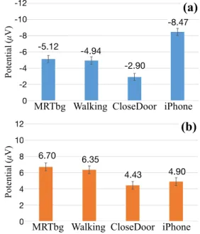
The MMN amplitude of each deviant is presented in Figure 3(a), from which a saliency ranking based on the deviants’ amplitudes could be deduced: iPhone > MRTbg ≥ Walking > CloseDoor. For this purpose, a larger MMN amplitude represents higher auditory saliency, and the notations “>” and “≥” denote that the level of saliency differs with or without statistical significance, respectively.

In other words, the p-value was <.05 in all post-hoc comparisons except MRTbg / Walking.

Figure 3(b) depicts the P3a amplitude of the four deviants. MRTbg and Walking exhibited larger P3a amplitudes than iPhone and Close- Door did: i.e., the ranking order of P3a amplitude was MRTbg ≥ Walking > iPhone ≥ CloseDoor. No statistically significant difference was found between MRTbg and Walking or between iPhone and CloseDoor. The different rankings of the amplitudes of P3a and MMN indicate that the same sound could have different levels of auditory saliency in the pre-attentive and post-attentive stages of auditory processing.

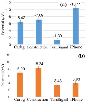
Car Scene. Figure 2(b) presents the ERP curves of all deviants in the Car scene. In the case of MMN, these curves generally exhibit typical responses (F(4,1763)=91.22, p<.001), the only exception being the TurnSignal sound, which did not differ significantly from the standard stimulus. There was a main effect of different deviants on P3a amplitude (F(4,1776)=74.02, p<.001). Interestingly, the P3a

Time (ms)

-100 0 100 200 300 400

Potential (7V)

-10

-5

0

5

10

Car (Cz)

Time (ms)

-100 0 100 200 300 400

Potential (7V)

-5

0

5

MRT (Cz)

Standard MRTbg Walking CloseDoor iPhone

Standard Carbg Construction TurnSignal iPhone

(a) (b)

Time (ms)

-100 0 100 200 300 400

Potential (7V)

-10

-5

0

5

10

Car (Cz)

Time (ms)

-100 0 100 200 300 400

Potential (7V)

-5

0

5

MRT (Cz)

(a) (b)

(a)

Time (ms)

-100 0 100 200 300 400

Potential (7V)

-10

-5

0

5

10

Car (Cz)

Time (ms)

-100 0 100 200 300 400

Potential (7V)

-5

0

5

MRT (Cz)

(a) (b)

Time (ms)

-100 0 100 200 300 400

Potential (7V)

-10

-5

0

5

10

Car (Cz)

Time (ms)

-100 0 100 200 300 400

Potential (7V)

-5

0

5

MRT (Cz)

(a) (b)

Time (ms)

-100 0 100 200 300 400

Potential (7V)

-10

-5

0

5

10

Car (Cz)

Time (ms)

-100 0 100 200 300 400

Potential (7V)

-5

0

5

MRT (Cz)

(a) (b)

Time (ms)

-100 0 100 200 300 400

Potential (7V)

-10

-5

0

5

10

Car (Cz)

Time (ms)

-100 0 100 200 300 400

Potential (7V)

-5

0

5

MRT (Cz)

(a) (b)

Standard MRTbg Walking CloseDoor iPhone

Time (ms)

-100 0 100 200 300 400

Potential (7V)

-10

-5

0

5

10

Car (Cz)

Time (ms)

-100 0 100 200 300 400

Potential (7V)

-5

0

5

MRT (Cz)

(a) (b)

Time (ms)

-100 0 100 200 300 400

Potential (7V)

-10

-5

0

5

10

Car (Cz)

Time (ms)

-100 0 100 200 300 400

Potential (7V)

-5

0

5

MRT (Cz)

(a) (b)

Standard Carbg Construction TurnSignal iPhone

(b)

Time (ms)

-100 0 100 200 300 400

Potential (7V)

-10

-5

0

5

10

Car (Cz)

Time (ms)

-100 0 100 200 300 400

Potential (7V)

-5

0

5

MRT (Cz)

(a) (b)

Time (ms)

-100 0 100 200 300 400

Potential (7V)

-10

-5

0

5

10

Car (Cz)

Time (ms)

-100 0 100 200 300 400

Potential (7V)

-5

0

5

MRT (Cz)

(a) (b)

Figure 2: MMN (90-230 ms) and P3a (155-310 ms) curves in the context of two sets of mixed audio stimuli, (a) MRT, and (b) Car. These ERP values are computed based on all valid trials by all participants. Y-axis represents the value of potential (µV). Time 0 in the x-axis indicates the start of each deviant.

0 2 4 6 8 10 12

dev1 dev3 dev2 dev4

-12 -10 -8 -6 -4 -2

0

dev1 dev3 dev2 dev4

-5.12 -4.94

-2.90

-8.47

(a) MMN Amplitude (MRT) (b) P3a Amplitude (MRT)

Potential (μV) Potential (μV)

MRTbg Walking CloseDoor iPhone MRTbg Walking CloseDoor iPhone

6.70 6.35

4.43 4.90

0 2 4 6 8 10 12

dev1 dev3 dev2 dev4

-12 -10 -8 -6 -4 -2

0

dev1 dev3 dev2 dev4

-5.12 -4.94

-2.90

-8.47

6.70 6.35

4.43 4.90

(a)

MRTbg Walking CloseDoor iPhone -5.12 -4.94

-2.90

-8.47 -12

-10 -8 -6 -4 -2 0

0 2 4 6 8 10 12

dev1 dev3 dev2 dev4

-12

-10

-8

-6

-4

-2

0

dev1 dev3 dev2 dev4

-5.12 -4.94

-2.90

-8.47

6.70 6.35

4.43 4.90

0 2 4 6 8 10 12

dev1 dev3 dev2 dev4

-12

-10

-8

-6

-4

-2

0

dev1 dev3 dev2 dev4

-5.12 -4.94

-2.90

-8.47

6.70 6.35

4.43 4.90

12 10 8 6 4 2 0

0 2 4 6 8 10 12

dev1 dev3 dev2 dev4

-12 -10 -8 -6 -4 -2

0

dev1 dev3 dev2 dev4

-5.12 -4.94

-2.90

-8.47

6.70 6.35

4.43 4.90

0 2 4 6 8 10 12

dev1 dev3 dev2 dev4

-12 -10 -8 -6 -4 -2

0

dev1 dev3 dev2 dev4

-5.12 -4.94

-2.90

-8.47

6.70 6.35

4.43 4.90

(b)

MRTbg Walking CloseDoor iPhone 6.70 6.35

4.43 4.90

-12 -10 -8 -6 -4 -2

0

dev1 dev2 dev3 dev4

0 2 4 6 8 10 12

dev1 dev2 dev3 dev4

(a) MMN Amplitude (Car) (b) P3a Amplitude (Car)

Carbg Construction TurnSignal iPhone Carbg Construction TurnSignal iPhone

-6.42 -7.09

-1.30

-10.41

6.90

8.34

3.43 3.93

-12 -10 -8 -6 -4 -2

0

dev1 dev2 dev3 dev4

0 2 4 6 8 10 12

dev1 dev2 dev3 dev4

-6.42 -7.09

-1.30

-10.41

6.90

8.34

3.43 3.93

-12 -10 -8 -6 -4 -2

0

dev1 dev2 dev3 dev4

0 2 4 6 8 10 12

dev1 dev2 dev3 dev4

-6.42 -7.09

-1.30

-10.41

6.90

8.34

3.43 3.93

-12 -10 -8 -6 -4 -2

0

dev1 dev2 dev3 dev4

0 2 4 6 8 10 12

dev1 dev2 dev3 dev4

-6.42 -7.09

-1.30

-10.41

6.90

8.34

3.43 3.93

-12 -10 -8 -6 -4 -2 0

(a)

(b)

12 10 8 6 4 2 0

Carbg Construction TurnSignal iPhone

Carbg Construction TurnSignal iPhone -6.42 -7.09

-1.30

-10.41

6.90

8.34

3.43 3.93

0 2 4 6 8 10 12

dev1 dev3 dev2 dev4

-12

-10

-8

-6

-4

-2

0

dev1 dev3 dev2 dev4

-5.12 -4.94

-2.90

-8.47

6.70 6.35

4.43 4.90

0 2 4 6 8 10 12

dev1 dev3 dev2 dev4

-12

-10

-8

-6

-4

-2

0

dev1 dev3 dev2 dev4

-5.12 -4.94

-2.90

-8.47

6.70 6.35

4.43 4.90

0 2 4 6 8 10 12

dev1 dev3 dev2 dev4

-12

-10

-8

-6

-4

-2

0

dev1 dev3 dev2 dev4

-5.12 -4.94

-2.90

-8.47

6.70 6.35

4.43 4.90

0 2 4 6 8 10 12

dev1 dev3 dev2 dev4

-12

-10

-8

-6

-4

-2

0

dev1 dev3 dev2 dev4

-5.12 -4.94

-2.90

-8.47

6.70 6.35

4.43 4.90

0 2 4 6 8 10 12

dev1 dev3 dev2 dev4

-12

-10

-8

-6

-4

-2

0

dev1 dev3 dev2 dev4

-5.12 -4.94

-2.90

-8.47

6.70 6.35

4.43 4.90

0 2 4 6 8 10 12

dev1 dev3 dev2 dev4

-12

-10

-8

-6

-4

-2

0

dev1 dev3 dev2 dev4

-5.12 -4.94

-2.90

-8.47

6.70 6.35

4.43 4.90

Figure 3: (a) and (b) are the MMN and P3a amplitudes, respectively, of the four deviant sounds in the MRT context. The error bars show the standard errors.

of the TurnSignal sound could be elicited without the premise of evoked MMN response. Figure 4(a) reveals the ranking of the deviants based on their MMN amplitudes: iPhone > Construction

≥ Carbg > TurnSignal, where p values were <.05 in all post-hoc comparisons except Construction / Carbg. Figure 4(b) shows the ranking order of P3a amplitude as Construction > Carbg > iPhone

≥ TurnSignal. No statistically significant difference was found between Turn Signal and iPhone.

This result shows, first, that our method is practicable not only in the context of one scene, but could also reveal the different influences of different scenes. Second, in parallel to the results of the MRT scene, the iPhone sound had the highest level of aware- ness (MMN) for people in the pre-attentive stage, but caused lower levels of attention shifting (P3a) while the processing was in the