適用於光池加速光線追蹤繪圖之多核心處理器硬體架構設計

(1)

國立臺灣大學電機資訊學院電子工程學研究所碩士論文

Graduate Institute of Electrics Engineering

College of Electrical Engineering and Computer Science National Taiwan University

Master Thesis

適用於光池加速光線追蹤繪圖之多核心處理器硬體架構設計

Ray-Pool Based Configurable Multiprocessor Design for Ray Tracing

謝明倫 Ming-Lun Hsieh

指導教授：簡韶逸博士 Advisor: Shao-Yi Chien, Ph.D.

中華民國 104 年 9 月

September 2015

(2)

(3)

(4)

誌謝

這篇論文的完成有賴於眾人的協助，尤其本篇論文算是合作計畫中的子題延伸發展而來。過往學者們的研究成果、技術、方法也都是十分重要的基石；研究過程中的老師、學長姊以及夥伴們亦是直接的助力。在此感謝諸位直接或間接的種種幫助。

首先要感謝我的指導教授簡韶逸博士。在碩士班的生涯裡，老師總是悉心瞭解研究的進展與遭遇到的難關，盡力的為學生思考可能的癥結，輔以自身經驗並為學生尋找資源出路。永遠難忘半夜兩點寄信，老師竟能在四點立即回覆。研究過程中偶遇挫折，也是靠老師帶領轉個彎思考，進入新方向。論文是一篇完整的故事，需要有邏輯的因果順序和定位，在埋頭苦做時有賴老師引領注意全貌。

接著感謝光池小組的團隊：宥融學長、彥瑜學長、哲堯同學。萬事起頭難，

初步的構想與前進的方向左右了結果好壞甚大。光池的雛型來自於兩位學長的洞見，其後才有筆者的實現討論。也特別感謝宥融學長從我任專題生以來一路的引導與指點，身在國外亦不忘關心學弟的近況，指出了許多筆者忽略了的盲點。

感謝裕盛學長如兄長般親切的協助。處理器的研究源遠而深究精細，許多看不通透的實作細節，都是在與學長討論後方得以釐清。眾多開發資源的統整利用也是裕盛學長的強項，為實驗效率增色不少。

也感謝實驗室內的夥伴們，一個組織的順利運作是構築在眾人的齊心合作上，每個人都有各自扮演的角色。另外，實驗室的大家也是心靈支持上的好夥伴。經常的聚餐出遊聊天吐苦水，是平復緊張心情的最好充電站。

聯發科計畫中的各長輩、前輩們也是一大助力，提點該如何用業界的眼光做好事前的計畫。對此我還有許多進步的空間，但很高興這開拓了我的眼界。

最後我要感謝一直以來支持我的家人，家人的信賴與陪伴永遠是最強而有力的靠山。雖然對於我在研究什麼頂多僅一知半解，但永遠為此加油打氣，也讓我能毫無後顧之憂地專心在研究上。

(5)

摘要

逼真的電腦繪圖技術如今已是日常生活中的一部份。但人們依舊追求更高端更真實的繪圖技術，傳統的柵格化投影技術已不再能滿足此需求。光線追蹤等物理擬真新渲染技術被看好具備十足的潛力，但仍有技術問題尚待克服：高運算量與高動態分歧。本篇論文提出一種新的光線追蹤加速硬體架構，期待克服以上問題，進而涉足即時光線追蹤渲染的境界。

光線追蹤相較傳統做法多了光線生成、空間追蹤、交點測試等運算步驟。其中，每次光線可能出現偏折散射時，會指數增長出更多需要追蹤的新目標；甚至更細膩的繪圖上還需要大量取樣機率分布，如：路徑追蹤演算法。更甚者，這些光線還要與數十萬的三角形物件進行交點測試，進而開啟了加速結構的研究大門。此外，這些目標光線隨空間的行進將越來越發散，難以用現今的通用圖形處理器來平行加速。每次偏折都帶來運算上的分歧，使得快取記憶在讀取上失去區域性的好處，拖慢了整體的速度。

本論文所提出了「光池加速光線追蹤繪圖器」的新硬體加速架構，以克服這些問題。本架構亦參考相關的先前文獻如 SGRT、PowerVR GR6500 等，將整個運算過程分為兩部分：專責空間追蹤和交點測試的硬體追蹤單元，以及保留了可程式化能力的渲染器單元。本文的光池加速架構希望能透過介於其間的兩個光池，重分配調和上述兩運算單元的工作，進而達到高效率運算的好處。藉由光池的重整與抽象化，運算單元將可更獨立，各自進行所需的高速運算。

其中，本論文針對渲染運算單元，設計了一個參數化且易於重組的多核心處理器。其特色在於：把運算分組為功能單元，各功能單元都能輕易的在此處理器的設計上添減、方便擴充與客製化所需的功能。此處理器經邏輯合成驗證，在 TSMC 40 奈米製程下能以 1GHz 的時頻運作，並附帶一個近乎時間精確的軟體模擬器供開發測試。

經模擬實驗，此一光池加速光線追蹤繪圖器可以達到每秒處理一億條光線 (100Mrays/s)的最高效能。該系統包含四組運算單元(每組含 8 核心 8 套資料)、

108 千位元組(KB)的光池與特化硬體追蹤單元(具每秒一億筆空間追蹤能力)。此一系統得以即時渲染基本光線(primary ray only)於高畫質(HD, 720p)解析度上，或是即時渲染五層懷式演算法反射光於傳統解析度(480p)上。

(6)

Abstract

Realistic image synthesis is now everywhere in our daily lives. People pursue new experience of much more realistic of displays than traditional rasterization-based method.

Ray tracing, as one of the physically-based rendering methods, is provided as a candidate for next generation of image synthesis. However, it comes with problems about large scale computation and diversity to be conquered. In this thesis, a simple but complete hardware for real time ray tracing is proposed, trying to overcome these problem.

Ray tracing requires additional computation of ray generation, traversal and intersection test with objects. These rays may grow exponentially as each bounce of reflection and refraction or even samples of specific distribution for path tracing. Meanwhile, there are hundreds of thousands of triangles to test. It starts the researches of accelerating data structures for them. On the other side, rays become more and more diverse as they traverse deeper. It is not compatible to the programming model of current

GPGPUs. The divergence of data access in ray tracing causes the performance drop by cache evictions.

Ray-pool based ray tracer (in short as RPRT) is then proposed. As a hardware architecture to solve these problem. Like previous work such as SGRT and PowerVR GR6500, RPRT separates the process of traversal and intersection to a specialized hardware while keeping the programmability in shader. RPRT tries to make these two computational units co-works efficiently by adding two pool between them. By the arrangement and virtualization of two pools, the two computational unit can work simultaneously and independently.

In this system, a configurable multiprocessor is designed as the need for shader. It is easy to configure and easy to extend for different applications with customized ALUs.

It comes with a near cycle accurate simulator verified by hardware implementation after logic synthesis. It works at the clock rate of 1GHz under the TSMC 40 nm process.

By experiments on RPRT system, it can reaches 100Mrays/s of performance under the configuration of 4 compute units multiprocessor, 8 warps 8 cores in each CU, 108KB pools, and an ASIC traverser with ability of about 100Mtraversal/s. This result reveals the possibility of real-time hardware ray tracing at 720p with basic effects by primary rays and 480p by the traversal depth of 5.

(7)

List of Figures

Figure 1.1 The concept of Whitted style ray tracing ... 2

Figure 1.2 Difference between rasterization and ray tracing ... 3

Figure 3.1 Main concept of RPRT ... 9

Figure 3.2 System architecture of RPRT ... 9

Figure 3.3 Block diagram of software simulator ... 11

Figure 4.1 Instruction routine ... 14

Figure 4.2 Data routine ... 14

Figure 4.3 Pipeline stages ... 15

Figure 4.4 Simulator model ... 16

Figure 4.5 A detailed snapshot of operating flow hiding memory latency ... 17

Figure 4.6 Latency and pipeline configuration illustration ... 19

Figure 4.7 Simulating non-blocking cache ... 20

Figure 4.8 Illustration of instruction generating tool ... 22

Figure 4.9 Two modes of simulation ... 22

Figure 4.10 Local ray memory in RayALU ... 23

Figure 5.1 Target scene: conference ... 26

Figure 5.2 Three kinds of kernel ... 27

Figure 5.3 Kernel choice policy by controller ... 29

Figure 5.4 Window effect avoidance in kernel launch policy ... 30

Figure 5.5 Performance of different configurations (single CU) ... 34

Figure 5.6 Normalized Performance of different configurations (single CU)... 34

Figure 5.7 ALU utilization rate in different configuration (32 contents) ... 35

Figure 5.8 ALU utilization rate for different contents (4 cores) ... 36

Figure 5.9 Average waiting traffic of ALUs (32 contents) ... 36

Figure 5.10 Performance of multiple CUs (32 contents)... 39

Figure 5.11 Normalized Performance of multiple CUs (32 contents) ... 39

Figure 5.12 Performance of multiple CUs (32 contents)... 40

Figure 5.13 Normalized Performance of multiple CUs (64 contents) ... 40

Figure 5.14 Comparison of ALU utilization rate in multiple CUs ... 41

Figure 5.15 Multiple CUs versus multiple contents in performance ... 41

Figure 5.16 New kernel choice policy for large scale configuration ... 42

Figure 5.17 Comparison of different kernel choice policy on 4 CUs 64 contents ... 43

Figure 5.18 Comparison of different policy with normalized performance on 4 CUs 64 contents ... 44

Figure 6.1 Architecture of multiprocessor implementation ... 45

(10)

Figure 6.2 Functional pipelines for data routine ... 46

Figure 6.3 Functional pipelines for instruction routine ... 47

Figure 6.4 Tables for dispatcher arbiting ... 48

Figure 7.1 An example of changing kernel choice policy ... 53

(11)

List of Tables

Table 1.1: Performance requirements for different resolutions ... 4

Table 2.1: Fast comparison of hardware ray tracer ... 7

Table 4.1: Latency and pipeline configuration of ALUs ... 18

Table 5.1: Number of instructions in different kernel ... 28

Table 5.2: Effect to pools of different kernels ... 28

Table 5.3: Results of single CU with 16 contents ... 31

Table 5.6: Results of 2 CUs with 32 contents ... 37

Table 5.10: Results of 4 CUs with 64 contents by new policy ... 43

Table 6.1: Area report ... 49

Table 7.1: Quick example in kernel choice policy ... 53

(12)

Chapter 1 Introduction

Realistic image synthesis [1] is now everywhere in our daily lives, from gaming, mov- ies, designs and user interfaces. People pursue more and more realistic experience of displays without stop. However, traditional rasterization-based method has its limitation for further physically-correct effect in rendering. Ray tracing, as one of the physically- based rendering [2] methods, is provided as a candidate for next generation of image synthesis. But it comes with new problems to be fixed.

1.1 Physically-Based Rendering

Physically-based rendering is the process of generating images by simulating the transportation of lights captured by virtual cameras in the field of computer graphics. For this reason, researchers try to build different models imitating the physical mechanism of light transportation and interaction with environment.

1.1.1 Rendering Equation

Rendering equation [3] is proposed by Kajiya as a general equation. It solves the relationship between scene geometry, materials and observer.

𝐿_𝑜(𝑥, 𝜔_𝑜) = 𝐿_𝑒(𝑥, 𝜔_𝑜) + ∫ 𝑓(𝑥, 𝜔_𝑜, 𝜔_𝑖) ∙ 𝐿_𝑖(𝑥, 𝜔_𝑖) ∙ |𝑐𝑜𝑠𝜃_𝑖| ∙ 𝑑𝜔_𝑖

Ω

Symbol x represents the surface point, ωi, ωo are incident and outgoing solid angles of light, L means radiance and f is bidirectional reflectance distribution function denot- ing characteristics of surface material.

But in the concern of computation practicing, there are various simplified models and techniques are proposed. One of the most famous and simplest method is Whitted style ray tracing [4].

1.1.2 Whitted Style Ray Tracing

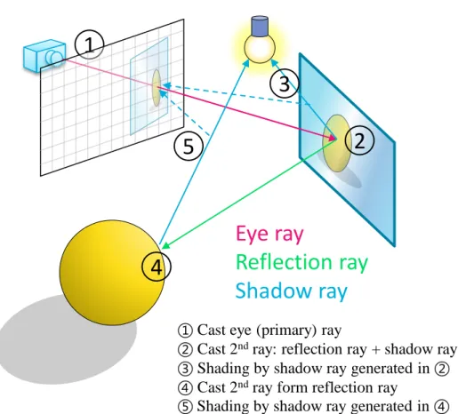
Whitted style ray tracing is based on the basic concept of rays as straight lines. Rays split and turn at surfaces of objects following Snell’s law as reflection rays and refraction rays. The computation process starts from tracing the rays entering observer’s eye

(13)

by shooting “rays” passing through pixels on scene frame. Each time these rays hit an object, it generates the secondary ray of reflection, refraction and a shadow testing ray for energy accumulation. The ray traversal and scatter steps run recursively.

Shadow rays are a special kind of rays. It calculates the energy from every light source to the surface. This energy is back-accumulated to corresponding pixel as color and intensity. If shadow rays are blocked by other objects, this accumulating process is blocked, too, making a dark point as shadow. An illustration of these steps is shown in Figure 1.1.

Figure 1.1 The concept of Whitted style ray tracing

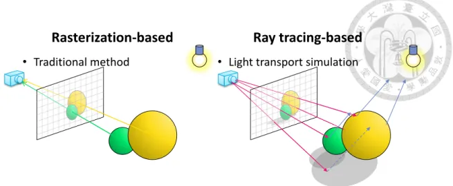
Figure 1.2 shows the difference of traditional rasterization-based method and Whit- ted style ray tracing.

1 Eye ray

Reflection ray Shadow ray

2

4 3 5

① Cast eye (primary) ray

② Cast 2

^nd

ray: reflection ray + shadow ray

③ Shading by shadow ray generated in ②

④ Cast 2

^nd

ray form reflection ray

⑤ Shading by shadow ray generated in ④

(14)

Figure 1.2 Difference between rasterization and ray tracing

1.2 Limitations of Current GPUs for Ray Tracing

Though ray tracing brings the benefits of realistic synthesis, it comes with two tough topic: huge computation process and diversity in both control and data access.

Firstly, it requires lots of additional computation of rays, ray traversal and intersection test with objects. For traditional method, objects are projected to view plane directly at the cost of about number of objects multiplies complexity of objects. But ray tracing requires searching for each primary rays at an exponential growth of search depth. And for each search, it takes intersection test with objects, acting as another huge multiplier. Though there are many accelerating data structures to reduce the testing process, it still have much more computation requirement than traditional one.

On the other side, rays become more and more diverse as they traverse deeper. It is not compatible to the programming model of SIMD (single instructions multiple data) multiprocessors. It requires at least doing rearrangement for each braches, breaking re- cursive process to iterative process or taking the advantages of SIMT (single instructions multiple threads) multiprocessor. Though these solve the control problem, it still suffer from divergence in data access.

Caches improves performance by the assumption of temporal locality and spatial locality of computation. But the divergence of data access in ray tracing may break this assumption, making more cache evictions.

1.3 Motivation and Target

Because of these limitations on traditional GPGPUs (general-purpose computing on graphics processing units), many application specific hardware are proposed for ray tracing. Especially, real time ray tracing is hot topic for users seeking for realistic ren-

Rasterization-based

• Traditional method

Ray tracing-based

• Light transport simulation

(15)

dering on their devices. This thesis also tries to accelerate this process achieving efficient and real time ray tracing.

For real time ray tracing, the performance requirement for different resolutions are showed in Table 1.1. Proposed system targets the performance at about 100 Mrays/s, ca- pable for real time ray tracing at 720p with basic rendering effects by primary rays and 480p with more effects by the traversal depth of 5.

Table 1.1: Performance requirements for different resolutions

Types Basic rendering

(Primary rays)

Typical effects (Traverse at depth of 5)

480p, 30fps

18.4 Mrays/s ~92.2Mrays/s

480p, 60fps

36.9Mrays/s ~184.3Mrays/s

720p, 30fps

720p, 60fps

To solve the problems mentioned above in section 1.2 , we come up with the idea of ray-pool based ray tracing architecture. By gathering rays as pools, basic rearrangement of rays can be done inside these pools. Moderates the problem of divergence. This thesis is an implementation of such ray-pool based ray tracer system.

However, this system requires a multiprocessor that is easy to transplant and maintain for our ray-pool base system while is configurable when taking experiments. So we build up such configurable multiprocessor, as another important part discussed in this thesis.

1.4 Thesis Organization

The chapters bellow are arranged as following. Chapter 2 introduces and reviews some previous ray tracing engines with fast comparison. Chapter 3 gives an overview and concepts of proposed ray-pool based ray tracing system. Chapter 4 focuses on the proposed configurable multiprocessor for this system. Chapter 5 reveals the methodology of simulation and experiments for performance of the system. Chapter 6 describes the hardware implementation for multiprocessor to show the feasibility. Then Chapter 7 discusses about the non-simulated parts and future works. While conclusion of this thesis is offered in Chapter 8 .

(16)

Chapter 2 Previous Work

In this chapter, we introduce several hardware accelerated ray tracing techniques or devices. In section 2.4 , we give a fast comparison of these work and make a short summary from them.

2.1 Ray Core

RayCore [5] is a hardware ASIC (application-specific integrated circuit) for ray tracing on mobile devices. Though it says RayCore architecture is based on MIMD (multiple instruction multiple data)-based ray tracing architecture, it also reveals that RayCore is made as fixed-function units instead of programmable units. We think maybe we can classify it as MIMD-inspired ASIC since RayCore consults ideas from MIMD architecture to make its function pipeline.

It has the performance of 193Mrays and claims able to render HD 720p at 56 FPS.

RayCore is based on Whitted style ray tracing with SAH kd-tree as the acceleration data structure. It supports dynamic scenes construction, building SAH kd-tree for 64K triangles within 20 ms.

RayCore is composed of six ray tracing unit (RTU) and one tree building unit (TBU). Targets for 28 nm process with the area of 18(RTU) + 1.6(TBU) mm² and the clock rate at 500MHz. It is a power efficient work with the power consumption at about 1 W.

RayCore is a complete work supporting OpenGL ES 1.1-like API and has been verified on FPGA board.

2.2 SGRT

SGRT is the short of Samsung reconfigurable GPU based on ray tracing [6]. SGRT is a mobile solution for ray tracing based on two parts: GPU and ASIC for T&I (traversal and intersection). A typical devices has 4 SGRT cores, each single SGRT core consists of a SRP (Samsung Reconfigurable Processor) and a T&I unit.

SRP is a MIMD mobile GPU with theoretical peak performance of 72.5 GFLOPS (giga floating point operations per second) per core at 1 GHz clock frequency and 2.9 mm² at 65 nm process. It comes with a very long instruction word engine and a coarse- grained reconfigurable array of ALUs.

(17)

A T&I unit [7] consists of a ray dispatch unit, 4 traversal units, and an intersection unit. T&I unit in SGRT selects the BVH tree as the acceleration structure. SGRT proposed the parallel pipelined traversal unit architecture to further accelerate the traversing process.

The 4-core SGRT has the performance of 184 Mrays/s on conference scene and claims able to render FHD 1080p at 34 FPS. SGRT does not support dynamic scenes construction on it. Only static scene is tested and BVH trees are built by CPU. Though it seems weaker than RayCore in performance, it remains the programmable GPU part.

Their processes are different, too. SGRT targets at a more previous process of 65 nm with the area of 25 mm² for 4 cores. The clock rate is 500MHz for T&U and 1GHz for SRP. SGRT is also verified on FPGA board.

2.3 PowerVR GR6500

PowerVR GR6500 [8] is a coming device designed by Imagination Technologies. It is a GPU embedded with ray tracing hardware. But there is no complete official datasheet available now. Only little information is revealed.

It claims having the ability of rendering at 300Mrays/s with 100M dynamic triangles. GR6500 supports hybrid rendering (rasterization + ray tracing) and dynamic scene construction by a scene hierarchy generator. Their ray tracing unit is also a fixed-function.

Besides ray tracing unit, there is a ray tracing data master managing transmission of ray intersection data to the main scheduler, in preparation for shaders to run. On the other hand, GR6500 is yet a GPU with 128 ALU cores running at 600MHz with 150 GFLOPS.

2.4 Short Summary

A fast comparison of these works is shown in Table 2.1. From these work, it seems that making a special function unit handling ray traversal and intersection is a more efficient way in ray tracing. And there is a trade-off of programmability with efficiency as fixed function about shaders. From SGRT and GR6500, we know that the cooperation of shaders and traversers is an important issue.

Our work is a trial of another architecture. We propose a simple but complete system prototype with approaching performance with those state-of-the-art works. In comparison, GTX680 is an extreme example of a pure general-purposed computation machine. Though it has lots of resource of FLOPS and bandwidth, it only has little ad- vantage over others when they scale up. Our ray-pool based system is also a simple but efficient solution for ray tracing. The proposed system only requires fewer computation

(18)

resource while keeping the programmability and performance for ray tracing.

Table 2.1: Fast comparison of hardware ray tracer

GTX680 [9]

Optix [10] RayCore SGRT PowerVR

GR6500 Ours

Year

2013 2014 2013 2015 2015

Process

28nm 28nm 65nm 28nm 40nm

Type

GPU ASIC GPU+ASIC GPU+ASIC GPU+ASIC

Clock

1GHz 500MHz ASIC:500M

MIMD:1G 600MHz 1GHz

N Cores

1536 1+4 4 128 8x4+?

GFLOPS

3000 72.5x4 150 8x4

BW(GB/s)

192.2 8

Area

294 18+1.6 25 16

Mrays/s

(Primary)

432 193 184 300 100

(19)

Chapter 3 System Overview

In this chapter we give a fast description of proposed “ray-pool based ray tracing system” (in short as RPRT).

3.1 Main Concept

For real time ray tracing hardware, how to divides algorithm to programs and ASIC while keeping high efficient cooperation of them is an important topic. Having a look at previous work, most of them come with a ray traversal ASIC and many of them pre- serve some parts of programmable processor.

We also adopt this idea to divide the whole process into processors and special ACIS. Since there are many different algorithms for ray tracing, it is better to keep some programmable parts for different application. Also, a programmable processor can share the computation of other applications besides ray tracing if needed.

Meanwhile, through different types of ray tracing algorithm, many of them have the similar process of finding ray-triangle intersection. Showing this intersection process is an important efficiency topic. So we leave a special ASIC to accelerate this process while keeping the supportability of different algorithm.

To make these two part cooperate efficiently, we insert two pools between them.

By the arrangement and virtualization of two pools, the two computational unit can work simultaneously and independently (little suffering from stalls by other).

(20)

Figure 3.1 Main concept of RPRT

3.2 System Architecture

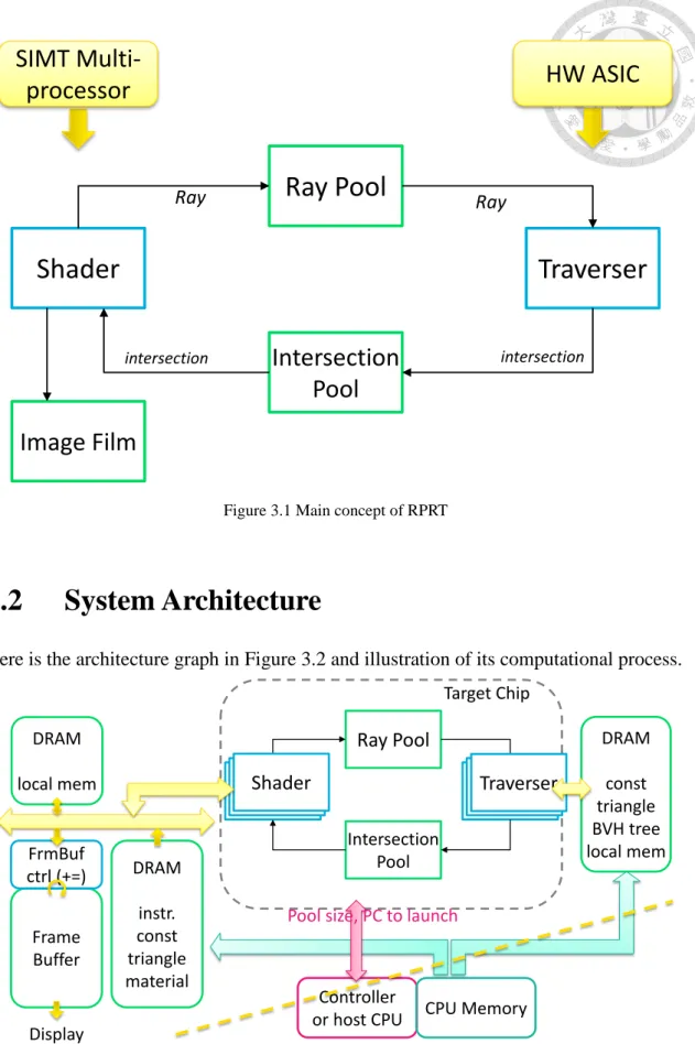
Here is the architecture graph in Figure 3.2 and illustration of its computational process.

Figure 3.2 System architecture of RPRT

Our system can be view as a new graphics card. Firstly, host CPU move instructions (kernel codes) and related data from main memory to DRAMs of our system. After contents are ready, the host CPU send a starting signal with kernel code address to

Shader Traverser

Ray Pool

Intersection Pool Image Film

Ray Ray

intersection intersection

SIMT Multi-

processor HW ASIC

Target Chip

DRAM instr.

const triangle material

Controller or host CPU

DRAM const triangle BVH tree local mem

Frame Buffer

Shader Traversor

Ray Pool

Intersection FrmBuf Pool

ctrl (+=) DRAM local mem

Display

CPU Memory Pool size, PC to launch

Shader Shader Traversor Traverser

(21)

launch. Shader then starts running the according kernel. At the end of kernel, the rays generated are pushed into Ray Pool and trigger the task of Traverser.

After the end of kernel, the Controller decides the next kernel to launch based on the size of two pools. That Controller may be the host CPU or an on-board embedded CPU. This kernel choice process is practiced many times to complete a single frame.

As for memory system, since the two computational unit (Shader and Traverser) are working separately, we use two independent memory spaces and ports for them.

Only triangle data is duplicated for both of them.

Accelerating data structure for traversal such as BVH tree needs to be pre-com- puted in our current system. And is moved to Traverser’s memory in advanced. But such process still can be done by cooperation between Shader kernel and host CPU furtherly.

3.3 Shader (Configurable Multiprocessor)

Our Shader here is a self-designed configurable multiprocessor. And this is the main contribution of this paper. There are more details discussed in Chapter 4 .

Since there are little open resources of general purpose multiprocessor that can be easily configured and linked with self-defined special units in both software simulator and hardware implementation currently, we make one by ourselves. Our configurable multiprocessor is a CUDA-like SIMT (single instruction multiple threads) processor which have the benefits of easier to program [11] and able to hide memory latency.

Our configurable multiprocessor can be changed in numbers of threads (cores), warps and compute units. And is written with many parameters in both simulator and hardware Verilog implementation, such as pipeline stages of ALUs and the combination of ALUs. It is also easy to plug-in self-defined function units by following simple interfaces.

Followings are the configuration of multiprocessor used in proposed typical RPRT.

It has 4 compute units, each contains an 8 cores ALU set with 8 warps, 4KB instruction cache, 8KB data cache and 16KB specialized local memory for ray tracing.

3.4 Ray Traverser

Details of ray traverser is not the main focus of this thesis. There are lots of research studying about hardware traverser. Many of them are compatible with our ray-pool based ray tracing system. We only assume that this traverser having the nearly ability (both throughput and latency) with our Shader at about 100Mrays per second.

Ray Traverser is a hardware ASIC designed for traversal and intersection. Tra- versal is the step to find which triangle may on the way of the target ray. Recent traversal step arranges triangles into data structure like BVH (bounding volume hierarchy)

(22)

[12] [13] tree according to space locality. The main process is hardware accelerated parallel tree traversal. As for intersection, it is the step to certainly calculate the intersection point of target ray and candidate triangle suggested by traversal step.

Take Chang’s work [14] for example, it is complete system for ray tracing. It is designed in cell-based design flow under UMC 90nm process with about 9 mm² core area, operating at the clock rate of 125MHz. It has the capability of 125 M traversals and 62.5 M intersections per second which is suitable for our requirement. It traversing the BVH tree with packets of 64 rays. It is also balanced with our Shader in the typical configuration of 8 cores and 8 warps (a batch of 64 contents per compute unit).

3.5 Software Simulation

We build up the simulation environment on SystemC version 2.3.0. It is mainly designed as a component-assembly model with approximated timing accuracy in functionality. It is near cycle accurate in Shader part while approximated timed in other parts. As for communication between modules, transportation inside our chip (Shader, Traverser and two pools) is approximate-timed calculated by bandwidth. The memory access from Shader is approximate-timed, too. But the other communications are un-timed in our simulator, such as host CPU and host memory. More details can be found in section 5.2 .

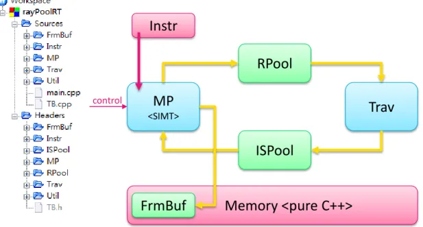
Figure 3.3 Block diagram of software simulator

Figure 3.3 illustrates the main blocks of our simulator. The MP, Trav, RPool and ISPool parts are our SystemC modules and functions of configurable multiprocessor (Shader), ray traverser, ray pool and intersection pool respectively. Functions of kernel control for host CPU are written in TB.cpp/h. Benchmark data and self-made instruction

MP

<SIMT>

Trav

RPool

ISPool

Memory <pure C++>

FrmBuf Instr

control

(23)

generating tools are handled in Instr.

We do all the measurements and optimize our system based on this simulator and verified the Shader part by Verilog implementation. Experiments details are showed in Chapter 5 .

3.6 Hardware Implementation

We implement our configurable multiprocessor by Verilog HDL and verified by logic synthesis using the tool of Synopsis Design Compiler with TSMC 40nm process. The designed working frequency is 1 GHz. And the cell area reported by synthesis tool is 0.537 mm² for single compute unit under the configuration of 4 cores and 4 warps.

More information is showed in Chapter 6 .

(24)

Chapter 4 Configurable Multiprocessor Simula- tion

In this chapter we propose a simple but complete SIMT multiprocessor, which is the main contribution in this work.

The followings are some specifications of our processor. It runs at the clock rate of 1 GHz with 4 stages pipeline. Using 64-bit self-defined instruction and 32-bit width data (both integer and single precision floating point data). The number of cores and warps are configurable ranging from 1 to 32 as the exponent of 2 in each compute unit (streaming multiprocessor in CUDA). Each thread has 16 general registers. The number of compute unit is also configurable ranging from 1 to 4. Each compute unit possess an 8KB L1 data cache and a 4KB L1 instruction cache. Both two caches are 2 way set as- sociative.

The originally framework of this processor is established by Yu-Sheng Lin and designed as a GPGPU (general-purpose GPU). He draws up the basic architecture by re- ferring to a paper [15] about GPGPU-SIM [16]. Our processor further extend Lin’s work making it more configurable, accurate and concrete. It’s near cycle accurate now, and can be verified by hardware implementation.

As a result, our processor is a CUDA-like SIMT multiprocessor. We have very similar idea of “threads, warps, blocks, kernels, SMs (we use the word ‘compute units’

here)” as CUDA programming model [17].

4.1 Operating Flow

The operations of our processor are spilt into two part (instruction routine and data routine) with a few step. We group a fixed amount of operation threads (typically: 8) into a warp as the basic unit in our operation flow. To make things easy, we only discuss the operating flow of a single warp in section 4.1. And later discuss the relationship between warps in section 4.2.

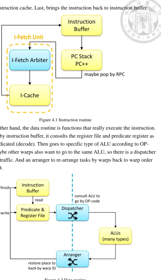
The instruction routine is functions that request a correct instruction to run. First, instruction buffer updates its state and starts instruction request. Second, it finds the top entry of PC (program counter) stack and increase the PC to next instruction address.

Then, send a request to instruction fetch unit. The chosen request by arbiter is able to

(25)

consult the instruction cache. Last, brings the instruction back to instruction buffer.

Figure 4.1 Instruction routine

On the other hand, the data routine is functions that really execute the instruction.

Also starting by instruction buffer, it consults the register file and predicate register as instruction indicated (decode). Then goes to specific type of ALU according to OP- code. But maybe other warps also want to go to the same ALU, so there is a dispatcher to handle the traffic. And an arranger to re-arrange tasks by warps back to warp order using warp ID.

Figure 4.2 Data routine

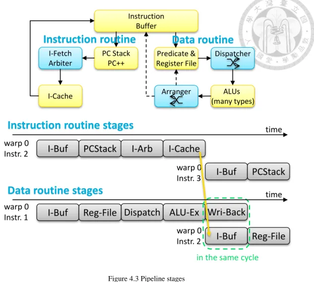
By means of real hardware implementation, taking logic and flip-flop delays into concern, we have the following pipeline stages: IBuf, PCStack, IArb, ICache, RegFile, Dispatch, ALUEx, WriBack.

Instruction Buffer

PC Stack PC++

maybe pop by RPC

I-Fetch Arbiter

I-Cache

Instruction Buffer

Predicate &

Register File

ALUs (many types) Dispatcher

Arranger

read consult ALU to

go by OP-code

restore place to back by warp ID write

finish

(26)

Figure 4.3 Pipeline stages

The WriBack stage and next IBuf stage can be done in the same cycle by tracing the execution state in instruction buffer properly. In case that both two routines have not stalls (chosen by arbiter, cache hit and single cycle ALU), they can switch tasks with no delay every 4 cycles.

In the baseline implementation, there is no out-of-order instruction issuance. But there is still pipeline between different warps. In that way, it is still possible to fill up the ALU pipeline. We leave the out-of-order issuance as future work, such related algorithm like score-board can be added at instruction buffer.

Furthermore, under the circumstances of simulation efficiency, the operating flow in our simulator is much more “flat”. We only simulate the data routine pipeline “ap- pearance” by stalling the tasks in arrays (see Figure 4.4 ). Because of in-order and little overlap of instructions issuance, there is no dependency problem inside each warp. The simulator does all of instruction fetch, decode, register read/write and its function in the same cycle but still able to be near cycle accurate.

I-Buf Reg-File Dispatch ALU-Ex Wri-Back

I-Buf Reg-File I-Buf PCStack I-Arb I-Cache

I-Buf PCStack

warp 0 Instr. 1

warp 0

Instr. 2 warp 0

Instr. 2

warp 0

Instr. 3

Instruction routine stages

Data routine stages

in the same cycle

Instruction

Buffer

Predicate &

Register File

ALUs (many types)

Dispatcher

Arranger PC Stack

PC++

I-Fetch Arbiter

I-Cache

Instruction routine Data routine

time

(27)

Figure 4.4 Simulator model

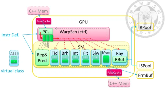
4.2 Warp Scheduling Policy

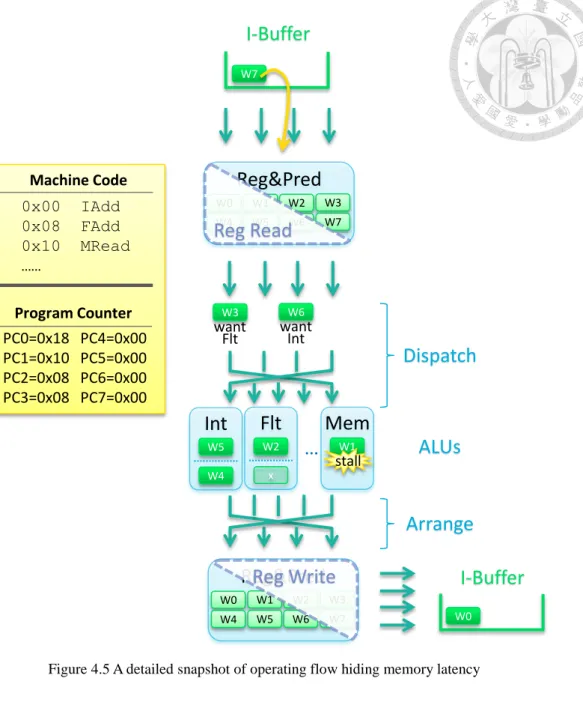
To simplify control unit, our warp scheduling policy is very similar to fine-grain multi- threading. The dispatcher delivers as many warps to ALUs as possible according to their OP-code. For pipelined ALUs, every pipeline stages is filled with different warps.

The arbitration of warps for the same ALU is static priority. By differing the pro- gress, we can avoid warps executing the same instruction and collision at dispatcher.

And it is also simple for implementation.

This policy brings the effect of hiding memory latency. Imagine that the warp with highest priority (w0, for example) initially occupies the computation ALU. Then it might suffer a memory read instruction and still. Meanwhile, the computation ALU is released for low priority warps and so on switching warps. Until the origin warp (w0) finish the memory access, the computation resource is kept without waste.

SM Flt

Int Slw

^Mem

Brh Tid

3 11

1 2

Reg&

Pred

²

ALU

?

virtual class

GPU

WarpSch (ctrl) RPool

ISPool Ray

FrmBuf RBuf

PCs

C++ Mem

Light green: memory unit;

dark green: cycle blocker (pipeline or latency)

Instr Def.

C++ Mem

FakeCache

(28)

Figure 4.5 A detailed snapshot of operating flow hiding memory latency

4.3 Types of ALU

In our configurable multiprocessor, ALUs can be easily plug-in/off and customized. It is not necessarily be a computational ALU and a memory access unit. We also support multiple ALUs having the same type. If there are two integer ALUs, dispatcher can issue two of the warps requiring that kind of ALU in proper way.

It might be a little bit confusing about how to calculate the amount of “cores”.

Here is an idea that imagine an all-purpose ALU, we can easily conclude the amount of cores is equal to such SIMD (single instruction multiple data) ALU width. As for our machine, the different types of ALU can be thought of as the separation of that all-purpose ALU. So the amount of cores in our multiprocessor can be estimated as the maximum of SIMD ALU width across different types of ALU.

Int

W5 W4

Flt

W2 x

…

Mem

W1

stall

W6

wantInt

Dispatch

W3

wantFlt

ALUs

Arrange

W0

I-Buffer Reg&Pred

W0 W1 W2 W3

W4 W5 W6 W7

W7

Reg&Pred

W0 W1 W2 W3

W4 W5 W6 W7

I-Buffer

Reg Read

Reg Write

0x00 IAdd 0x08 FAdd 0x10 MRead

……

PC0=0x18 PC4=0x00 PC1=0x10 PC5=0x00 PC2=0x08 PC6=0x00 PC3=0x08 PC7=0x00

Program Counter Machine Code

(29)

4.3.1 Framework and Typical ALUs

To carry out the feature mentioned above, we define a simple framework for these ALUs. It requires an “ALU type” constant signal, “ALU is free for new task next cycle”

and “warp ID to free” register signal. With such signal, dispatcher can count the amount of resource of each type. After complicated multiplexer executing dispatch policy, customized ALU can receive the decoded instruction with register data (rs, rt), immediate data and OP-code.

In our Ray-Pool based multiprocessor, we define the following ALUs: TidALU (for thread/block indexing and dimension control), BrhALU (for branch control like predicate, jump and function stack), MemALU (for memory access with cache), In- tALU (for integer data computation), FltALU (for floating point data computation), SlwALU (for special function of computation like division and square root), and Ray- ALU (for special function of ray tracing).

In the simulator, we define a virtual class of such ALU. The default operating model is an OP-code dependent fixed latency + constant pipeline stages. The ALUs used in our case are configured as Table 4.1. The notation of “depends” means it over- writes the C++ virtual function for detailed simulation. Those special ALUs are discussed later. The latency and pipeline configurations are illustrated in Figure 4.6.

Table 4.1: Latency and pipeline configuration of ALUs

Types Tid Brh Mem Int Flt Slw Ray

latency

1 1 depends 1 1 1 depends

pipeline

1 2 2 2 3 11 2

(30)

Figure 4.6 Latency and pipeline configuration illustration

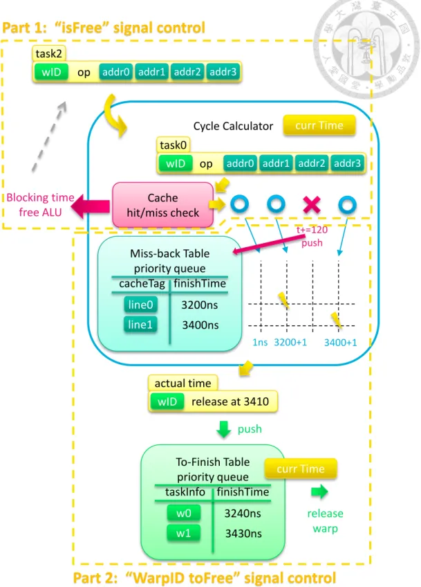
4.3.2 Memory ALU

Both data cache and memory can be mapped to our ALU framework as a new kind of ALU. By dynamically handling the ALU latency, managing “is free” signal and “warp ID to free” signal, we can simulate more complex task like non-blocking cache. The process can be broken into two parts.

latency pipe

task#1 done

isFree

task#1 launch

able to receive new task

3-1=2

3-1=2 4

Configure as L4P3

Configure as L1P4 = fully pipeline with 4 stages

pipe l pipe

1 l

4-1=3

(31)

Figure 4.7 Simulating non-blocking cache

First part is “is free” signal control. Thought we want to simulate a non-blocking cache, there are still some blocking processes. Cache only has limited bandwidth. How- ever, warps contains multiple threads which may request for different cache line. We add a fake 2 way cache that only records the cache tag without storing data, under the consideration of simulation efficiency. Having the cache tag signature is enough for re- porting cache hit or miss. Each cache line access leads to one cycle stall. For coalesced

To-Finish Table priority queue taskInfo finishTime

w0 w1

3240ns

3430ns Miss-back Table

priority queue

cacheTag finishTime

line0 line1

3200ns 3400ns

Cycle Calculator

task0

wID op

addr0 addr1 addr2 addr3

Cache hit/miss check task2

wID op

addr0 addr1 addr2 addr3

t+=120 push

1ns 3200+1 3400+1

actual time

release at 3410 wID

push

curr Time

release warp Blocking time

free ALU

Part 2: “WarpID toFree” signal control

Part 1: “isFree” signal control

(32)

read, the blocking time equals (warp size) / (cache bandwidth) while (warp size) for separate read.

Second part is when to free the warp. It can done by maintaining two timing table.

On one side, we need to take down the time each cache line miss come back. Then, we can calculate the exact time this warp is going to finish. On the other side, we have to keep this finish time in another table since it is still no the time to free that warp. These are implemented by event-based simulation and accelerated by priority queue data structure.

We set a constant cache miss penalty as 120 cycles. The value is chosen from Mi- cron’s DDR3 Verilog model [18]. We try a simple memory controller with close-page policy at the configuration of sg25, JEDEC DDR3-800E, inner clock 400MHz and outer clock 100MHz. It requires about 120 ns to carry 64 bytes data (a cache line).

4.4 Branch Control

Branch control is an import topic as a SIMT processor. We take advantages of predicate registers and PC-RPC stacks, similar to Fung’s work [15].

Simple if-else branches are handled by predicate registers. Each instruction contains a predicate index. That index is mapped to a predicate register recording operation mask for threads in that warp. Data in predicate registers is handled and updated by instructions from BrhALU, only. There are 16 predicate registers for each warp in our implementation.

As for function call or loops, we assign the control over PC-RPC stacks to instructions from BrhALU, too. When calling a function, proper instructions are executed to push a new entry into PC-RPC stacks. The entry is popped at the end of function as PC

>= RPC. Each warp has its own PC-RPC stack.

4.5 Instruction Generating Tool

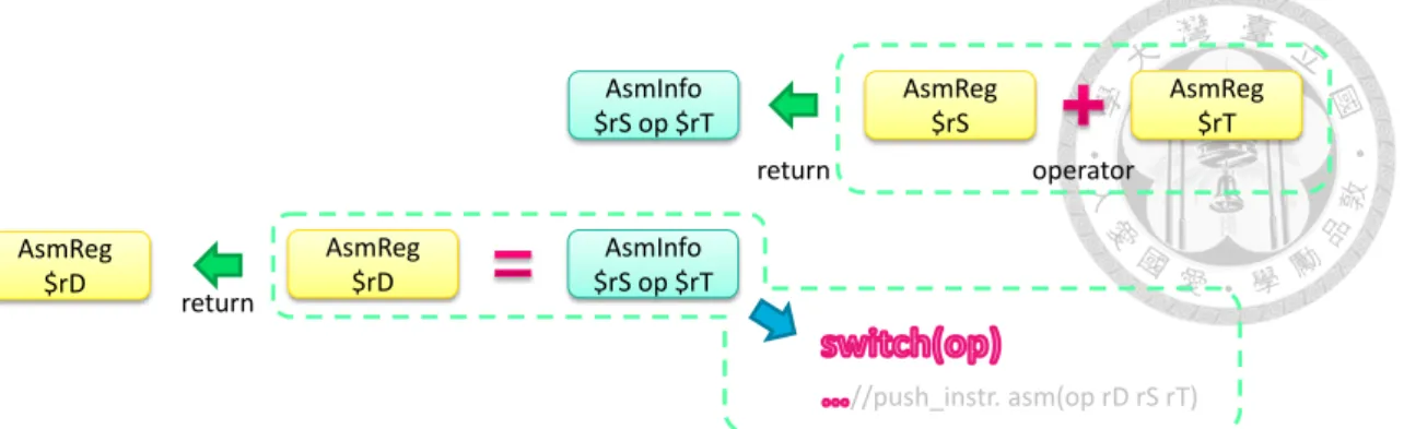
The instructions of different kernels can be generated by our tool in simulator. Since it is difficult to write and maintain machine codes, this tool is helpful in kernel code writing for our self-defined instruction set. This tool is still insufficient as a compiler. It is more like an assembler, but do more things than an assembler.

We make use of operator overloading in C++. We declare a C++ class AsmReg to denote registers. Each AsmReg must come with its register index and a note of its data type (integer or floating point). When two AsmRegs are written to do operations (like addition), we temporarily generate an AsmInfo class. As this AsmInfo meets an assign- ment operator (“=”) with destination AsmReg, our instruction generator would push a proper instruction (iadd rD rS rT, for example) to kernel code storage.

(33)

Figure 4.8 Illustration of instruction generating tool

Meanwhile, these operators used in kernel codes are still primitive C++ operators.

We can easily change the “define” of AsmReg to integer or floating point in primitive C++ while keeping the correct functionality. That is, our generating tool provides two mode: software simulation and hardware simulation.

Pure software simulation is running kernel codes as primitive C++ codes. In this mode, kernel codes are independent of multiprocessor, such as warp scheduler, register, cache and cycles in SystemC simulation. Users can quickly check their algorithm and de-bug in the early phase.

Only the hardware simulation mode make use of SystemC multiprocessor. It is used for verifying simulation details and getting real performance indicator.

Figure 4.9 Two modes of simulation

4.6 Multiple Compute Units

Our multiprocessor simulator support multiple compute units simulation, too. Each compute unit possess a warp scheduler, general and predicate registers, PC-RPC stacks, memory units like instruction and data caches, bus masters to memory and pools and a set of ALUs. Each compute unit is a complete SIMT multiprocessor.

Above from single compute unit, a full system multiprocessor like GPGPUs may has several of these compute units. Due to the hardware constrains, single compute unit cannot grow up unlimitedly. So multiple compute units systems are built for plenty of

AsmReg

$rS

operator

AsmReg

$rT return

AsmInfo

$rS op $rT

return AsmReg

$rD

AsmReg

$rD

AsmInfo

$rS op $rT

//push_instr. asm(op rD rS rT)

dimension setting, prepare memory

kernelPrepare

Both runnable C++ / Asm gen. code

kernelCode

log message, , memory check

kernelEnd

runKernel

#ifdef todoSoftware

for-loop GridDim

#ifdef todoHardware

Asm code finish

install to MP

for all BlkID run warp

scheduler

Ins.txt instrOut

instrIn

(34)

computational requirement. Such system requires a block scheduler, bus and arbiter of bus master in those compute units.

4.7 Optimization for Ray Tracing

To communicate with two pools, keep intersection data and generate ray data it needs some special function units handling such works. We setup the RayALU for doing so.

The local data of intersections and rays is very similar to the role of shared

memory or software defined cache in CUDA [17]. But the system of our ray-pool based ray tracing is data-driven by these intersections and rays. It means that the flow of these driving data must be kept fluently for high efficiency. Here we calculate the efficiency bound by bandwidth to pools:

Bandwidth bound =bandwidth of ray pool, 128 bits per ns

size of ray, 48 bytes = 333𝑀𝑅𝑎𝑦𝑠/𝑠𝑒𝑐 It is very tight for our targeted 100MRays/sec performance. The ray flow must be kept ongoing between pools.

So we design a 3-set local ray memory in our RayALU. One set work as the input buffer for intersection prefetching. Another is used for current computation. While the other act as the output buffer. The roles of these sets swap accordingly by instructions.

Each set of memory contains the full content of rays for total amount of threads in that compute unit. In so doing, we can keep the communication bandwidth with pools near continuing.

Figure 4.10 Local ray memory in RayALU

The local ray memory size is 5.25KB for each set for typical configuration (8 cores with 8 warps). Sum up as about 16KB for each compute units.

However, there are still some limitations to get full utilization of pool bandwidth.

Since the whole multiprocessor is fired up by kernel launching at the same time, rays and intersections are produced and consumed in batches. What’s more, local ray

Set 0

Set 1

Set 2

local R/W export package

Import package

single port

BW: 128 bits (4x4B) nWiB

WarpSize nTiW

Intersection: 21x4B Ray: 12x4B

Current Set Input Buffer Output Buffer

(35)

memory is designed coalesced-wise in order to accelerate local memory read/write by warps. It leads to the batches of packet must be synchronized before and after kernels.

Consequently, though 3-set architecture is seemingly efficient enough, it still requires carefully control both at host about kernel launch algorithm and at kernel codes programming to get practically high efficiency with pools.

Apart from this RayALU, our multiprocessor is still a general-purposed processor like GPGPUs. And it can be viewed as an example of user-defined special ALUs in our configurable multiprocessor.

(36)

Chapter 5 Methodology and Experiment

In this chapter we will discuss about experiments on our simulator. Starts form testing benchmarks, configuration of our simulator and how we measure the performance of proposed system to results and discussion.

5.1 Testing Benchmarks

We test our proposed system on “conference” scene. Such scene has 331K triangles with 36 kind of material and is one of the most popular scenes as ray tracing benchmark. The origin model does not have reflective material. We directly modify all materials with reflective luminous being half of intensity of diffuse luminous. Our testing res- olution is 512x512 pixels with one sample ray per pixel. And there is a single point light as light source.

There are two modes for testing: primary ray only and limited depth of bounce.

The primary ray only case is used for measuring the maximum efficiency of our ray tracer. Each pixel requires an eye ray and a shadow ray for drawing. This case has the highest coherence for memory. As for the other mode, it is closer to real rendering case for ray tracing. Reflective effects can be observe after turning on the bounces. Here we limit the bouncing depth as 5. Both of them are based on the ray tracing algorithm of Whitted-style ray tracing.

(37)

Figure 5.1 Target scene: conference

5.2 Simulation Environment Setup

The followings are configuration and simulation parameters of our simulator.

5.2.1 Two Pools and Traverser

Two pools are configured as the maximum depth of 512 packages. Each ray package is 48 bytes while instruction package is 84 bytes. That is, the ray pool is 24KB in size and intersection pool is 84KB in size. The transfer latency of two pools are both 128 bits per

512x512 px, Whitted-style 36 materials

330K triangles Depth = 1 (Primary)

Depth = 5

conference scene

(38)

nanosecond plus two nanosecond overhead for each request.

The efficiency of Traverser is modeled statically. We use a pure software traverser running the algorithm of AABB BVH tree. We do not varies the delay according to cache or traverse depth since we do not have complete model of hardware traverser. We only assume that it has the equally efficiency with our Shader, transforming 64 rays to intersections as the end of Shader kernel or 1000 nanoseconds when Shader stalls.

The ability of Traverser varies for the experiment of different number of compute units. While doubling the number of compute units in Shader, we also doubles the throughput of Traverser for balancing.

5.2.2 Related Kernel and Host Control Policy

We have three pieces of kernel code: Casting Eye Ray, Casting Secondary Ray and Shading. Casting Eye Ray is the step to generate eye ray by camera and pixel coordi- nates. Casting Secondary Ray is the step to generate reflection ray and shadow ray based on previous intersection. And Shading kernel is the step to draw out light information by non-blocked shadow ray. Being blocked or not is known by null intersection of shadow ray from Traverser.

Figure 5.2 Three kinds of kernel

1 Eye ray

Reflection ray Shadow ray

2

2 3 3

3 kinds of kernel:

① Cast eye ray

② Cast 2

^nd

ray: refl.+shad.

③ Shading by non-blocked shad.

(39)

Kernel codes for two modes (primary ray only and limited depth of bounce) are slightly different. For the mode primary ray only, calculation about reflection in Casting Secondary Ray kernel is skipped. Table 5.1 show the instruction composition of these kernels.

Kernel codes would be slightly different for multiple compute units, too. Because it requires additional codes for control of block dimension especially for Casting Eye Ray kernel. Table 5.1 also show the case of multiple compute units by the right hand side of

“/”. (Left hand side is information of single compute unit.)

Number of instructions (single/multiple compute unit(s)) Kernel Cast Eye R Cast 2^nd R

with refl. R

Cast 2^nd R

without refl. R Shading

N of Instr. 77 / 85 191 110 54 / 55 *

Appr. Time (4w 4c)

636 ns /

671 ns 1138 ns 643 ns 292 ns /

325 ns Composition

for TidALU 2 / 6 1 1 1

for BrhALU 2 / 3 7 5 6

for MemALU 2 4 4 3

for IntALU 33 / 36 54 38 23

for FltALU 24 75 33 10

for SlwALU 1 5 3 1

for RayALU 13 45 26 10 / 11 *

Table 5.1: Number of instructions in different kernel

*: Shading kernel requires additional synchronization to flush local ray memory for multiple compute units.

Kernel Cast Eye R Cast 2^nd R with refl. R

Cast 2^nd R

without refl. R Shading

Consume -- C nIS C nIS C sIS

Produce C nR C nR+CsR C sR --

Notes: C means the number of contents in such kernel; nR means normal ray; sR means shadow ray;

nIS means intersection of normal ray; sIS means intersection of shadow ray.

There are still other mechanism to destroy rays: rays exceeding bouncing depth limit and null intersections are discarded by pools.

Table 5.2: Effect to pools of different kernels

(40)

The kernel launch policy controlled by hosting CPU (or local controller) is showed in Figure 5.3. Be aware that this policy is not the optimal solution, it is just a naive policy. The choice of kernel launch policy involves lots of factor such as intersection pre- load, early launch or wait for high utilization and the latency of control policy to real kernel launch. It can be a new research topic, so is not discussed in our thesis.

Symbols in Figure 5.3 are illustrated here. RP means the number of rays in ray pool and ISP means the number of intersections in intersection pool. As for “sIS” and “nIS”

are different kind of intersections in intersection pool: sIS is intersection of shadow ray while nIS in intersection of normal ray. It is because the Shading kernel and Casting Secondary Ray kernel operate on different kinds of intersections.

Figure 5.3 Kernel choice policy by controller

It is also important to avoid window effect caused by latency of Shader and Tra- verser. Such situation is showed in Figure 5.4. It can be solved by casting eye rays of another tile on the cost of divergence. Overall, it has an efficiency enhancement about 64% (26Mrays -> 41Mrays) under the blockage of 512 contents (not permanently al- lows new tiles for divergence issue) with the configuration of 8 warps, 8 cores and single compute unit. So the later experiments are all based on the policy without window effect.

RP+ISP>0

RP > 48

sIS > 0

Draw out halt

ISP > 8

sIS < nIS

Cast R

_2nd ^{Cast R}^Eye

or halt

Done

Traversal Traversal Traversal Traversal

(41)

Figure 5.4 Window effect avoidance in kernel launch policy

5.3 Performance Indicator

The following performance indicators are used to judge the quality of different configuration of multiprocessor in section 5.4 .

Firstly, the most important indicator is the overall performance for ray tracing.

General performance is measured by dividing the number of rays traced by simulation time. For the case of primary ray only, the number of rays traced is a constant of 512 (width) × 512 (height) × 2 (eye ray and shadow ray) = 512Krays.

As for the measurement of utilization, we have: time utilization rate, resource utilization rate and ALU utilization rate.

Time Util. = 100% × (𝑚𝑢𝑙𝑡𝑖𝑝𝑟𝑜𝑐𝑒𝑠𝑠𝑜𝑟 𝑤𝑜𝑟𝑘 𝑡𝑖𝑚𝑒) (𝑡𝑜𝑡𝑎𝑙 𝑠𝑖𝑚𝑢𝑙𝑎𝑡𝑖𝑜𝑛 𝑡𝑖𝑚𝑒)⁄ Resource Util. = weighted avg. (kernel time, 100% ∙ 𝑡ℎ𝑟𝑒𝑎𝑑𝑠 𝑙𝑎𝑢𝑛𝑐ℎ𝑒𝑑

𝑚𝑎𝑥. 𝑡ℎ𝑟𝑒𝑎𝑑𝑠 𝑙𝑎𝑢𝑛𝑐ℎ𝑎𝑏𝑙𝑒) ALU Util. = 100% − 𝐴𝐿𝑈 𝑎𝑣𝑎𝑖𝑙𝑎𝑏𝑙𝑒 𝑓𝑜𝑟 𝑛𝑒𝑤 𝑡𝑎𝑠𝑘 𝑏𝑢𝑡 𝑛𝑜𝑡 𝑢𝑠𝑒𝑑

𝑚𝑢𝑙𝑡𝑖𝑝𝑟𝑜𝑐𝑒𝑠𝑠𝑜𝑟 𝑤𝑜𝑟𝑘 𝑡𝑖𝑚𝑒

ALU utilization rate is set as subtraction form because ALUs are not consist for tasks.

Some are pipelined, some are fixed latency, and some are mixed while others are complex. ALU utilization rate is measured for each type of ALU separately. It can be a hint about which type of ALU might be the bottleneck of performance.

There is another kind of indicator, the congestion of ALU. We record the average number of waiting task for a busy ALU.

Cast R

_Eye

Traversal

Cast R

_shd may be mixed from diff. tile

Traversal Cast R

_Eye

Traversal another tile

first tile Cast R

_Eye

Traversal

Cast R

_shd

Traversal first tile

Draw out window

effect

window

effect

(42)

ALU Congesion Traffic = 𝐴𝑐𝑐𝑢𝑚𝑢𝑙𝑎𝑡𝑒 𝑞𝑢𝑒𝑢𝑖𝑛𝑔 𝑡𝑎𝑠𝑘𝑠 𝑏𝑜𝑢𝑛𝑑 𝑓𝑜𝑟 𝑡ℎ𝑎𝑡 𝐴𝐿𝑈 𝑚𝑢𝑙𝑡𝑖𝑝𝑟𝑜𝑐𝑒𝑠𝑠𝑜𝑟 𝑤𝑜𝑟𝑘 𝑡𝑖𝑚𝑒

If the congestion traffic is abnormally high, it indicates that it requires more specific resource or architecture improvement for higher performance.

5.4 Experiment of Different Configuration

We measure the performance and related indicators on our proposed system with different configuration. From these experiments, it helps us both in the choice of configuration and the trends when system grows.

5.4.1 Different Warp-Thread Configuration

Tables below show the effect of different configurations on performance and indicators.

Notation of AwBc in Config. rows denote the configuration of A warp(s) and B core(s), which can serves A×B contents in maximum. This content also means the memory re- source required, both in register file and local ray memory. We group up these configuration by number of contents.

Table 5.3: Results of single CU with 16 contents

Results of conference scene (16 contents, single CU)

Config. 1w16c 2w8c 4w4c 8w2c 16w1c

Performance

(Mrays/s) 18.69 19.14 18.69 15.87 10.58

Time Util. (%) 99.52 99.51 100 99.59 99.46

Res. Util. (%) 99.5 99.49 99.35 99.44 78.96

Indicator of different ALUs (Util. : %, Wait : N. of warps)

IntALU Util. 5.82 11.9 23.08 39.35 52.51

FltALU Util. 4.15 8.48 16.45 28.05 37.43

MemALU Util. 18.44 19.46 20.01 18.95 15.13

RayALU Util. 3.9 7.98 15.47 26.38 35.19

IntALU Wait 0 0 0.06 0.71 2.62

FltALU Wait 0 0 0.06 0.37 0.80

MemALU Wait 0 0.47 1.24 2.23 1.60

RayALU Wait 0 0.06 0.26 0.59 0.80

(43)

Utilization of IntALU, FltALU and RayALU increase as numbers of cores de- crease. Fewer resource of computational cores causes higher utilization ratio. MemALU does not follow this rule since the size and bandwidth of data cache keeps the same (8KB, 128Gb/s) throughout different configurations. For RayALU, though the size of local ray memory keeps the same in RayALU, the bandwidth will grow as the configuration of more cores.

(44)

Result of conference scene (32 contents, single CU)

Config. 1w32c 2w16c 4w8c 8w4c 16w2c 32w1c

Performance

(Mrays/s) 31.77 32.85 31.46 29.14 17.78 13.83

Time Util. (%) 99.19 99.16 99.19 99.25 100 99.65

Res. Util. (%) 100.00 100.00 100.00 100.00 65.57 81.05 Indicator of different ALUs

IntALU Util. 4.94 10.22 19.57 36.23 44.2 68.47

FltALU Util. 3.52 7.28 13.95 25.82 31.41 48.80

MemALU Util. 30.82 32.36 31.94 31.32 20.99 19.63

RayALU Util. 3.31 6.85 13.12 24.28 29.55 45.89

IntALU Wait 0 0.01 0.03 0.61 2.03 7.80

FltALU Wait 0 0.01 0.03 0.29 0.76 1.17

MemALU Wait 0 0 0 0 0 0.02

RayALU Wait 0 0.03 0.18 0.44 0.68 1.16

Results of conference scene (64 contents, single CU)

Config. 2w32c 4w16c 8w8c 16w4c 32w2c

Performance

(Mrays/s) 43.76 42.64 40.95 37.31 26.87

Time Util. (%) 86.97 87.85 88.39 99.04 99.31

Res. Util. (%) 94.75 94.50 94.51 87.04 87.80

Indicator of different ALUs (Util. : %, Wait : N. of warps)

IntALU Util. 8.11 15.32 28.9 46.48 67.24

FltALU Util. 5.69 10.83 20.52 33.13 47.79

MemALU Util. 45.02 44.16 43.55 37.64 30.29

RayALU Util. 5.36 10.2 19.3 31.15 44.95

IntALU Wait 0.01 0.03 0.45 2.29 8.28

FltALU Wait 0.01 0.04 0.18 1.03 1.32

MemALU Wait 0.66 1.6 3.26 4.69 4.71

RayALU Wait 0.01 0.11 0.34 0.67 1.37

Figure 5.5 below compares the relationship between performance and different

(45)

configurations.

Figure 5.5 Performance of different configurations (single CU)

Figure 5.6 Normalized Performance of different configurations (single CU)

4.0 8.0 16.0 32.0 64.0 128.0

32 16 8 4 2 1

Performance log2 (Mrays/s)

Number of cores

Different Configuration (single CU)

64contents 32contents 16contents

0.5 1.0 2.0 4.0 8.0 16.0 32.0

32 16 8 4 2 1

Perf. per core log2 (Mrays/s)

適用於光池加速光線追蹤繪圖之多核心處理器硬體架構設計

國立臺灣大學電機資訊學院電子工程學研究所 碩士論文

Graduate Institute of Electrics Engineering

College of Electrical Engineering and Computer Science National Taiwan University

Master Thesis

適用於光池加速光線追蹤繪圖之 多核心處理器硬體架構設計

Ray-Pool Based Configurable Multiprocessor Design for Ray Tracing

謝明倫 Ming-Lun Hsieh

指導教授：簡韶逸 博士 Advisor: Shao-Yi Chien, Ph.D.

中華民國 104 年 9 月

September 2015

誌謝

摘要

Abstract

Contents

List of Figures

List of Tables

Chapter 1 Introduction

1.1 Physically-Based Rendering

1.1.1 Rendering Equation

1.1.2 Whitted Style Ray Tracing

1

Eye ray

Reflection ray Shadow ray

2

4

3 5

① Cast eye (primary) ray

② Cast 2

ray: reflection ray + shadow ray

③ Shading by shadow ray generated in ②

④ Cast 2

ray form reflection ray

⑤ Shading by shadow ray generated in ④

1.2 Limitations of Current GPUs for Ray Tracing

1.3 Motivation and Target

Rasterization-based

• Traditional method

Ray tracing-based

• Light transport simulation

Types Basic rendering

(Primary rays)

Typical effects (Traverse at depth of 5)

480p, 30fps

480p, 60fps

720p, 30fps

720p, 60fps

1.4 Thesis Organization

Chapter 2

Previous Work

2.1 Ray Core

2.2 SGRT

2.3 PowerVR GR6500

2.4 Short Summary

GTX680 [9]

Optix [10] RayCore SGRT PowerVR

GR6500 Ours

Year

Process

Type

Clock

N Cores

GFLOPS

BW(GB/s)

Area

Mrays/s

(Primary)

Chapter 3

System Overview

3.1 Main Concept

3.2 System Architecture

Shader Traverser

Ray Pool

Intersection Pool Image Film

Ray Ray

SIMT Multi-

processor HW ASIC

Target Chip

DRAM instr.

const triangle material

國立臺灣大學電機資訊學院電子工程學研究所碩士論文

適用於光池加速光線追蹤繪圖之多核心處理器硬體架構設計

指導教授：簡韶逸博士 Advisor: Shao-Yi Chien, Ph.D.