基於深度學習方法之相機定位

(1)

國立臺灣大學電機資訊學院資訊網路與多媒體研究所碩士論文

Graduate Institute of Networking and Multimedia College of Electrical Engineering and Computer Science

National Taiwan University Master Thesis

基於深度學習方法之相機定位

Camera Re-Localization with Deep Learning Methods

蔡侑霖 Yu-Lin Tsai

指導教授：洪一平博士 Advisor: Yi-Ping Hung, Ph.D.

中華民國 109 年 7 月 July, 2020

(2)

(3)

誌謝

碩班兩年時光荏苒，不知不覺即將到了這趟探索旅程的終點。首先最感謝我的指導教授洪一平老師，老師一路以來對於研究以及表達的嚴謹要求，不斷激勵我們進步，同時提供了相當完善的實驗環境和設備，讓我們在研究及追求真理時少繞了許多遠路。感謝陳祝嵩教授，老師額外主持的讀書會，提供我們能一個能彼此激盪的機會，每次的會議老師也無私的提供自己專業領域的見解，讓我無論在論文的研讀或研究上都有所精進。感謝同屆一起奮鬥的大家，俊賢、禹達、曜至、大中、琬庭、曜福，感謝你們為實驗室付出了這麼多，也感謝這兩年間互相扶持、討論，我受到你們的幫助遠遠多出我所付出，真的非常感謝。感謝學長姐們，一路上給我的指點，無論是在學業上或是人生歷練上的，都讓我獲益良多。感謝學弟，冠維和濬榕兄，在研究上的討論給了我很多幫助，茶餘飯後的閒聊也是我在實驗室難忘的時光之一。感謝台大羽球隊，給了我一個與眾不同的大學生活，磨練我的身心，讓我不再畏懼困難的挑戰。感謝我的家人，總是在背後默默支持著我，相信我的決定，

讓我有自信及餘裕好好料理人生。感謝我的女朋友陳郁，妳的陪伴、鼓勵以及督促，

緊密的和我求學生涯編織在一起，使其多采多姿並值得回味。謝謝每個曾經幫助過

我的人，是你們使我成為更好的人，衷心地感謝大家。

(4)

中文摘要

基於影像的定位是希望透過影像資訊推測相機自我位置的問題，同時，對於自駕車、擴增實境、智慧機器人來說是一個關鍵且基礎的技術。近年來，隨著算力的提升和深度學習的發展，許多研究嘗試利用卷積網路強大的特徵描述能力來幫助相機自我定位。然而，當使用場域改變時，這些方法都必須花很多力氣和時間重新訓練其模型，同時顯示其泛化能力相當受到限制。基於圖像搜索概念的定位架構提升了在不同場景的泛化能力，但在預測相機相對位置時而會受限於場景。我們基於圖像檢索的概念提出了一個相機定位的架構，在計算相機相對位置時討論了更多傳統的空間幾何。同時，我們也嘗試用深度學習的方法預測影像深度資訊並加強了我們方法的定位精準度。實驗結果顯示我們的方法和現在最先進的方法有並駕齊驅的定位能力，此外，利用模型壓縮讓我們的定位流程能達到幾乎即時運行。因此，

我們認為融合傳統相機方法和深度學習是一個相當有潛力的發展方向。

關鍵字：基於影像的定位、相機定位、深度學習、擴增實境

(5)

ABSTRACT

Image-based localization is used to estimate the camera poses within a specific scene coordinate, which is a fundamental technology towards augmented reality, autonomous driving, or mobile robotics. As the advancement of deep learning, end-to-end approaches based on convolutional neural networks have been well developed. However, these methods suffer from the overhead of reconstructing models while been applied to unseen scene. Therefore, image retrieval-based localization approaches have been proposed with generalization capability. In this paper, we follow the concept of image retrieval-based methods and adopt traditional geometry calculation while performing relative pose estimation. We also use the depth information predicted from deep learning methods to enhance the localization performance. The experimental result in indoor dataset shows the state-of-the-art accuracy. Furthermore, by distilling and sharing the encoder of global and local feature, we make our system possible for real-time application. Our method shows great potential to leverage traditional geometric knowledge and deep learning methods.

Keywords: Image-based localization, Camera pose estimation, Deep learning, Augmented Reality.

(6)

LIST OF FIGURES

Fig. 1-1 Visualization of our localization procedure ... 3

Fig. 3-1 Our localization pipeline. ... 9

Fig. 3-2 Image retrieval pipeline example using NetVLAD ... 10

Fig. 3-3 Four cases of R/t ... 12

Fig. 3-4 Pose filtering with RANSAC. ... 13

Fig. 3-5 Case illustration with four non-intersecting lines ... 16

Fig. 3-6 Depth estimation training and inference procedure ... 18

Fig. 3-7 Multi-task distillation framework ... 20

Fig. 4-1 Sample image from the 7-Scenes dataset ... 21

(9)

LIST OF TABLES

Table 4-1 Result on 7 Scenes dataset of comparing different feature methods ... 23 Table 4-2 Result on 7 Scenes dataset of comparing state-of-the-art methods ... 24 Table 4-3 Result on 7 Scenes dataset with depth information ... 25 Table 4-4 Result on 7 Scenes dataset of comparing methods using 3D information ... 25 Table 4-5 Computation cost [ms] for each step ... 26 Table 4-6 Generalization performance ... 28

(10)

Chapter 1 Introduction

Camera localization, or image-based localization is a basic problem in robotics and computer vision. It refers to the process of solving the precise 6 Degree-of-Freedom (DoF) camera pose of a query image according to known reference like pre-built 3D point cloud model coordinate. This key technology is widely used in computer vision applications, including autonomous driving in GPS-denied environment, virtual reality, and device with augmented reality features like mobile phones and head mounted display (HMD) like HoloLens. More broadly, visual localization is also an important component of computer vision tasks like Structure-from-Motion (SfM) and the mapping part of Simultaneously Localization and Mapping (SLAM).

There are three generally kinds of the imaged-based localization approaches, namely structure-based camera localization, absolute pose regression camera localization, and image retrieval-based camera localization. The structure-based camera localization refers to the approaches which estimates the 6 DoF pose with the correspondence between local feature from query image and pre-built SfM point cloud model. The correspondence between 2D and 3D usually is established under the reliable and repeatable feature descriptor. However, these structure-based methods rely on a point cloud with superior quality and suffer from time consuming feature extractor procedure like SIFT [1].

In recent years, as the huge impact of many computer vision task benefit from the extraordinary dense feature extraction ability of convolutional neural network (CNN), many researches tried to employ deep learning architecture in predicting camera pose.

Absolute camera pose regression proposes an end-to-end deep learning method, like

(11)

Rather than traditional mathematical geometry procedure, these approaches tried to simulate the optimization process through the composition of convolution layers. In spite of the high-speed due to their end-to-end structure, it mostly requires lots of effort and time to fine-tune while changing the scene.

To conquer the limitation of generalization, image retrieval-based camera localization methods like NNet [3] leverage the success of image classification, semantic segmentation, and image retrieval. Instead of direct predict camera pose, these methods attempt to regress the relative pose between query image and most similar images selected by image retrieval. Although image retrieval-based camera localization methods hold better generalization performance, the procedure of relative poses estimation by regression is still hard to extend to another scene.

In this work, we propose an image retrieval-based camera localization pipeline with pairwise relative pose estimation using both traditional geometry methods and deep learning methods shown in Fig. 3-1. The usage of essential matrices prevents the disadvantage of the needing of scene-dependence hyperparameters and improves the ability of generalization. With the improvement of depth estimation using deep learning, our framework also contains the 2D-3D scenario using the depth map inferenced from database RGB images and their ground truth camera pose. Inspired by HF-Net [4], we try to speed up the whole localization process by distilling both encoders of local and image representation feature and sharing one encoder. With the flexibility of our method, we compare the deep learning method to traditional method in each component of localization pipeline and thus recommend the best combination from these methods with respect to robustness and efficiency.

(12)

Our contributions are as follows. First, we establish a flexible image retrieval-based camera pose localization pipeline without a 3D point cloud model. Each component can be easily replaced with other suitable method. The second contribution is that our framework holds a capability to generalize in every unseen scene by adopting traditional geometry process in relative pose estimation step. Last but not least, our localization result using only 2D information competes with the state-of-the-art image-based localization methods, while our results under 2D-3D case outperform the above approaches. Yet, our results using estimated depth mildly inferior to structure-based localization methods.

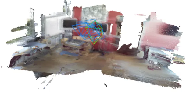
Fig. 1-1 Visualization of our localization procedure. The green one denotes the ground truth pose of query image, the blue ones denote the candidate image pose obtained by

image retrieval, and the red one is the result pose estimated by our approach.

(13)

Chapter 2 Related Work

In this section we review the previous works that relate to components of our method, namely: 6-DoF Visual Localization, Local Features and Feature Matching, and Depth Estimation.

2.1 6-DoF Visual Localization

2.1.1 Structure-based Localization

Structure-based localization methods perform direct 2D-3D matching between 2D pixel position of query image and 3D points in a 3D structure-from-motion model. The 2D-3D correspondences are used to estimate the camera pose of the query image by applying an n-point- pose solver such as [5, 6] within a RANSAC loop [7] .

Rather than obtaining the 2D-3D correspondences from descriptor matching, some previous works tried to predict the 3D position of each pixel by 3D scene coordinate regression using convolutional neural networks [8-11] or random forest [12, 13]. 3D coordinate regression methods currently achieve a higher pose accuracy at small scale, but have not yet been shown to scale to larger scene.

Furthermore, HF-Net [4] provides a camera localization pipeline using efficient deep learning global and local feature. Besides the ability to handle large scale scenes, HF-Net [4] shows an outstanding robustness in particularly challenging conditions.

2.1.2 Image Retrieval Localization

Image retrieval methods can only provide an approximate pose of the most similar

(14)

image form database to the query image. However, the retrieval result is not precise enough due to the discretization of database. The image retrieval localization often contains the relative pose estimation phase to predict the query image pose from one or multiple similar database images.

For traditional image retrieval part, VLAD [14] proposed a representation vector of aggregated local feature based on BoF (Bag-of-Features) and fisher vector concepts.

After calculating each database local features, BoF would perform feature center clustering like k-means clustering [15]. The distribution of local features in image is the representation vector. Meanwhile, fisher vector utilizes the means and covariance of GMM (Gaussian Mixture Model) to represent each image.

In recent years, many researches tried to enhance the description ability by deep learning technique. The NetVLAD [16] is presented to learn both the descriptor and feature center by CNN and the carefully-designed networks.

Back to localization issue, as mentioned above, image retrieval can only provide approximate poses. More precise poses can be obtained by pairwise relative pose estimation. NNnet [3] learned the relative pose between RGB image pairs and proposed a images localization pipeline contained image retrieval and robust pose estimation.

Moreover, RelocNet [17] proposed a network is jointly trained for the tasks of image retrieval (based on a novel frustum overlap distance) and relative camera pose regression.

Yet, [18] stated that, while being among the best-performing end-to-end localization approaches, current direct relative pose regression techniques do not consistently outperform an image retrieval baseline.

(15)

2.1.3 Absolute Camera Pose Regression

Absolute camera pose regression aims to regress the camera pose and orientation through the trained deep neural network models.

PoseNet [2] tried to learn complete camera localization pipeline through a single CNN model. As the first work trying to leverage the power of feature extraction in CNN, PoseNet [2] has been extended in many ways. PoseLSTM [19] proposed a novel architecture combined CNN and LSTM [20] for camera pose estimation. MapNet [21]

presented a DNN with a new parameterization for camera rotation, the logarithm of unit quaternion

VLocNet [22] proposed the architecture consisting of a global pose regression sub- network and a Siamese-type relative pose estimation sub-network, taking two consecutive monocular images as input and jointly regresses the 6-DoF global pose. Furthermore, VLocNet++ [23] is a novel framework for jointly learning semantics, visual localization and odometry from consecutive monocular images.

2.2 Local Features

As mentioned above, structure-based localization employed hand-crafted feature detectors and descriptors. The FAST [24] corner detector was the first architecture to perform high-speed interest point detection. The ORB [25] proposed a very fast binary descriptor based on BRIEF [26] and was adopted in ORB-SLAM [27] as an efficient and robust component toward real-world and real-time scenario. The Scale-Invariant Feature Transform, or SIFT [1], is still the most well-known traditional feature detector and descriptor when it comes to camera localization or structure-from-motion issues in

(16)

computer vision.

Learned local features are recently been developed to replace the hand-crafted features. Dense pixel-wise features are spontaneously generated by CNN and are intuitively utilized for feature matching and camera localization [10, 28]. However, the dense matching between dense features are time consuming. Sparse learned features architecture regresses sparse interest points and their descriptors from single encoder, such as LIFT [29] and SuperPoint [30]. These end-to-end procedures are fast to predict and have also been shown to outperform the traditional methods.

2.3 Depth Estimation

In classic computer vision, the depth of image is usually computed from a given set of images, such as image pair from stereo camera. In deep learning based computer vision, researchers put more effort on predicting the depth map from monocular image and treat this kind of problem as an image to depth regression issue. Learning depth from single image consist of two forms. The supervised approach tries to regress the result depth map as the given ground truth depth map, while the self-supervised focuses on predicting the depth map under the traditional geometry constraints.

End-to-end supervised learning [31, 32] have been explored to show their good performance than traditional methods. Fully supervised approaches require precise ground truth depth map while training the model. However, this is a challenge to acquire in varied real-world setting.

In the absence of ground truth, one of the alternative approaches is self-supervised

(17)

image reconstruction information as supervisory signals. Zhou et al. [33] proposed a jointly self-supervised learning framework, SfMlearner, which predicts depth map and 6- DoF pose simultaneously from monocular frame sequence. However, the strong geometry constraint used in SfMlearner is that the scene must be in a static environment. Therefore, Zou et al. [34] further added an optical flow estimation to distinguish rigid and non-rigid components.

When it comes to depth reconstruction, the monocular-based approach uses images sequence from single camera as source data would suffer from scale inconsistency problem. Bian et al. [35] proposed a geometry consistency loss between nearby frame to fix the scale of inferenced depth maps.

(18)

Chapter 3 Method

3.1 Pipeline

The scalable pipeline takes a RGB query images as input and results a 6 degrees of freedom camera pose within database scene. Our approach roughly follows the architecture of image retrieval localization pipeline. Rather than direct regressing the relative pose between image pairs like [3, 17], we introduce the classic relative pose estimation method based on essential matrix. For the dataset with depth information, we can direct inference the absolute camera poses through P-n-P algorithm.

Our pipeline consists of three modules: (1) Image Retrieval (2) Feature Extraction and Feature Matching (3) Relative Pose Estimation.

Notably, we can easily use either traditional or learning-based methods in each part of our pipeline. In Chapter 4, we compare the robustness and efficiency of different kind of approaches.

(19)

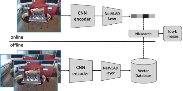
3.2 Image Retrieval

In order to find the most similar database image to query image, it is important to convert both the database and query images into suitable representation vector. We perform image retrieval by DenseVLAD descriptor [36] and NetVLAD descriptor [16], which has been shown to work under challenging conditions [37]. Compared to other learned pipelines for image retrieval [38, 39], NetVLAD [16] and DenseVLAD [36] show better generalization to unseen scenes, which fit well to our pipeline.

As shown in Fig. 3-2, the pipeline contains online and offline parts. In the offline part, we first calculate all the representation vectors of database images and store them as vector database. In the online querying part, after extracting global image descriptor, we compare the query descriptor d_" to the pre-computed descriptors d_# by nearest neighbor search. In practical, we express the similarity of two vector by cosine similarity and use K-D tree as indexing structure.

Fig. 3-2 Image retrieval pipeline example using NetVLAD

(20)

3.3 Feature Extraction and Matching

Local feature extraction

To estimate the relative pose of retrieved pairs, we need to find the correspondence between images. InLoc [10] performed dense matching of CNN encoded feature map while estimating the relative pose. NNet [3] tried to directly regress the relative pose through Siamese neural network with two representation branches connected to a common regression part.

However, matching dense features is intractable with limited computing power, and both of these approaches are struggling with generalizing to other scenes. In [40] shows that directly using data-driven approaches for pose estimation yields less accurate results.

Therefore, we aim on sparse feature detectors which can easily be sampled from dense features and fast to predict.

In this work, we compare three sparse feature extractors, SIFT [1] , ORB [25] , and SuperPoint [30]. SIFT is still the most well-known traditional feature detector and descriptor and serves as the best traditional hand-crafted feature benchmark. Although SIFT has really great performance of accuracy, most real-time application like SLAM won’t adopt SIFT due to the time consuming processing time. Take efficiency into consideration, we decide to choose ORB as one of the feature extractor candidate. As for learning-based method, SuperPoint learns from self-supervision and performs sparse interest point detection.

Feature Matching

Finding good correspondence between features extracted from image pair also has

(21)

use brute force searching to find the most similar local feature. The similarity of two features is described as inner product. To make the procedure more robust and ensure the quality of correspondence, we adopt the ratio test proposed by [1] using threshold 0.8.

Meanwhile, we speed up the matching process using PyTorch if there is GPU available.

3.4 Relative Pose Estimation

As shown in Fig. 3-1, our framework contains two cases, 2D-2D and 2D-3D case, and the difference comes from using depth information or not. In this section, we introduce these cases step by step.

3.4.1 2D-2D case

With correspondence computed from Section 3.3., we can estimate the essential matrix by five-point [41] method in RANSAC [7] loop. Essential matrix can be decomposed into four relative poses, as shown in Fig. 3-3., R, t , R, −t , R⁽, t , (R⁽, −t).

Next, we can verify the correct combination by examining the depth is positive or not based on matched feature points.

Fig. 3-3 Four cases of R/t

Since we cannot determine the correct scale of t, the absolute poses cannot directly

(22)

candidate image. Hence, we reformulate the problem to pose hypothesis filtering with RANSAC loop. This process is illustrated in Fig. 3-4.

Fig. 3-4 Pose filtering with RANSAC.

The relative pose estimated from 2D-2D matched features can be expressed as a line. R_,- and t_,- denote the rotation and translation matrix of training image. R_-. and t_-. denote the rotation and translation matrix of relative pose estimated from pipeline, and 𝜶 denote the unknown scale. We express the estimated pose of query image multiplied by relative pose as shown in Equation (3-1).

𝑅₁₂ 𝜶𝑡₁₂

0 1 𝑅₆₁ 𝑡₆₁

0 1 = 𝑅¹²𝑅₆₁ 𝑅₁₂𝑡₆₁+ 𝜶𝑡₁₂

0 1 (3-1)

The absolute camera pose 𝑐 can be described as Equation (3-2) with its camera

projection matrix 𝑅 and 𝑡 . Therefore, with the parameters in Equation (3-1), the estimation line is written as Equation (3-3).

𝑐 = −𝑅^:𝑡 (3-2)

(23)

𝑒𝑠𝑡𝑖𝑚𝑎𝑡𝑖𝑜𝑛 𝑙𝑖𝑛𝑒 = −𝑅₆₁^:𝑅₁₂^: 𝑅₁₂𝑡₆₁− 𝜶𝑅₆₁^:𝑅₁₂^: 𝑡₁₂ (3-3)

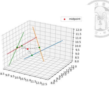
In RANSAC loop, we random select two pairs from Top-K retrieved pairs. The hypothesis pose is the closest point to the two selected estimation line. We can easily obtain the point from the midpoint of the common perpendicular line. P_D and P_E are the point in the estimation line, while v_D and v_E are the vector of the lines respectively.

𝑃_D+ 𝑡𝑣_D + 𝑢 𝑣_D×𝑣_E = 𝑃_E + 𝑠𝑣_E (3-4)

ℎ𝑦𝑝𝑜𝑡ℎ𝑒𝑠𝑖𝑠 𝑝𝑜𝑠𝑒 = ^N^O^P6Q^O^PN_E ^R^PSQ^R (3-5)

The orientation of hypothesis is obtained by the spherical linear interpolation

(SLERP) of two quaternions. q_U and q_V are the quaternions of estimated pose from hypothesis pair and ⊗ denotes SLERP operation.

𝑞 = 𝑞_Y ⊗ 𝑞_V (3-6)

To evaluate a hypothesis, we find the distance between hypothesis pose and each estimation line. If the distance is under the threshold, that estimation line would be considered as one of the inlier line set. P_. and v_. is the point and vector of estimation line and P_Z is a point in 3D coordinate from hypothesis pose.

𝑒𝑟𝑟𝑜𝑟 𝑑𝑖𝑠𝑡𝑎𝑛𝑐𝑒 = ^N^]^N_Q^{^}^×Q^]

] (3-7)

After hypothesis pose passes the inlier test, the final hypothesis should be refined by all the inlier line. The problem is transformed into finding the closest point to multiple estimation lines. We first formulate single line:

(24)

_`__a

b_a =^c`c_d ^a

a =êè_f â

a = 𝑡_Y,

1 0 0 −𝑎_Y 0 1 0 −𝑏_Y 0 0 1 −𝑐_Y

𝑋 𝑌 𝑍 𝑡_Y

= 𝑥_Y 𝑦_Y

𝑧_Y (3-8)

Then we can obtain the equation of multiple lines assuming that the hypothesis pose lies on the intersection of lines perfectly.

𝐴𝑥 = 𝑏 (3-9)

1 0 0 −𝑎_D 0 … 0

0 1 0 −𝑏_D 0 … 0

0 0 1 −𝑐_D 0 … 0

1 0 0 0 −𝑎_E … 0

0 1 0 0 −𝑏_E … 0

0 0 1 0 −𝑐_E … 0

… … … 0

1 0 0 0 0 … −𝑎_o

0 1 0 0 0 … −𝑏_o

0 0 1 0 0 … −𝑐_o

𝑋 𝑌 𝑍 𝑡_D 𝑡_E

… 𝑡_o

= 𝑥_D 𝑦_D 𝑧_D

… 𝑥_o 𝑦_o 𝑧_o

(3-10)

For the general solution, we ignore the least-squares technique as it is not able to provide solutions once A is rank-deficient. By using SVD, we derive the general solutions of the nearest approach for all cases of multiple lines in 3D space.

𝑥 = 𝐴^P∗ 𝑏 (3-11)

In our approaches, we will examine the number of inlier of 𝑥 to ensure the quality of final hypothesis.

(25)

Fig. 3-5 Illustration of closet point to four non-intersecting lines in 3D space As for orientation part of multiple inliers, we intuitively calculate the average of all quaternion vector by SLERP.

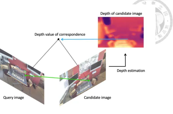
3.4.2 2D-3D case

The 2D pixel can be inverse projected into 3D coordinate with known camera intrinsic, camera pose within specific scene, and depth information. After finding correspondence described in Section 3.3, we can solve the localization problem using PnP algorithm since the matched pixels in candidate image are interpreted as 3D points in scene as shown in Fig. 3-6. In RANSAC loop, we adopt P3P to generate the pose hypothesis and set the minimum number inlier threshold as 12. Next, we optimize the pose hypothesis by minimizing the projection error of all inliers points. In this part we simply use the opencv library solvePnPRansac and solvePNP.

(26)

Fig. 3-6 Illustration of 2D-3D case

3.5 Depth Estimation

Review our proposed framework, we would need a dense depth map of candidate RGB images when performing 2D-3D pose estimation. Even though some datasets have collected depth information already like 7-Scenes dataset, in this work we want to calculate all the information from solely RGB information.

3.5.1 Depth Estimation Framework

Inspired by self-supervised learning framework of Zhou et al. [33], we modify the origin framework to reconstruct 3D scene depth from continuous image sequence. Since we have the ground truth of each training image pose, the framework would be able to take precise 6-DoF information as one of the supervisory signal to reconstruction. In other words, our procedure doesn’t need to predict the pose of each training image and we aim on training the network predicting the depth information.

(27)

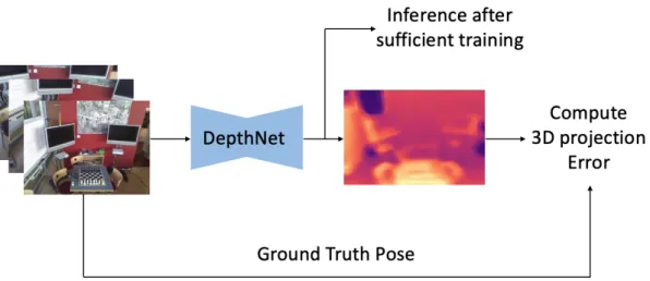
The depth estimation framework consists of a neural network, DepthNet, taking RGB frames as input and predicting depth map as output shown in Fig. 3-7. Let D_, denote predicted depth of target view, and T_,→‹ denote the relative pose calculated from ground truth pose T_‹ and T_,. With known camera intrinsic K, we can project p_,, the homogeneous coordinate of a pixel from target view, onto source view p_‹ by

𝑝_S~𝐾𝑇_6→S𝐷₆ 𝑝₆ 𝐾^`D𝑝₆ (3-12)

At this point, the 3D projection error can be computed by the difference between the source view projected from target view and the original source view. After sufficient training epochs, the tuned DepthNet is able to inference more steady and optimized depth result.

Fig. 3-7 Depth estimation training and inference procedure

3.5.2 Loss Term

In this section, we will present each component of our loss, including appearance matching loss and geometric loss. Our overall objective function can be formulated as follows:

(28)

ℒ = 𝛼ℒ_b“+ 𝛽ℒ_• (3-13)

where ℒ_–— stands for proposed appearance matching loss and ℒ_˜ stands for geometric loss.

Appearance Matching Loss

The key supervisory signal for our depth estimation is calculated from view synthesis. During the training, we project the source view image I_Uš^‹ to target view image I_Uš^, by inverse warping with estimated D_‹ and ground truth relative pose T_‹→,. The appearance matching loss is described by the appearance difference between target view image I_Uš^, and synthesized image I_›œ^,. Follow the work [42], we use the combination of two terms, L1 distance and single scale SSIM [43], describing the photometric difference as ℒ_–—^, :

ℒ_b“⁶ = ^D_• 𝛼^{D`žžŸ Ÿ}^a¡

¢,Ÿ_£¤^¢

E + 1 − 𝛼 𝐼_YV⁶ − 𝐼_¦§⁶ _D

Y,V ∈• (3-14)

Here, V denotes the points that successfully project from the source view to the target view, while successful projection means that the result pixel coordinate falls in the target image. V means the number of the successful points. We use the simplified SSIM with a 3×3 block filter and set α to 0.5 as a fixed weight.

Geometric Loss

To enforce the geometry consistency on predicted result, we aim on minimize the difference between the depth values of correspondence pixel from different view. With the relative pose T_,→‹ computed from ground truth pose, we can project the predicted

(29)

[35] and simply define the geometric loss as:

ℒ_˜ 𝑡, 𝑠 = _•^D ^¬_¬^¢→- ^{“ `¬}^-^® ^“

¢→- “ P¬_-^® “

“∈• (3-15)

where D_‹⁽ is the interpolated depth map from the estimated map D_‹. The difference obtained from each input frame is normalized by the sum of two depth map.

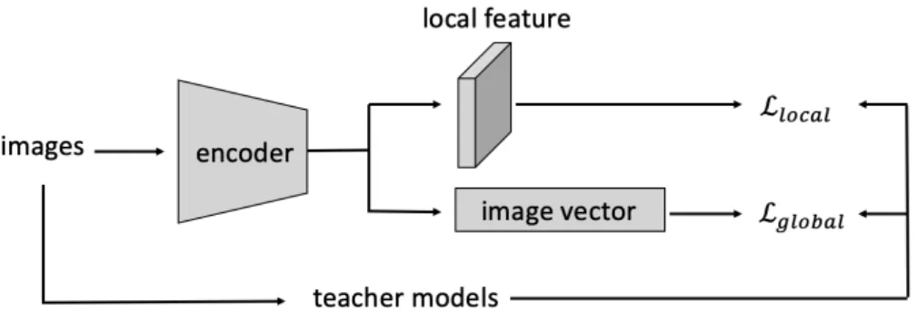
3.6 Model Distillation

In the relative pose estimation pipeline, we need to perform feature extraction twice for the purpose of image retrieval and local feature matching. Consider the state-of-the- art image retrieval approach, we can find that the representation vector is usually composed of local features. Therefore, it is a natural idea to predict both representation vector and the local feature map of images from shared weighted encoder.

In the work [44] , NetVLAD is distilled into MobileNetVLAD based on MobileNet backbone in order to enhance the efficiency. In [4], HF-Net furtherly distills both encoder from NetVLAD and SuperPoint with MobileNet. In this work, we basically follow the concept of HF-Net. We also use teacher student learning architecture to train a shared light weight model.

Fig. 3-8 Multi-task distillation framework

(30)

Chapter 4 Experiments

4.1 Dataset

Indoor Dataset

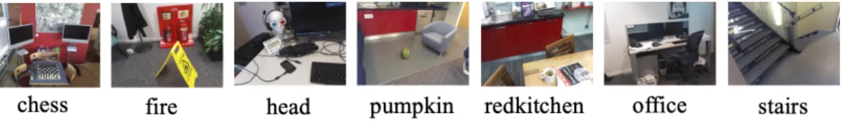
The 7-Scenes dataset, provide by Microsoft, is recorded in indoor environment with tracked RGB-D camera. The dataset consists of seven different indoor scenes and all frames are collected with handheld Kinect RGB-D camera at 640*480 resolution. The ground truth pose of each frame and the dense 3D model are computed by KinectFusion[45]. The 7-Scenes dataset covers an area of 12 square meters and the seven scenes are namely, chess, fire, heads, office, pumpkin, red kitchen, stairs. The sequences are split into training and testing part, which contains 26000 images for training and 17000 images for testing.

Fig. 4-1 Sample image from the 7-Scenes dataset

4.2 Localization Result

The localization result parts focus on the accuracy of pose estimation. We show the experimental results according the procedure of our framework, image retrieval, localization result with relative pose estimation under 2D-2D case and 2D-3D using depth information. Note that the following result tables present the median localization error of position [m] and orientation [deg].

(31)

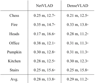
4.2.1 Image Retrieval

The localization result of these image retrieval methods comes from the accuracy of the pose of most similar image retrieved from database. To compare the accuracy of image retrieval methods, we evaluate the pose of the most similar image. As shown in Table 4-1, we can tell that NetVLAD [16] and DenseVLAD [36] hold nearly the same performance. However, due to high computation cost of DenseVLAD, we adopt NetVLAD as our image retrieval method in the following experiment.

NetVLAD DenseVLAD

Chess 0.25 m, 12.7◦ 0.21 m, 12.5◦

Fire 0.35 m, 14.7◦ 0.33 m, 13.8◦

Heads 0.17 m, 16.6◦ 0.28 m, 11.2◦

Office 0.38 m, 12.1◦ 0.31 m, 11.3◦

Pumpkin 0.30 m, 12.8◦ 0.31 m, 11.3◦

Kitchen 0.28 m, 12.5◦ 0.30 m, 12.3◦

Stairs 0.25 m, 15.6◦ 0.25 m, 15.8◦

Avg. 0.28 m, 13.8◦ 0.29 m, 11.2◦

Table 4-1 Result on 7 Scenes dataset of comparing different image retrieval methods

4.2.2 2D-2D case

Comparison of different feature extraction methods

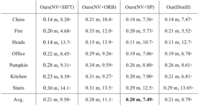
We first make an evaluation of our localization framework with several chosen feature extractors under 2D-2D case. NV denotes that we apply NetVLAD [16] as our image representation vector extractor. For local feature methods, SIFT [1] is still considered as one of the most robust feature detector and descriptor. However, the cost of

(32)

computation time should also be taken into account due to the efficiency issue of localization applications. Therefore, we treat ORB [25] as a more fast and practical local feature extractor. Meanwhile, SP denotes SuperPoint [30] which represents one the deep learning method predicting sparse keypoints and their descriptors. Distill means the feature extractor architecture we introduce in 3.6 using the same encoder in both global and local feature descriptor phase.

Ours(NV+SIFT) Ours(NV+ORB) Ours(NV+SP) Our(Distill) Chess 0.14 m, 8.20◦ 0.21 m, 10.4◦ 0.14 m, 7.56◦ 0.14 m, 7.47◦

Fire 0.20 m, 4.68◦ 0.33 m, 12.0◦ 0.20 m, 5.73◦ 0.21 m, 5.52◦

Heads 0.14 m, 13.7◦ 0.15 m, 13.9◦ 0.11 m, 10.7◦ 0.11 m, 12.7◦

Office 0.22 m, 8.45◦ 0.29 m, 9.26◦ 0.19 m, 7.06◦ 0.19 m, 6.78◦

Pumpkin 0.28 m, 9.31◦ 0.34 m, 9.59◦ 0.26 m, 8.80◦ 0.26 m, 8.61◦

Kitchen 0.23 m, 8.59◦ 0.31 m, 9.27◦ 0.20 m, 7.00◦ 0.21 m, 6.81◦

Stairs 0.30 m, 14.1◦ 0.31 m, 13.5◦ 0.29 m, 12.5◦ 0.29 m, 13.65◦

Avg. 0.21 m, 9.58◦ 0.28 m, 11.1◦ 0.20 m, 7.49◦ 0.21 m, 8.79◦

Table 4-2 Result on 7 Scenes dataset of comparing different feature methods The result is shown in Table 4-2. It is clear to observe that the combination of NV+SP holds the best performance of localization accuracy. NV+SIFT and Distilled methods are just a bit worse than NV+SP and show almost the same performance. In spite of the fast property of ORB as traditional feature detector and descriptor, the localization accuracy is worse than the above combination.

Comparison with state-of-the-art

Table 4-3 compares our approaches against current state-of-the-art methods. We chose PoseLSTM [19] as one of the most accurate absolute pose regression methods and

(33)

In our framework, the combinations of NV+SIFT and NV+SP are both included in Table 4-3. The result shows that our methods are able to compete with the above methods under 2D-2D case.

PoseLSTM [19] RelocNet [17] Ours(NV+SIFT) Ours(NV+SP) Chess 0.24 m, 5.77◦ 0.12 m, 4.12◦ 0.14 m, 8.20◦ 0.14 m, 7.56◦

Fire 0.34 m, 11.9◦ 0.26 m, 10.4◦ 0.20 m, 4.68◦ 0.20 m, 5.73◦

Heads 0.32 m, 13.7◦ 0.14 m, 10.5◦ 0.14 m, 13.7◦ 0.11 m, 10.7◦

Office 0.30 m, 8.08◦ 0.18 m, 5.32◦ 0.22 m, 8.45◦ 0.19 m, 7.06◦

Pumpkin 0.33 m, 7.00◦ 0.26 m, 4.25◦ 0.28 m, 9.31◦ 0.26 m, 8.80◦

Kitchen 0.37 m, 8.83◦ 0.23 m, 5.19◦ 0.23 m, 8.59◦ 0.20 m, 7.00◦

Stairs 0.40 m, 13.7◦ 0.28 m, 7.55◦ 0.30 m, 14.1◦ 0.29 m, 12.5◦

Avg. 0.31 m, 9.85◦ 0.21 m, 7.35◦ 0.21 m, 9.58◦ 0.20 m, 7.49◦

Table 4-3 Result on 7 Scenes dataset of comparing state-of-the-art methods

4.2.3 2D-3D case

Comparison of different feature extraction methods with depth information

As mentioned in Section 3.4.2, we introduce 2D-3D pose estimation using the depth information predicted from database RGB images and ground truth camera poses.

As shown in Table 4-4, our framework under 2D-3D case obviously outperforms the localization result under 2D-2D case. Our predicted depth maps are optimized with the photometric and geometric constraint from multiple source view information. To be more specific, we perform a local structure from motion optimization process. To our best knowledge, that is the key reason of the huge progress in localization accuracy.

(34)

Ours(NV+SP) Ours (NV+SIFT+D)

Ours (Distill+D)

Ours (NV+SP+D) Chess 0.14 m, 7.56◦ 0.04 m, 1.68◦ 0.04 m, 1.65◦ 0.04 m, 1.75◦

Fire 0.20 m, 5.73◦ 0.05 m, 1.71◦ 0.05 m, 1.88◦ 0.06 m, 2.03◦

Heads 0.11 m, 10.7◦ 0.03 m, 1.87◦ 0.03 m, 1.63◦ 0.03 m, 1.93◦

Office 0.19 m, 7.06◦ 0.06 m, 1.58◦ 0.06 m, 1.48◦ 0.05 m, 1.58◦

Pumpkin 0.26 m, 8.80◦ 0.07 m, 1.95◦ 0.07 m, 1.80◦ 0.06 m, 1.91◦

Kitchen 0.20 m, 7.00◦ 0.06 m, 1.87◦ 0.07 m, 1.84◦ 0.06 m, 1.92◦

Stairs 0.29 m, 12.5◦ 0.17 m, 4.19◦ 0.14 m, 3.49◦ 0.09 m, 2.52◦

Avg. 0.20 m, 8.49◦ 0.07 m, 2.12◦ 0.07 m, 1.96◦ 0.05 m, 1.94◦

Table 4-4 Result on 7 Scenes dataset with depth information Comparison with state-of-the-art methods using 3D information

For the sake of fairness, we compare our localization result under 2D-3D case with the state-of-the-art methods using 3D information, depth from depth camera or 3D point cloud model from SfM.

Active Search [5] DSAC++ [9] Ours (Distill+D)

Ours (NV+SP+D) Chess 0.04 m, 2.0◦ 0.02 m, 0.5◦ 0.04 m, 1.65◦ 0.04 m, 1.75◦

Fire 0.03 m, 1.5◦ 0.02 m, 0.9◦ 0.05 m, 1.88◦ 0.06 m, 2.03◦

Heads 0.02 m, 1.5◦ 0.01 m, 0.8◦ 0.03 m, 1.63◦ 0.03 m, 1.93◦

Office 0.09 m, 3.6◦ 0.03 m, 0.7◦ 0.06 m, 1.48◦ 0.05 m, 1.58◦

Pumpkin 0.08 m, 3.1◦ 0.04 m, 1.1◦ 0.07 m, 1.80◦ 0.06 m, 1.91◦

Kitchen 0.07 m, 3.4◦ 0.04 m, 1.1◦ 0.07 m, 1.84◦ 0.06 m, 1.92◦

Stairs 0.03 m, 2.2◦ 0.09 m, 2.6◦ 0.14 m, 3.49◦ 0.09 m, 2.52◦

Avg. 0.05 m, 2.4◦ 0.03 m, 1.1◦ 0.07 m, 1.96◦ 0.05 m, 1.94◦

Table 4-5 Result on 7 Scenes dataset of comparing methods using 3D information

(35)

4.3 Computational Cost

As our localization solution was developed keeping the efficiency issue in mind, we analyze the runtime of each component in pipeline. There were measured on a PC equipped with an Intel CPU i7-8700k, 32GB RAM, and NVIDIA GeForce GTX 1080 Ti GPU. The result is shown in Table 4-6.

Method Global

Feature

IR (NNsearch)

Local Feature

Relative Pose Estimation

Total

NV+SIFT 92 7 273 121 493

NV+ORB 92 7 20 120 239

NV+SP 92 7 26 122 248

Distill 15 7 6 115 143

NV+SP+Depth 92 7 26 29 164

Distill+Depth 15 7 6 30 59

Table 4-6 Computation cost [ms] for each step

The uncertainty of the translation scale decomposed form single essential matrix results in the need of multiple query and candidate image pairs to figure out the absolute 6 DoF camera pose. As demonstrated in Table 4-6, our framework using depth information like NV+SP+Depth and Distill+Depth prevents the overhead of inferencing camera pose described in Section 3.4.1. At the same time, the timing of extracting the local and global features is another bottleneck of our framework. It is obvious that the design of distilled feature extractor mentioned in Section 3.6 reduces the computation cost. In conclusion, the use of multi-task distillation and depth information mitigate the bottleneck with 5 times faster.

(36)

4.4 Depth Estimation

In this section we provide the visualization of predicted depth map. Table 4-7 shows the estimated depth information with and without ground truth depth.

Table 4-7 Depth estimation result

RGB Supervised Unsupervised

chess

fire

heads

office

pumpkin

redkitchen

stairs

(37)

4.5 Generalization

Recent deep learning based methods for camera localization are restricted to scene- dependent training and evaluation. In this section we would like to compare the generalization capability with different approaches. However, many results shown in previous researches are hard to reproduce since the lack of the model weights. As shown in Table 4-8, we can only present the performance described in their method. The names in bold under the method name show the training data source [3, 46, 47]. Our method shows better performance against NNet and RelocNet while PoseLSTM cannot generalize to unseen scenes. It is worth to mention that we adopt the pre-trained weight of NetVLAD and SuperPoint when performing localization, which means our framework does not need further training without distillation.

NNet University

RelocNet

ScanNet PoseLSTM Ours (Distill) Landmark

Chess 0.31 m, 15.0◦ 0.21 m, 10.9◦ - 0.14 m, 7.47◦

Fire 0.40 m, 19.0◦ 0.32 m, 11.8◦ - 0.21 m, 5.52◦

Heads 0.24 m, 22.1◦ 0.15 m, 13.4◦ - 0.11 m, 12.7◦

Office 0.38 m, 14.1◦ 0.31 m, 10.3◦ - 0.19 m, 6.78◦

Pumpkin 0.44 m, 18.2◦ 0.40 m, 10.9◦ - 0.26 m, 8.61◦

Kitchen 0.41 m, 16.5◦ 0.33 m, 10.3◦ - 0.21 m, 6.81◦

Stairs 0.35 m, 23.5◦ 0.33 m, 11.4◦ - 0.29 m, 13.65◦

Avg. 0.36 m, 18.3◦ 0.29 m, 11.2◦ - 0.21 m, 8.79◦

Table 4-8 Generalization performance

(38)

Chapter 5 Conclusion

In this paper, we propose an image retrieval-based localization approach. Our flexible framework does not need a 3D point cloud model as structure-based methods, and it can be applied to unseen scenes without much effort. According to the experiment, our method can compete with state-of-the-art approaches under 2D-2D and 2D-3D case by leveraging the advance of deep learning and the traditional computer vision geometry.

With distillation, we improve the efficiency without declining much performance. In conclusion, our method shows great potential to leverage traditional geometric knowledge and deep learning methods.

(39)

Chapter 6 Future Work

Even though we have put some effort to improve the performance of feature matching through deep learning-based method, the result is still unsatisfactory. We believe that it is possible to eliminate the overhead of RANSAC and enhance the robustness with more careful designed data-driven algorithms. In addition, the correspondence between 2D pixel and 3D depth still comes from 2D-2D feature matching.

From our perspective, the feature extracted with 3D space information may has the potential to enhance the image-based localization.

(40)

REFERENCES

[1] D. G. Lowe, "Distinctive image features from scale-invariant keypoints,"

International journal of computer vision, vol. 60, no. 2, pp. 91-110, 2004.

[2] A. Kendall, M. Grimes, and R. Cipolla, "Posenet: A convolutional network for real-time 6-dof camera relocalization," in Proceedings of the IEEE international conference on computer vision, 2015, pp. 2938-2946.

[3] Z. Laskar, I. Melekhov, S. Kalia, and J. Kannala, "Camera relocalization by computing pairwise relative poses using convolutional neural network," in Proceedings of the IEEE International Conference on Computer Vision Workshops, 2017, pp. 929-938.

[4] P.-E. Sarlin, C. Cadena, R. Siegwart, and M. Dymczyk, "From coarse to fine:

Robust hierarchical localization at large scale," in Proceedings of the IEEE Conference on Computer Vision and Pattern Recognition, 2019, pp. 12716-12725.

[5] T. Sattler, B. Leibe, and L. Kobbelt, "Efficient & effective prioritized matching for large-scale image-based localization," IEEE transactions on pattern analysis and machine intelligence, vol. 39, no. 9, pp. 1744-1756, 2016.

[6] T. Sattler et al., "Are large-scale 3D models really necessary for accurate visual localization?," in Proceedings of the IEEE Conference on Computer Vision and Pattern Recognition, 2017, pp. 1637-1646.

[7] M. A. Fischler and R. C. Bolles, "Random sample consensus: a paradigm for model fitting with applications to image analysis and automated cartography,"

Communications of the ACM, vol. 24, no. 6, pp. 381-395, 1981.

(41)

Proceedings of the IEEE Conference on Computer Vision and Pattern Recognition, 2017, pp. 6684-6692.

[9] E. Brachmann and C. Rother, "Learning less is more-6d camera localization via 3d surface regression," in Proceedings of the IEEE Conference on Computer Vision and Pattern Recognition, 2018, pp. 4654-4662.

[10] H. Taira et al., "InLoc: Indoor visual localization with dense matching and view synthesis," in Proceedings of the IEEE Conference on Computer Vision and Pattern Recognition, 2018, pp. 7199-7209.

[11] L. Liu, H. Li, and Y. Dai, "Efficient global 2d-3d matching for camera localization in a large-scale 3d map," in Proceedings of the IEEE International Conference on Computer Vision, 2017, pp. 2372-2381.

[12] J. Shotton, B. Glocker, C. Zach, S. Izadi, A. Criminisi, and A. Fitzgibbon, "Scene coordinate regression forests for camera relocalization in RGB-D images," in Proceedings of the IEEE Conference on Computer Vision and Pattern Recognition, 2013, pp. 2930-2937.

[13] D. Massiceti, A. Krull, E. Brachmann, C. Rother, and P. H. Torr, "Random forests versus Neural Networks—What's best for camera localization?," in 2017 IEEE International Conference on Robotics and Automation (ICRA), 2017: IEEE, pp.

5118-5125.

[14] H. Jégou, M. Douze, C. Schmid, and P. Pérez, "Aggregating local descriptors into a compact image representation," in 2010 IEEE computer society conference on computer vision and pattern recognition, 2010: IEEE, pp. 3304-3311.

[15] T. Kanungo, D. M. Mount, N. S. Netanyahu, C. D. Piatko, R. Silverman, and A.

Y. Wu, "An efficient k-means clustering algorithm: Analysis and implementation," IEEE transactions on pattern analysis and machine intelligence,

(42)

vol. 24, no. 7, pp. 881-892, 2002.

[16] R. Arandjelovic, P. Gronat, A. Torii, T. Pajdla, and J. Sivic, "NetVLAD: CNN architecture for weakly supervised place recognition," in Proceedings of the IEEE conference on computer vision and pattern recognition, 2016, pp. 5297-5307.

[17] V. Balntas, S. Li, and V. Prisacariu, "Relocnet: Continuous metric learning relocalisation using neural nets," in Proceedings of the European Conference on Computer Vision (ECCV), 2018, pp. 751-767.

[18] T. Sattler, Q. Zhou, M. Pollefeys, and L. Leal-Taixe, "Understanding the limitations of cnn-based absolute camera pose regression," in Proceedings of the IEEE Conference on Computer Vision and Pattern Recognition, 2019, pp. 3302- 3312.

[19] F. Walch, C. Hazirbas, L. Leal-Taixe, T. Sattler, S. Hilsenbeck, and D. Cremers,

"Image-based localization using lstms for structured feature correlation," in Proceedings of the IEEE International Conference on Computer Vision, 2017, pp.

627-637.

[20] H. Sak, A. W. Senior, and F. Beaufays, "Long short-term memory recurrent neural network architectures for large scale acoustic modeling," 2014.

[21] J. F. Henriques and A. Vedaldi, "Mapnet: An allocentric spatial memory for mapping environments," in proceedings of the IEEE Conference on Computer Vision and Pattern Recognition, 2018, pp. 8476-8484.

[22] A. Valada, N. Radwan, and W. Burgard, "Deep auxiliary learning for visual localization and odometry," in 2018 IEEE international conference on robotics and automation (ICRA), 2018: IEEE, pp. 6939-6946.

[23] N. Radwan, A. Valada, and W. Burgard, "Vlocnet++: Deep multitask learning for

(43)

Letters, vol. 3, no. 4, pp. 4407-4414, 2018.

[24] E. Rosten and T. Drummond, "Machine learning for high-speed corner detection," in European conference on computer vision, 2006: Springer, pp. 430- 443.

[25] E. Rublee, V. Rabaud, K. Konolige, and G. Bradski, "ORB: An efficient alternative to SIFT or SURF," in 2011 International conference on computer vision, 2011: Ieee, pp. 2564-2571.

[26] M. Calonder, V. Lepetit, C. Strecha, and P. Fua, "Brief: Binary robust independent elementary features," in European conference on computer vision, 2010: Springer, pp. 778-792.

[27] R. Mur-Artal, J. M. M. Montiel, and J. D. Tardos, "ORB-SLAM: a versatile and accurate monocular SLAM system," IEEE transactions on robotics, vol. 31, no.

5, pp. 1147-1163, 2015.

[28] I. Rocco, M. Cimpoi, R. Arandjelović, A. Torii, T. Pajdla, and J. Sivic,

"Neighbourhood consensus networks," in Advances in Neural Information Processing Systems, 2018, pp. 1651-1662.

[29] K. M. Yi, E. Trulls, V. Lepetit, and P. Fua, "Lift: Learned invariant feature transform," in European Conference on Computer Vision, 2016: Springer, pp. 467- 483.

[30] D. DeTone, T. Malisiewicz, and A. Rabinovich, "Superpoint: Self-supervised interest point detection and description," in Proceedings of the IEEE Conference on Computer Vision and Pattern Recognition Workshops, 2018, pp. 224-236.

[31] D. Eigen, C. Puhrsch, and R. Fergus, "Depth map prediction from a single image using a multi-scale deep network," in Advances in neural information processing systems, 2014, pp. 2366-2374.

(44)

[32] I. Laina, C. Rupprecht, V. Belagiannis, F. Tombari, and N. Navab, "Deeper depth prediction with fully convolutional residual networks," in 2016 Fourth international conference on 3D vision (3DV), 2016: IEEE, pp. 239-248.

[33] T. Zhou, M. Brown, N. Snavely, and D. G. Lowe, "Unsupervised learning of depth and ego-motion from video," in Proceedings of the IEEE Conference on Computer Vision and Pattern Recognition, 2017, pp. 1851-1858.

[34] Y. Zou, Z. Luo, and J.-B. Huang, "Df-net: Unsupervised joint learning of depth and flow using cross-task consistency," in Proceedings of the European conference on computer vision (ECCV), 2018, pp. 36-53.

[35] J. Bian et al., "Unsupervised scale-consistent depth and ego-motion learning from monocular video," in Advances in neural information processing systems, 2019, pp. 35-45.

[36] A. Torii, R. Arandjelovic, J. Sivic, M. Okutomi, and T. Pajdla, "24/7 place recognition by view synthesis," in Proceedings of the IEEE Conference on Computer Vision and Pattern Recognition, 2015, pp. 1808-1817.

[37] T. Sattler et al., "Benchmarking 6dof outdoor visual localization in changing conditions," in Proceedings of the IEEE Conference on Computer Vision and Pattern Recognition, 2018, pp. 8601-8610.

[38] F. Radenović, G. Tolias, and O. Chum, "CNN image retrieval learns from BoW:

Unsupervised fine-tuning with hard examples," in European conference on computer vision, 2016: Springer, pp. 3-20.

[39] F. Radenović, G. Tolias, and O. Chum, "Fine-tuning CNN image retrieval with no human annotation," IEEE transactions on pattern analysis and machine intelligence, vol. 41, no. 7, pp. 1655-1668, 2018.

(45)

Visual Localization from Essential Matrices," arXiv preprint arXiv:1908.01293, 2019.

[41] D. Nistér, "An efficient solution to the five-point relative pose problem," IEEE transactions on pattern analysis and machine intelligence, vol. 26, no. 6, pp. 756- 770, 2004.

[42] C. Godard, O. Mac Aodha, and G. J. Brostow, "Unsupervised monocular depth estimation with left-right consistency," in Proceedings of the IEEE Conference on Computer Vision and Pattern Recognition, 2017, pp. 270-279.

[43] Z. Wang, A. C. Bovik, H. R. Sheikh, and E. P. Simoncelli, "Image quality assessment: from error visibility to structural similarity," IEEE transactions on image processing, vol. 13, no. 4, pp. 600-612, 2004.

[44] P.-E. Sarlin, F. Debraine, M. Dymczyk, R. Siegwart, and C. Cadena, "Leveraging deep visual descriptors for hierarchical efficient localization," arXiv preprint arXiv:1809.01019, 2018.

[45] R. A. Newcombe et al., "KinectFusion: Real-time dense surface mapping and tracking," in 2011 10th IEEE International Symposium on Mixed and Augmented Reality, 2011: IEEE, pp. 127-136.

[46] A. Dai, A. X. Chang, M. Savva, M. Halber, T. Funkhouser, and M. Nießner,

"Scannet: Richly-annotated 3d reconstructions of indoor scenes," in Proceedings of the IEEE Conference on Computer Vision and Pattern Recognition, 2017, pp.

5828-5839.

[47] H. Noh, A. Araujo, J. Sim, T. Weyand, and B. Han, "Large-scale image retrieval with attentive deep local features," in Proceedings of the IEEE international conference on computer vision, 2017, pp. 3456-3465.