適用於分頁配置儲存系統之低運算複雜度二維遞迴偵測設計

國立臺灣大學電機資訊學院電子工程學研究所 碩士論文

Graduate Institute of Electrical Engineering

College of Electrical Engineering and Computer Science

National Taiwan University Master Thesis

適用於分頁配置儲存系統之 低運算複雜度二維遞迴偵測設計

A Low-Complexity

Two-Dimensional Iterative Detection Scheme For Page-Oriented Memories

傅至誠 Chih-Cheng Fu

指導教授：闕志達 博士 Advisor: Tzi-Dar Chiueh, Ph.D.

中華民國 96 年 7 月

July, 2007

致謝

這篇論文得以完成，首先我得要感謝我的指導教授，闕志達老師。在碩士班 兩年的歲月裡，老師嚴謹的治學態度深深的影響了我，是真正讓我從一個大學生 蛻變為一個研究生的關鍵：從相關文獻的搜尋與篩選、分析優劣、尋思改進與創 新、模擬實作、結果系統化的呈現，以至於簡報技巧，在各個層面裡，儘管僅從 老師身上學到一些皮毛，但仍使我感到獲益良多，對於老師我只有由衷的感謝。

再來我得感謝在 333 實驗室裡兩年多來的親密戰友：張剛銓、王拓評與游宗 翰。我們從大四一起跟著老師作專題開始，總是互相討論與為彼此打氣，不只是 在研究上，在生活上也是默契絕佳的拍檔。也感謝提攜我的學長姐們：雄大、小 威、動感、大弟，徐建芳學長還有季昀，在研究上遇到困難時，你們都是我最佳 的諮詢對象。感謝晉 John 二人組為實驗室帶來了許多的歡樂。感謝景皓、椿豪、

彥碩、峻渭、Leader 與昭哥，我非常喜歡與你們相處的時光。

感謝工研院電光所的同仁，分享了在全像光儲存系統上實作的經驗，也感謝 參與聯發科計畫的教授們：汪重光老師、吳安宇老師和曹恆偉老師，曾經對於我 的研究所提供的指導與建議。

最後，要感謝我的父母，沒有你們的支持，我的碩士之路也將只是空談。

以上的各位，謝謝！謹以本論文獻給你們。

中文摘要

被認為是下一代光儲存系統的分頁配置光儲存記憶體，由於其資料像素以極 高密度記錄，一直以來存在著像素間嚴重互相干擾的問題。在描述其通道特性後，

簡單門檻偵測被證明為不適用，而最佳化的最大可能性頁偵測也不具有實用性。

在次佳的遞迴偵測策略中，本論文介紹並且比較了平行決定迴授等化與二維最大 事後機率偵測。基於其極優越的偵測表現，二維最大事後機率偵測被決定採納。

然而，在直接實作下，其運算複雜度仍顯過高。因此，本論文提出一套降低運算 複雜度的設計方案，並證實在造成極少程度的效能損失下，其得以使二維最大事 後機率偵測的運算複雜度顯著地降低。除了在演算法上作了改進，本論文也對此 全平行化偵測策略的基本處理單元的架構提出了建議，同時也就一些其他實作議 題進行討論。

Abstract

Page-oriented optical memories, which are considered to be next-generation optical storages, have been suffered from severe inter-pixel interference (IPI) because of the dense packing of data pixels. After characterizing the channel, the simple threshold detection is demonstrated to be not suitable, while the optimal maximum-likelihood page detection (MLPD) is also impractical. Among the sub-optimal iterative detection schemes, parallel decision feedback equalization (PDFE) and 2D-MAP detection are introduced and compared. Owing to the superior performance, 2D-MAP detection is adopted. However, its computational complexity still appears too high for direct implementation. Therefore, a suite of complexity-reducing schemes are then proposed for 2D-MAP detection and demonstrated to be able to result in significant reduction on the amount of arithmetic operations, while at the cost of negligible performance degradation. In addition to improving the algorithm, the architecture of basic processing element for this fully-parallel detection scheme is also suggested, together with the discussion of some other implementation issues.

Contents

1 Introduction ... 1

1.1 Backgrounds ... 1

1.2 Motivation of Thesis ... 7

1.3 Organization of Thesis ... 9

2 Introduction to Holographic Data Storage Systems ... 11

2.1 Introduction ...11

2.2 Channel Model... 13

2.2.1 Complete Channel Model ... 14

2.2.2 Incoherent Intensity Channel Model ... 20

2.3 The Impact of Inter-Pixel Interference... 24

3 Iterative Detection Schemes ... 27

3.1 Introduction ... 27

3.2 Parallel Decision Feedback Equalization (PDFE) ... 27

3.3 Two-Dimensional Maximum A Posteriori (MAP) Detection... 29

3.4 Performance Comparison ... 42

4 Schemes to Reduce Computational Complexity of 2D-MAP ... 47

4.1 Introduction ... 47

4.2 The Schemes to Reduce Computational Complexity ... 48

4.2.1 Scheme of Iteration Reduction... 49

4.2.2 Scheme of Candidate Reduction ... 54

4.2.3 Scheme of Addition Reduction... 57

4.3 Summary of Complexity Reduction ... 61

4.4 Complexity Reduction under Incoherent Intensity Channel... 63

5 Proposed Implementation ... 71

5.1 Introduction ... 71

5.2 Basic Processing Element ... 72

5.3 Other Implementation Issues ... 75

6 Conclusion and Outlook... 77

Bibliography ... 79

List of Figures

Figure 1.1 Collinear^TM holography and the traditional two-axis holography ... 4 Figure 1.2 Product roadmap of InPhase Technologies (WORM: Write Once

Read Many, HDS-300R is the old name for tapestry^TM300r) ... 6 Figure 1.3 Comparison of the existing optical storage technologies ... 7 Figure 1.4 Block diagram of holographic data storage system from the view of

digital signal processing... 8 Figure 2.1 In the holographic data storage system: (a) the recording process

(b) the retrieval process………...12 Figure 2.2 Schematic diagram of a holographic data storage system in the

4-fL architecture... 14 Figure 2.3 Block diagram of a complete channel model ... 15 Figure 2.4 Block diagram of the incoherent intensity channel model ... 21 Figure 2.5 The PSF and IPI matrices under the two different IPI conditions.. 22 Figure 2.6 Comparison between square aperture and circular aperture... 24 Figure 2.7 BER performance of simple threshold detection under the

complete channel model... 25 Figure 2.8 BER performance of simple threshold detection under incoherent

intensity channel model ... 25 Figure 2.9 The MLPD requires the examination of all possible combinations of

data page pattern... 26 Figure 3.1 Initialization of PDFE scheme……….28 Figure 3.2 Hard decision feedback of PDFE scheme ... 29 Figure 3.3 Likelihood feedback in the sum-product implementation of 2D-MAP

algorithm... 32 Figure 3.4 Likelihood feedback in the min-sum implementation of 2D-MAP

algorithm... 34 Figure 3.5 BER plotted against iteration number for different β (Complete

Channel Model) ... 38 Figure 3.6 Iteration number required to reach 10-3 BER and converged BER

plotted against β ... 39 Figure 3.7 BER plotted against iteration number for different β (Incoherent

Intensity Channel Model) ... 40 Figure 3.8 Iteration number required to reach 10-3 BER and converged BER

plotted against β ... 41 Figure 3.9 Performance Comparison of PDFE and 2D-MAP (Completer

Channel Model) ... 43

Figure 3.10 Performance comparison of PDFE and 2D-MAP (Incoherent

Intensity Channel Model) ... 43 Figure 3.11 Performance Comparison including a severer channel condition .. 44 Figure 3.12 Performance degradation owing to channel estimation error

(W=1.25, Complete Channel) ... 45 Figure 4.1 The arithmetic operations involved in 2D-MAP and three aspects

on complexity reduction….………..48 Figure 4.2 Flowchart of the iteration-reducing scheme ... 52 Figure 4.3 Iteration number adaptive to SNR... 52 Figure 4.4 Performance of iteration-reduced 2D-MAP compared with that with

fixed iteration number ... 53 Figure 4.5 the candidate-reducing scheme using Hamming distance... 55 Figure 4.6 Trade-off between number of candidates and BER performance . 56 Figure 4.7 Performance degradation after applying the scheme of iteration

and candidate reduction ... 56 Figure 4.8 Tree construction in tree-based LLR summation ... 58 Figure 4.9 Flag transition pattern and a pseudo-code to describe the inherent

rules... 59 Figure 4.10 Performance of the complexity-reduced 2D-MAP... 62

Figure 4.11 Complexity-reducing schemes that can be applied in 2D-MAP under incoherent channel ... 64 Figure 4.12 Iteration number adaptive to SNR under incoherent channel ... 65 Figure 4.13 Performance of iteration-reduced 2D-MAP compared to that with

fixed iteration number ... 65 Figure 4.14 Trade-off between number of candidates and BER performance ...

…..……….66 Figure 4.15 Performance of the 2D-MAP after iteration and candidate

reduction………..66 Figure 4.16 Performance of the complexity-reduced 2D-MAP……..………...68 Figure 5.1 Basic processing element for detectors under complete channel

model………..………72 Figure 5.2 Basic processing element for detectors under incoherent intensity

channel model ... 74

List of Tables

TABLE 4.1 Addition needed to generate a sum of LLRs for candidates of different Q ... 61 TABLE 4.2 Summary of reduction on computational complexity... 62 TABLE 4.3 Reduction on arithmetic operation when multiplication reduction

and addition reduction applied (MUL.- Multiplication, MR-

Multiplication Reduction, AR-Addition Reduction)... 67 TABLE 4.4 Summary for reduction on computational complexity ... 68

Chapter 1

Introduction

1.1 Backgrounds

The Information Age has brought about an explosion of information available to all users. The decreasing cost and increasing capacity of storage devices have been among the most crucial contributors. While current storage needs are being met, the storage technologies must continue to improve, so as to keep up with the rapid growing demand.

The optical data storage has been a popular storage media for many decades owing to its low price, large capacity, and portability. The first widely-adopted system was CD-ROM, which was introduced and adapted to data storage in 1980s. Even nowadays, the Compact Disc is the universal standard for audio recordings, though its place for other multimedia recordings and data storage has largely been superseded by DVD. The DVD, an acronym for Digital Versatile Disc, was the mass market successor to CD. It was introduced in 1996 and raised the capacity of optical storages to a

Gigabyte level. As of 2007, DVD is the de facto standard for pre-recorded movies, and popular storage of data beyond the capacity of CD.

With the development of high definition television, and the popularization of broadband, a further format development took place, which involved two camps:

(High-Definition) HD-DVD and Blu-ray, both based on a switch from red to blue-violet laser and tighter engineering tolerances. They further extended the capacity of optical data storage to tens of Gigabytes. In 2007, both camps have significant releases in the pre-recorded movie sector, while little impact has yet been made on the global market for data storages. In this format war, both camps are backed up by several powerful players respectively, while the result of this battle is still hard to predict.

Yet beyond HD-DVD and Blu-ray, a category of more advanced optical storage is at the same time under development based on revolutionary ideas, and it promises the prospect of a Terabyte class storage system. As indicated by strong evidences, the conventional optical data storage technologies, in which each individual bit is stored as a distinct optical change on the surface of a recording medium, are approaching physical limits beyond which individual bits may be too small or too difficult to store.

Those fundamental limits may be hard to overcome, such as the wavelength of light and the thermal stability of stored bits. As a result, an alternative approach has been

proposed for next-generation optical memories, whose idea is to store data in three dimensions.

Storing information throughout the volume of a medium, while not just on the surface layer, provides a novel high-capacity solution. This category of storage systems are named as the page-oriented optical memory, since it stores information in the format of cascaded two-dimensional pages, as opposed to the traditional bit-serial fashion. Among the page-oriented optical memories, one of the most promising candidates is the holographic data storage. Although invented decades ago, holographic data storage has made recent progress toward feasibility with the maturity of recording material technology. It possesses two main advantages over the conventional so-called surface storages. First, the throughput rate that can be achieved would be much higher owing to the approach of accessing data in page format. Secondly, by storing data throughout the volume of the storage medium, it has the potential to extend the optical storage roadmap up to Terabyte class.

Currently, there are also two major camps competing in this advanced field of next-generation optical storage, and they have both introduced their own format: HVD (Holographic Versatile Disc), as proposed by Optware Corp. in Japan, and Tapestry^TM, as proposed by InPhase Technologies Inc. in America.

The creator of HVD format, Optware Corp., was established in 1999 by two

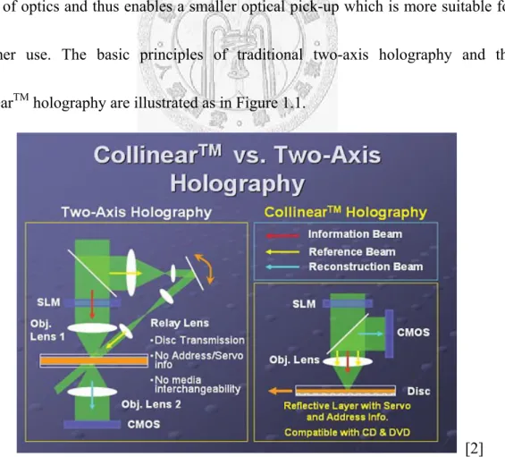
leading scientists at Sony. This company has been developing the HVD systems based on its proprietary Collinear^TM holography. Conventionally, the implementation of most holographic data storages requires two laser beams of different incident angles, which usually leads to highly complex optical systems to line them up at the exact point at which they are supposed to intersect. At the same time, this feature results in the incompatibility with the common CD and DVD systems. Therefore, the Collinear^TM technique suggests a system in which the laser beams travel in the same axis and strike the recording medium at the same angle. This method requires a less complicated system of optics and thus enables a smaller optical pick-up which is more suitable for consumer use. The basic principles of traditional two-axis holography and the Collinear^TM holography are illustrated as in Figure 1.1.

[2]

Figure 1.1 Collinear^TM holography and the traditional two-axis holography

Besides its own continuous development, in 2005 Optware Corp. founded the HVD FORUM (previously named as HVD Alliance), which is a coalition of corporations, intending to provide an industry forum for testing and technical discussion of all aspects of HVD design and manufacturing. As of February 2006, the HVD forum consists of corporations including Optware Corp., CMC Magnetics Corp., Fuji Photo Film Company, LiteOn Technology, etc. They have been working on the standardization of holographic data storage system with the Technical Committee 44 (TC44) of Ecma international, which is an international private standards organization for information and communication systems.

Originally, the HVD format is claimed to be able to store up to 3.9 Terabytes.

Then, Optware was expected to release a 200 GB disc in early June 2006. However, there have been no further news or products on market since the announcement. It seems that the HVD FORUM, led by Optware Corp., is gradually showing less influence in this field, while its competitor, InPhase Technologies may start to dominate.

InPhase Technologies was founded in 2000 as a Lucent Technologies venture, spun out from Bell Labs research. This company also promises Terabyte storage eventually, as Optware Corp. does. At present it has devised a three-stage product roadmap, as shown in Figure 1.2, and the first generation of product, tapestry^TM300r is

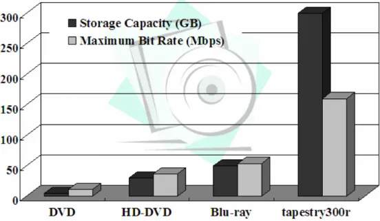
expected to be available on market by the 4^th quarter of 2007. This initial commercialized version is already able to hold up to 300 GB, which is 462 times the capacity of a CD-ROM, 64 times the capacity of a DVD, 10 times the capacity of a dual-layer HD-DVD disc, or 6 times the capacity of a dual-layer Blu-ray disc. In addition to the huge capacity, the throughput rate of tapestry^TM300r also greatly exceeds that of other current optical storages. A comparison of storage capacity and the throughput rate has been provided in Figure 1.3.

At present, the major partners of InPhase Technologies include Hitachi Maxell, ALPS Electric, DisplayTECH, etc. With the commercialization of tapestry300r, we believe that more corporations will join this camp.

[3]

Figure 1.2 Product roadmap of InPhase Technologies (WORM: Write Once Read Many, HDS-300R is the old name for tapestry^TM300r)

Figure 1.3 Comparison of the existing optical storage technologies

1.2 Motivation of Thesis

The successful commercialization of holographic data storage will depend on the cooperation of diverse research fields, including material science, laser optics, drive technology, signal processing, and so on. Among many scopes, this thesis is intended to focus on the aspect of digital signal processing.

Though targeting entirely different applications, an extreme similarity is observed between a data storage system and a wireless communication system. Storing and retrieving information in a data storage system is exactly analogous to transmitting and receiving signals in a communication system. While the channel in a wireless communication system may be the atmosphere, that in a storage system becomes the optical path and the recording medium. Based on experiences in communication

systems, now we plan to apply, with some adaptations, some of those powerful signal processing techniques often used in wireless communications to the optical storages.

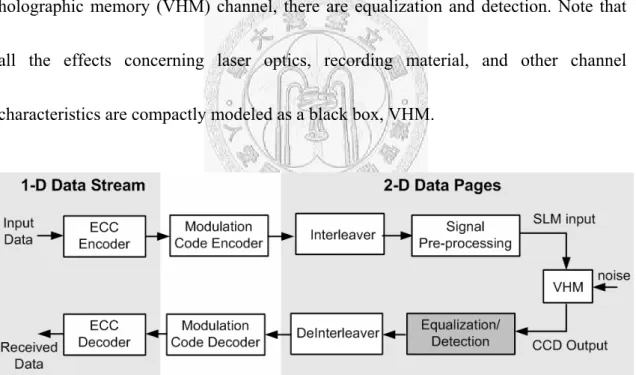
Similar to the approach in defining a communication system, a block diagram is shown in Figure 1.4 to depict a holographic data storage system from the view of digital signal processing. As can be seen, the system includes error-correcting code (ECC), modulation code, the interleaving scheme, and signal pre-processing, whose purpose is to simplify equalizer design. Furthermore, directly following the volume holographic memory (VHM) channel, there are equalization and detection. Note that all the effects concerning laser optics, recording material, and other channel characteristics are compactly modeled as a black box, VHM.

Figure 1.4 Block diagram of holographic data storage system from the view of digital signal processing

Among all the functional blocks, the focus of this thesis is further specified to be on the part of data detection. The aim of data detection is to recover the signal that is

corrupted by inter-pixel interference (IPI) introduced in VHM channel, which may be comparable to the inter-symbol interference (ISI) in wireless communications. The difference is that IPI possesses a two-dimensional nature and normally constitutes a significantly severer threat to signal fidelity, which implies the need for an effective two-dimensional detection scheme, possibly an extension from the one-dimensional techniques applied in wireless communications. Generally, the extent of IPI closely relates to the storage density, and denser data packing usually corresponds to severer IPI. In a sense, a powerful detection scheme will then justify the high-density implementation, and thus further raise the storage capacity achievable.

Another consideration is that powerful detection schemes ordinarily incur higher computational complexity, which will be reflected upon the decreased throughput rate.

Hence, in this thesis, we will focus on the design of an effective detection scheme with reduced computational complexity. The proposed scheme is expected to offer a solution as an enhancement of the next-generation optical storage system.

1.3 Organization of Thesis

The contents of this thesis are organized as follows: Before getting into the design of detection schemes, our assumption about the black box VHM has to be clarified. In Chapter 2, two kinds of channel models that are commonly applied are introduced.

These channel models constitute the basis for the following detector design. In Chapter 3, two iterative detection schemes are presented and compared, and the conclusion is reached with the adoption of the soft detection scheme, 2D-MAP, because of its superior bit-error rate (BER) performance. However, the extraordinary performance is achieved at the cost of a huge amount of arithmetic operations. Therefore, a suite of schemes are proposed to reduce the computational complexity of 2D-MAP detection in Chapter 4. These schemes are targeted for different dimensions of the 2D-MAP algorithm, while combined together, they would be able to realize significant complexity reduction. Based on these schemes, the implementation of the basic processing element in a 2D-MAP detector is proposed in Chapter 5. Some other implementation issues are also discussed in this chapter. Finally, the conclusion and outlook are given in Chapter 6 to end this thesis.

Chapter 2

Introduction to Holographic Data Storage Systems

2.1 Introduction

Similar to a book comprising many pages, the holographic data storage superimposes many so-called holograms in the same position on storage medium through angular multiplexing. A hologram is a recording of the optical interference pattern that forms at the intersection of two coherent optical beams. To make the idea more vivid, the working principle of holographic data storage could be demonstrated with the operation of recording and retrieval of data on a holographic disc:

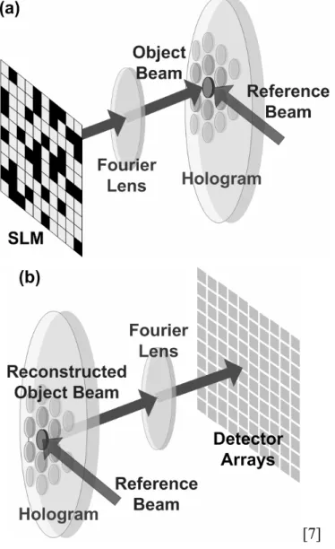
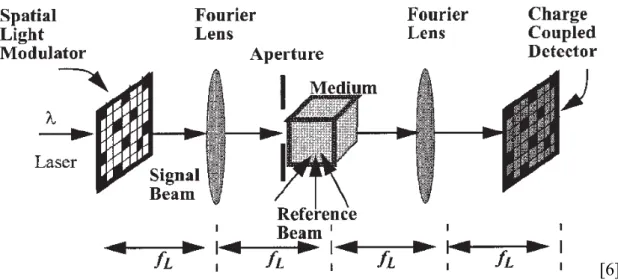
(a) Recording: As shown in Figure 2.1(a), the aforementioned two optical beams are referred to as the object beam and the reference beam. Data taking the form of two-dimensional binary patterns become the object beam after passing through spatial light modulator (SLM) and the Fourier lens. And the reference beam is usually designed to be simple to reproduce. A common reference beam is a plane wave: a light beam that propagates without converging or diverging. When the object beam and a corresponding reference beam overlap with each other on the

holographic medium, the interference pattern between the two beams is recorded.

When the next data page comes in, a second hologram could be stored in the same location only by tilting the incident angle of the reference beam by a small degree.

(b) Retrieval: By illuminating the storage medium with the reference beam of a proper incident angle, a certain object beam is reproduced and then captured by the detector arrays at the receiving end, as clear illustrated in Figure 2.1(b).

[7]

Figure 2.1 In the holographic data storage system: (a) the recording process (b) the retrieval process

By the recording and retrieving scheme, holographic data storages are able to utilize all three dimensions at high resolution, which justifies its property of being a 3-D volume optical storage.

2.2 Channel Model

Owing to the dense packing of data pixels, holographic data storages have been suffering from severe inter-pixel interference (IPI), which is also the major problem that we wish to overcome. To demonstrate the significant influence of IPI, first we will need to introduce and clarify the channel model to be applied.

The first channel model that we are going to present is the complete channel model [5][6], which is the most complex model, yet providing the most accurate approximation of a realistic environment. Thus, the complete channel model is usually treated as the simulation of an actual channel. On the contrary, the second model, the incoherent intensity channel model is a simplified version of the former one. It is a linear model and is not generally applicable to all kinds of holographic data storage channel with different parameter settings. Nonetheless, as will be discussed in Chapter 4, a receiver based on the assumption of an incoherent intensity channel model shall enable a simplified design. As a result, the intensity model is included here in our scope to increase completeness.

2.2.1 Complete Channel Model

A schematic diagram of a 4-fL (focal length) holographic data storage system is shown in Figure 2.2. Each of the two Fourier lenses in this 4-fL architecture performs a Fourier-transform operation, so that the light from Spatial Light Modulator (SLM) is imaged onto the Charged Coupled Detector (CCD). The storage of the Fourier holograms instead of image holograms serves a similar purpose as interleaving, in which the information is distributed in a different transformed domain so as to decrease the possibility of burst errors. And the placement of the aperture in the back of the first Fourier lens is to reduce the size of effective recording area on the holographic medium so that storage density could be increased. As the aperture windows the Fourier transform of the signal beam, it also acts as a low-pass filter whose bandwidth

[6]

Figure 2.2 Schematic diagram of a holographic data storage system in the 4-fL architecture

is determined by the aperture width, thus introducing the inter-pixel interference at the same time. One more thing to note about system is that, here we have assumed the system is pixel matched, which means that each of the SLM pixels is imaged onto one CCD pixel. Pixel-matched imaging is favorable in real implementation since it helps the realization of high data rates.

Based on the 4-fL architecture, a channel model could be developed, as is illustrated in Figure 2.3. The important elements in this model will be introduced respectively as follows.

Figure 2.3 Block diagram of a complete channel model

- dij: The input binary data sequence, dij, takes on values in the set {1, 1/ε}. While a pixel ONE takes the value 1, a ZERO pixel takes the value 1/ε, in which ε is the amplitude contrast ratio, i.e., the ratio of amplitudes of the bit 1 and the bit 0. This non-ideal effect is referred to as “the limited contrast ratio of the input SLM”.

- p(x,y): The SLM’s pixel shape function can be formulated as ( , )

x y

(2.1)

p x y

α α

⎛ ⎞ ⎛ ⎞

=

∏

⎜⎝ Δ⎟⎠

∏

⎜⎝ Δ⎟⎠

Where α represents the SLM’s linear fill factor (namely the square root of the area fill factor for a square pixel). The fill factor is the ratio of the area of the active part of a pixel to the total area of a pixel. The symbol Δ represents the pixel width, which is assumed to be same for both SLM and CCD, and

∏ ( )

^x is the unit

rectangular function. Now, the output from the SLM could be expressed as:

( )

( , ) _kl , (2.2)

k l

s x y

=

∑∑ d p x k

− Δ − Δ

y l

Where

k and l refer to the pixel location along the x and y direction.

- hA(x,y): As mentioned earlier, the aperture leads to a low-pass behavior, whose frequency response is represented as HA(fx,fy) in Figure 2.3. The effect of the Fourier transform, HA(fx,fy) , and the inverse Fourier transform combined together is equal to convolving the SLM output with an impulse response, hA(x,y). The width of hA(x,y) is inversely proportional to the frequency plane aperture width.

For a square aperture of width D, the impulse response of the aperture is described

as

( )

^,

( ) ( )

(2.3)

A A A

h x y =h x h y

Where _A( ) sinc

L L

D xD

h x

λ

f

λ

f

⎛ ⎞

= ⎜ ⎟

⎝ ⎠, in which λ is the wavelength of the light, and

f represents the lens’s focal length. And in this way, the counterpart in frequency

L

domain, HA(fx,fy), is an ideal low-pass filter with a cut-off frequency equal to

2 _L

D

λ f

^{so that}

^x _L

1 |f | D

( ) 2λf (2.4)

0 otherwise

A x

H f

⎧ ≤

= ⎨⎪

⎪⎩

The impulse response hA(x,y), or commonly referred to as the point-spread function (PSF), may be the most critical ingredient in the channel model, since it compactly characterizes the extent of inter-pixel interference. Now, the signal through the PSF can be expressed as

( )

( )

( , ) ( , ) ( , )

, ( , )

, (2.5)

A

kl A

k l

kl

k l

r x y s x y h x y

d p x k y l h x y

d h x k y l

= ⊗

⎡ ⎤

=⎢⎣ − Δ − Δ ⊗⎥⎦

= − Δ − Δ

∑∑

∑∑

Where _⊗ represents a 2-D convolution, and h(x,y), which integrate the effects of the SLM pixel shape function and PSF, is referred to as the pixel-spread function (PxSF). From (2.1) and (2.5), it could be observed that the extent of IPI also depends on the SLM fill factor. A high SLM fill factor would broaden the PxSF, while a low one tends to increase the PxSF roll-off.

-

∫∫

| |^{i 2}: The CCD is inherently a square-law device and tends to detect the intensity of incident light. It transforms the signal from the continuous domain to the discrete domain by integrating it spatially. Thus, the output from the CCD

detector combined with the noises can be described as below:

( 2) ( 2) 2

( ) ( )

2 2

( , ) ^{i j} | ( , ) _o( , ) | _e( , ) (2.6)

i j

Z i j r x y n i j dydx n i j

β β

β β

+ Δ + Δ

− Δ − Δ

=

∫ ∫

+ +

Where

β

represents the CCD linear fill factor. Now we know that the CCD fill

factor also has some connection with the extent of IPI. As a high CCD fill factor normally implies higher signal levels, it also contributes to channel nonlinearity and results in more IPI. And no

(i,j) and n

e

(i,j) represents the term of optical noise

and electrical noise respectively. Optical noise results from optical scatter, laser speckle, etc., and is generally modeled as a circularly symmetric Gaussian random process with zero mean and variance No. Electrical noise arises from the electronics in the CCD array, and is normally modeled as a additive white Gaussian noise with zero mean and variance Ne.

In Summary, the complete channel model is formulated as:

( )

( 2) ( 2) 2

( ) ( )

2 2

( , ) | , ( , ) ( , ) |

( , ) (2.7)

i j

kl A o

i j

k l

e

Z i j d p x k y l h x y n i j dydx

n i j

β β

β β

+ Δ + Δ

− Δ − Δ

⎡ ⎤

= ⎢⎣ − Δ − Δ ⊗⎥⎦ +

+

∫ ∫ ∑∑

There are still a few imperfections in a holographic data storage channel that are not considered, such as the inter-page interference, lens aberration, misalignment (including magnification, tilt, rotation, and translation differences) between SLM and CCD, and so on. However, these effects are either beyond the scope of our research or

could be conveniently integrated with the above architecture, so they are not specifically mentioned earlier. In addition, these effects are regarded as having minor influences when compared to the inter-pixel interference and noises.

For the simulations, pages of size 512×512 pixels are applied, with the parameters:

λ ,

f , and

L

Δ

, set as 515 nm, 89 mm, and 18 μm, respectively. These parameters are

selected as the same as in a paper on the IBM DEMON system [8].

To facilitate adjustment on operating conditions and make the simulation independent from λ ,

f ,

L

Δ

, and D, the normalized aperture width, w, is defined as

N

w D

=

D

, in which _N

f

^L

D

₌

λ

Δ is the Nyquist aperture width. To make the description of the extent of IPI even more intuitive, the normalized half-blur width, W, of the point-spread function (PSF) is introduced and defined as

D

_N 1

W

=

D

= . Thus, W = 1

w

corresponds to a system with Nyquist aperture width, which also implies a system with critical sampling so that the first zero of PSF coincides with the center of the nearest pixel. While a larger W corresponds to severer IPI, a W larger than 1 suggests operation beyond the classical resolution limit.

For simplicity, the amplitude contrast ratio (ε), the SLM fill factor (α ), and CCD fill factor (

β

) are all set to 1 in the simulation. In fact, their influences can somehow

be depicted through the adjustment of W. For the setting of the noises, it is observed in [6] that the system under an electrical-noise-dominated condition and that under an

optical-noise-dominated condition yield extremely similar simulation results, so, again, for the reason of compactness, we choose to consider only the case when electrical noise dominates. We use signal-to-noise ratio (SNRe) to characterize the extent of electrical noise, and it is defined as SNRe=10 log10(0.5²/N0).

Finally, we define two channel conditions that apply the complete channel model in our simulations hereafter: CH-1, with W = 1, represents the case of medium IPI, and CH-2, with W = 1.25, represents the case of severe IPI.

2.2.2 Incoherent Intensity Channel Model

The incoherent intensity channel model is a simplified and linearized version of the complete channel model. It is named “intensity model” because it assumes linear superposition in intensity during image formation, as is shown in Figure 2.4. Besides, the operation of this model on data pages is entirely in the discrete domain; that is, the minimum operating unit is the pixel, as opposed to finer sub-pixel grids that are applied in the complete model. Basically, we can say that the effects of the SLM pixel shape function, the PSF, and the CCD detector have been integrated within one single channel IPI matrix, as is similar to the case for traditional inter-symbol interference (ISI) channel commonly applied in communication systems.

Figure 2.4 Block diagram of the incoherent intensity channel model

Considering an N×N pixel detector array, the system is modeled as linear and shift-invariant, so that it is formulated as: (The index is omitted for simplicity.)

(2.8)

Z

= ⊗ +

A H N

Where Z, A, and N are N×N pixel matrices that represent the page being received, the page being sent, and the additive white Gaussian noise (AWGN) with zero mean and variance N0, so that the SNR of the received page could be defined as SNR=10 log10(0.5²/N0). H represents the IPI, and _⊗ is a 2-D convolution. To be more specific,

H is a 3×3 IPI matrix constructed from a continuous PSF, which is defined here as:

2 2

( , ) sinc

x

sinc

y

(2.9)

h x y

W W

⎛ ⎞ ⎛ ⎞

= ⎜⎝ Δ⎟⎠ ⎜⎝ Δ⎟⎠

Where W is the normalized half-blur width as is defined earlier for the complete model.

Then H is derived from its continuous counterpart (2.9) as:

( 1/ 2) ( 1/ 2) ( 1/ 2) ( 1/ 2)

( , ) ^{i j} ( , ) (2.10)

i j

H i j

^{+ Δ + Δ}

h x y dydx

− Δ − Δ

=

∫ ∫

The size of H will be truncated as that H(i,j) = 0 for |i|, |j |> 1. Finally the remaining

nine coefficients are re-normalized so that they sum up to be one.

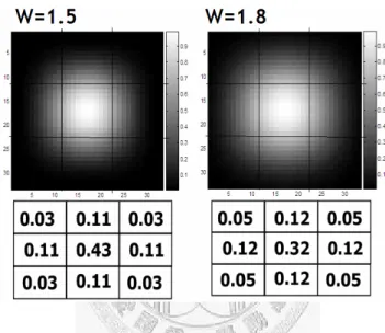
In our simulations, as in the case of complete channel model, two kinds of IPI conditions are set: CH-1, with W = 1.5, represents the case of medium IPI, and CH-2, with W = 1.8, represents the case of severe IPI. The PSF and IPI matrix corresponding to each case are shown in Figure 2.5.

Figure 2.5 The PSF and IPI matrices under the two different IPI conditions

Though less accurate than the complete channel model, the incoherent intensity model is, however, the model usually assumed. [11]-[16] According to [5], the intensity model is an appropriate assumption when the holographic data storage system has high fill factors, so the application of this model can still be justified for some category of holographic data storages. On the other hand, if other page-oriented memories are taken into consideration, this model exactly characterizes the case for an

incoherent optical system, such as the two-photon memory. [9][10] As a result, we have also included the incoherent intensity channel model in our simulations. We have to say that, a final reason is we believe the adoption of intensity model could help inspire some innovations owing to its linearized hypothesis with respect to channel.

This belief will be proved in Chapter 4 that the intensity model does enable a simpler design for the receiver.

A final remark about the channel models is that the application of sinc function in PSF is actually justified by the assumption of a square aperture. However, a square aperture is difficult to acquire in practice, and a circular aperture may be adopted most of the time. Theorectically, the PSF shall then be defined with the polar coordinate, but this increases computational complexity since the convolution with input page is defined in Cartesian coordinate system. Fortunately, we found that, as the PSF is described in the sub-pixel domain, the more sub-pixel into which a pixel is segmented, the more a square aperture resembles the circular aperture. This is shown in Figure 2.6.

When a pixel is segmented into 11×11 sub-pixels, the PSF already looks like resulting from a circular aperture. Furthermore, we compare the channel coefficients derived

from these two sorts of aperture shape by defining D as 20 log₁₀ ^{| |}

| |

circular square circular

H

H H

⋅ −

∑ ∑

^.

Through calculation, we found D is about 56 dB, indicating that the difference between

applying these two assumptions of aperture shape is negligible.

(a) Square Aperture ( =1△ 1) (b) Circular Aperture

Figure 2.6 Comparison between square aperture and circular aperture

2.3 The Impact of Inter-Pixel Interference

Based on the system model described above, our aim is clear: to recover the original pages from the corrupted pages. Owing to IPI, the bit-error-rate (BER) performance achieved by a simple threshold detection, which compares a received pixel value to a fixed threshold and makes the decision, is simply not acceptable, as can be observed in Figure 2.7 and Figure 2.8, which assume the complete channel model and the incoherent intensity channel model respectively. Therefore, a more powerful detection scheme has to be devised.

On the other hand, the optimal detection scheme would be maximum likelihood page detection (MLPD). A conceptually simple method of accomplishing it involves the use of a look-up table (LUT) storing the expected received pages of all possible

data page patterns, with the data page pattern as index. Then an arbitrary received page is compared against every element in LUT to determine the most possible page that

Figure 2.7 BER performance of simple threshold detection under the complete channel model

Figure 2.8 BER performance of simple threshold detection under incoherent intensity channel model

was recorded. However, this is not even feasible, since a system with N×N pixel pages would require a LUT with 2^N×N entries, as is illustrated in Figure 2.9.

While there is no practical implementation for MLPD at present, we are going to pursue the sub-optimal detection schemes.

Figure 2.9 The MLPD requires the examination of all possible combinations of data page pattern

Chapter 3

Iterative Detection Schemes

3.1 Introduction

Since there is no feasible implementation for MLPD at present, the sub-optimal detection schemes are being pursued. The iterative detection schemes aim to approximate the idea of MLPD by iteratively making improvements on their decisions.

Two representative schemes are parallel decision feedback equalization (PDFE) [12]

and two-dimensional maximum a posteriori (2D-MAP) detection [13], as PDFE being a hard detection scheme and 2D-MAP detection being a soft one, so that some insights shall be inspired from the demonstration and comparisons of these two extremes of approaches. In following discussions, we will assume a perfect knowledge of the channel information, in order to put our focus on the detection at receiving end.

3.2 Parallel Decision Feedback Equalization (PDFE)

As a hard detection scheme, in each iteration, PDFE makes a hard decision at each pixel, based on the knowledge of the decisions of the corresponding eight neighbors in last iteration.

To be specific, this detection scheme can be explained by two steps of operation:

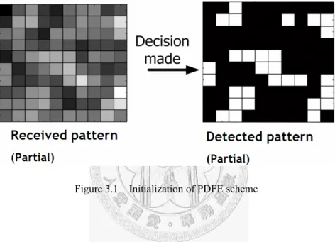
(a) Initialization: The hard decisions are made on all pixels with respect to a fixed threshold, as is clearly illustrated in Figure 3.1. Thus, in the detected page pattern, every pixel has been assigned a binary value to be either “1” or “0”.

Figure 3.1 Initialization of PDFE scheme

(b) Hard decision feedback: For every pixel, given the decisions from its neighbors together with the channel information, the expected pixel value (namely, the noise-free channel output) given that it is sent as a “1” (Z1), and given that it is sent as a “0” (Z0), can be computed. Then, a pixel is decided to be “1”, if

|Z(i,j)-Z1|<|Z(i,j)-Z0| (where Z(i,j) represents the received pixel value); otherwise, it is decided to be “0”. The procedure is executed simultaneously at all pixels on the page, and then all updates of hard decisions also take place simultaneously in

the end of each iteration. This step is iterative and will repeat itself until no further change of hard decisions in the detected page, or a predetermined iteration number is reached. In practice, the BER normally converges in no more than 3 iterations.

This step is illustrated in Figure 3.2, where Nij represents the corresponding neighborhood pattern of the current pixel. The incoherent intensity model is assumed here, so the channel information is represented by a 3×3 IPI matrix.

Figure 3.2 Hard decision feedback of PDFE scheme

3.3 Two-Dimensional Maximum A Posteriori (MAP) Detection

Two-dimensional maximum a posteriori (2D-MAP) detection, which was proposed in [13] as the 2D⁴ (Two-Dimensional Distributed Data Detection) algorithm, is actually the well-known max-Log-MAP algorithm. As opposed to the hard decision

in PDFE, the information kept by each pixel is a log-likelihood ratio (LLR), or more intuitively, a reliability value that indicates its probability of being “1” and being “0”.

To be specific, an LLR with a more positive value indicates a greater probability of a pixel to be a ‘0”, and a more negative LLR indicates a greater probability for it to be a

“1”. Following the same reason, an LLR value which is around zero then indicates that the decision concerning current pixel is still somewhat ambiguous. In each iteration, the reliability value at each pixel will be re-calculated, based on the knowledge of LLRs of the nearest neighbors in last iteration.

Again, to delve into the details of this algorithm, 2D-MAP detection could also be explained by steps:

(a) Likelihood feedback: Under the current assumption of equal a priori statistics (i.e., P[A(i,j)=1]=P[A(i,j)=0]), the MAP rule actually reduces to the maximum likelihood (ML) rule. If we use Nij to represent a set of neighboring pixels that surround pixel (i,j), and use Ω to represent the set of all possible combinations of neighborhood patterns, then for every pixel, the likelihood is calculated via:

[ ( , ) | ( , )]

{ [ ( , ) | ( , ), ]}

[ ( , ) | ( , ), ] [ ]

[ ( , ) | ( , ), ]( [ ( , )])

ij

ij

N ij

ij ij

N

ij

P Z i j A i j

E P Z i j A i j N P Z i j A i j N P N

P Z i j A i j N P A l m

∈Ω

=

=

= Π

∑

∑

(3.1)

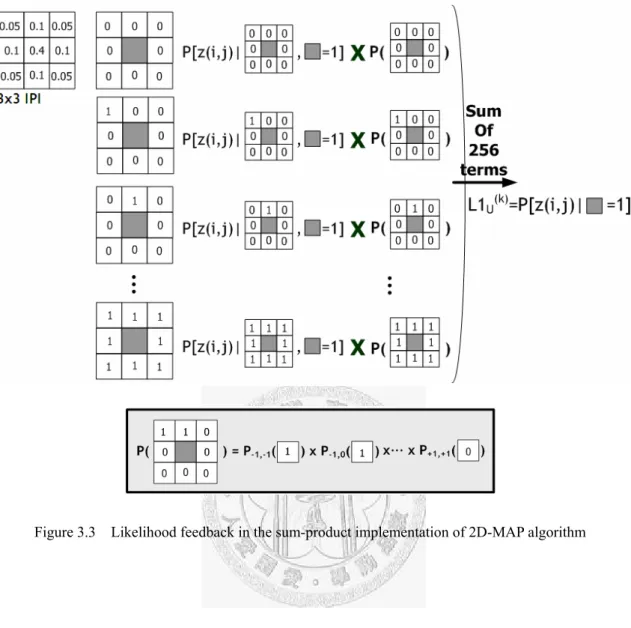
Note we have assumed that a pixel is independent of one another, so that the probability of a neighborhood pattern can be calculated by multiplying all the component pixel probabilities together. Ideally, the expectation in (3.1) shall be taken over the entire page, so that MLPD is achieved. Such a task is computationally unreasonable, while computing the bit likelihood based on a subset of the observation page is feasible. Then, information shall be spread through iterations, and MLPD could be approached. Here, a more concrete demonstration of (3.1) is provided in Figure 3.3, and the aforementioned subset is simply a 3×3 region surrounding the current pixel being detected.

In Figure 3.3, the calculation of a bit likelihood is shown. Note that the final result of this computation is denoted as L1U, where “1” means that it is the likelihood under the hypothesis that the current pixel is sent as a “1”, and the subscript “U” means that this likelihood is an updating term for the likelihood calculated in last iteration. We distinguish L1U from L1, because L1 would not be directly replaced by L1U. This would become clear after the explanation of the second step in 2D-MAP detection.

Given the channel information, all the 2⁸=256 neighborhood patterns are concerned in the calculation of this summation of conditional probability.

One more critical element to complete this step is the a priori probabilities, which are intended to be involved in the computation of the probability of a neighborhood

Figure 3.3 Likelihood feedback in the sum-product implementation of 2D-MAP algorithm

pattern. Actually, the likelihood P[Z(i,j)|A(i,j)] can be thresholded to make a decision based solely on Z(i,j). Nonetheless, a significantly more reliable decision will result from a likelihood considering other observations too. As a result, [13] suggested to infuse the likelihood information from neighboring pixels by applying (3.1) with P[A(l,m)] substituted by P[Z(l,m)|A(l,m)]. The replacement of a priori probabilities by the likelihood values acquired in last iteration is known as the propagation of extrinsic information, which is commonly used for turbo decoding. By this replacement, the

structure of an iterative detection is established. Note that the propagation of extrinsic information also deprives the pixel probabilies of their independence, which is the reason for 2D-MAP algorithm being not optimal.

As demonstrated with (3.1) and Figure 3.3, we know that a huge amount of multiplications and additions are involved. As is typically addressed, this is a sum-product implementation of MAP algorithm. In practice, motivated by the

approximation [17],

( ) ^{( )}

log

∑

_i

X

_i ≈ max log(_i

X

_i) ^(3.2)

the min-sum approach is adopted as in (3.3).

{ }

( ) ^{( )}

( , )

log [ ( , ) | ( , )]

min log [ ( , ) | ( , ), ] log [ ( , )] (3.3)

ij ij

N ij

A l m N

P Z i j A i j

P Z i j A i j N P A l m

∈Ω ∈

−

⎧ ⎫

⎪ ⎪

= ⎨− + − ⎬

⎪ ⎪

⎩

∑

⎭

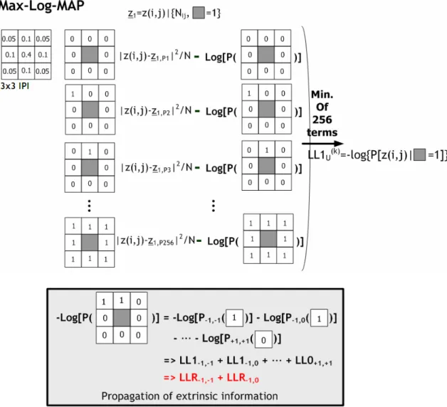
The first term in (3.3) is actually the normalized squared Euclidean distance, and the second term is supposed to be a sum of log-likelihoods. Once again, a more concrete demonstration of this implementation of 2D-MAP has been provided, as in Figure 3.4.

In Figure 3.4, z1,P represents the expected received pixel value given a sent “1”

and a certain neighborhood pattern, and the final computation result LL1U represents an updating term for the log-likelihood value. As can be seen, calculating the summation of 256 product terms as in Figure 3.3 has been replaced by finding the minimum among the 256 sum terms, which is a significant reduction in computation.

In the calculation of the second term in (3.3), each logarithm of a priori

probability is substituted by the corresponding log-likelihoods, which was referred to as the propagation of extrinsic information earlier. To be specific, P[Z(i,j)=1] will be replaced by LL1(i,j), and P[Z(i,j)=0] will be replaced by LL0(i,j). Now, suppose that for all the neighborhood patterns considered for the current pixel, the eight LL0s are subtracted from the original sum of log-likelihoods. This operation results in an equal

Figure 3.4 Likelihood feedback in the min-sum implementation of 2D-MAP algorithm

shift of the value of LL1U and LL0U, and after the introduction of step two in 2D-MAP algorithm, we will know that this equal shift does not make any differences with respect to the detection results. Therefore, another way to calculate the second term in (3.3) is suggested: we only include LLR(i,j) in the summation if Z(i,j)=1 in the hypothesis of the neighborhood pattern, as the example shown in the lower part of Figure 3.4. In this manner, half of the addition operations are saved on average. Then the equation (3.3) could be adjusted to become:

( ) 2 ( 1)

, ( , ) ( , )

0

( , ) min 1 | ( , ) ( ) | (3.4)

2

k k

U X i j X X i j

LL i j Z i j H X L X

N

+ −

⎧ ⎫

= ⎨ − + • ⎬

⎩ ⎭

Where the term in the left hand side represents the updating term for log-likelihood being calculated in k-th iteration, given a hypothetical sent value, X+X(i,j) represents a 3×3 pixel pattern, with pixel (i,j) as the center, X represents X+X(i,j)－{X(i,j)}, and L^(k-1) is the corresponding LLR matrix in (k-1)-th iteration. The symbol․represents an inner

product of two matrices. Note that H(X+X(i,j)) is the black-box function of expected channel output given a 3×3 pattern X+X(i,j). In the incoherent intensity channel model, the content of this function could be further specified as the inner product between a known IPI matrix and X+X(i,j), that is, H․X+X(i,j).

(b) Update: Updating of LLRs is executed at the end of each iteration. To avoid

abrupt changes in updated LLR values, a forgetting factor is applied in updating as

{ }

( ) ( 1) ( ) ( )

, ( , ) 1 , ( , ) 0

( , ) (1 ) ( , ) ( , ) ( , ) (3.5)

k k k k

U X i j U X i j

L i j

= −

β L

⁻

i j

+

β LL

₌

i j

−

LL

₌

i j

The choice of β concerns the trade-off between speed of convergence and accuracy of the converged results. A larger β may lead to faster convergence but possibly inferior performance. To determine β and number of iteration needed, the simulations are made according to the two different hypotheses about channel:

<1> the complete channel model

In order to observe the converging behavior with respect to different β value, we have plotted the BER against the number of iterations for different choices of β under adequate SNR settings for CH1 and CH2, as is shown in Figure 3.5. For deeper interpretation, two extra plots are provided in Figure 3.6, in which the upper plot shows the iteration number required to reach 10^-3 BER versus β, and the lower plot shows the converged BER versus β; a lower iteration number to reach 10^-3 BER indicates a faster convergence, and a lower converged BER indicates a better converged performance. Our goal here is to find a β value that strikes a balance between the convergence rate and converged performance. The upper plot in Figure 3.6 points out a suitable range for β to be 0.7-0.8, and the lower plot points out the suitable range for β to be 0.4-0.7. Combined with the concern of iteration number, which can be observed in Figure 3.6, we determine to use β = 0.7 for 15 iterations in our

implementation of 2D-MAP detection.

<2> Incoherent Intensity Channel Model

The same simulations are done for the incoherent intensity channel model. The converging behavior is shown in Figure 3.7, and the indicators of convergence rate and converged performance are shown in Figure 3.8. The upper plot in Figure 3.8 indicates that a suitable β would be 0.7, while the lower plot indicates a suitable range of β to be from 0.3 to 0.8. Combined with the concern of iteration number shown in Figure 3.7, again we decide to apply a β of 0.7 for 20 iterations in the implementation of 2D-MAP detection.

Figure 3.5 BER plotted against iteration number for different β (Complete Channel Model)

Figure 3.6 Iteration number required to reach 10^-3 BER and converged BER plotted against β

Figure 3.7 BER plotted against iteration number for different β (Incoherent Intensity Channel Model)

Figure 3.8 Iteration number required to reach 10^-3 BER and converged BER plotted against β

3.4 Performance Comparison

In this section, the performance of the iterative detection schemes introduced in the chapter is compared, under two different channel models with two kinds of IPI conditions respectively. The comparison under the complete channel model is shown in Figure 3.9, and that under the incoherent intensity channel model is shown in Figure 3.10. The simulation results coincide with our expectation toward these two

approaches. As a hard detection scheme, PDFE sacrifices its performance for simplicity. By merely operating on the hard decisions, lots of information has been neglected, which leads to the inferior performance of PDFE than that of 2D-MAP detection. Furthermore, as the extent of IPI increases, the tendency of showing an error floor is much more obvious for PDFE than for 2D-MAP detection. As a result, in the case of severer IPI, the detecting performance of PDFE is not even acceptable. Based on above reasoning, we have concluded with the adoption of 2D-MAP detection. An unfavorable factor remained would be the high computational complexity associated with the 2D-MAP algorithm. In next section, we shall devise an effective suite of complexity-reducing schemes for a 2D-MAP detector, so that the implementation of it becomes feasible.

Figure 3.9 Performance Comparison of PDFE and 2D-MAP (Completer Channel Model)

Figure 3.10 Performance comparison of PDFE and 2D-MAP (Incoherent Intensity Channel Model)

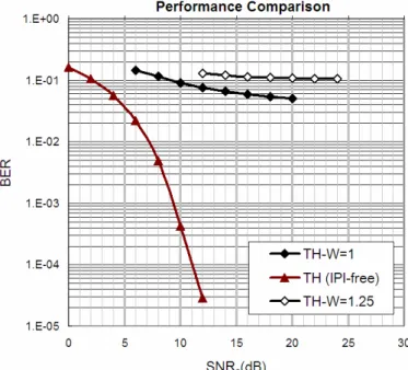
Two final notes about the iterative detection schemes are provided here for completeness. The first one concerns the possibility of extremely severe channel conditions. The case in which W=1.5 is simulated for the complete channel, as is shown in Figure 3.11. Under the circumstance, simple threshold detection and PDFE do not even show any decrease in BER as SNR increases, and the BER curve of 2D-MAP also has a much smaller slope than those with W=1 and W=1.25. This simulation result provides an idea that a W of 1.5 or above may suggest a too harsh channel environment for current iterative detection schemes. Fortunately, the real HDS

Figure 3.11 Performance Comparison including a severer channel condition

channel usually seems milder. As suggested in the channel model recently proposed [6], the range of W is within 0.8-1.25 for complete channel model. Thus, our settings of W as 1 and 1.25 in our simulations seem quite reasonable.

The second note is about our assumption of perfect channel estimation. Here, for the reason of completeness too, a performance simulation considering estimation error is offered. In Figure 3.12, we compared the BER performance under different amount of estimation error. NEE (Normalized Estimation Error) is defined as standard deviation of channel estimation error divided by the output signal mean. A rough idea is thus provided for required accuracy of channel estimation, which is to be included in the future.

Figure 3.12 Performance degradation owing to channel estimation error (W=1.25, Complete Channel)

Chapter 4

Schemes to Reduce Computational Complexity of 2D-MAP

4.1 Introduction

2D-MAP detection offers superior performance under conditions of severe IPI and thus becomes a powerful solution to overcome the two-dimensional crosstalk present in holographic data storage systems. However, the high computational complexity poses a concern for practicality. For demonstration, all the arithmetic operations involved in 2D-MAP detection have been unfolded and illustrated as in Figure 4.1.

During every iteration, the combination of the normalized squared Euclidean distance and the sum of LLRs is calculated for each possible neighborhood pattern, which is normally referred to as candidate. To provide an idea, the number of iterations and candidates are 15 and 256 respectively for our system simulated with the complete channel model. Then, in the calculation of the aforementioned combination, an addition-intensive part would be for the sum of LLRs, in which at most 7 additions are needed to sum 8 LLRs together. Therefore, as is expressed in Figure 4.1, a suite of three complexity-reducing schemes will be presented, with each one of them focusing

on a different dimension of the algorithm.

Figure 4.1 The arithmetic operations involved in 2D-MAP and three aspects on complexity reduction

4.2 The Schemes to Reduce Computational Complexity

In this section, the suite of three complexity-reducing schemes will be introduced respectively, including schemes of iteration reduction, candidate reduction, and addition reduction. For generality, this research architecture has been developed under the complete channel model, which can be seen as equivalent to the actual channel and without extra hypotheses or simplifications.

4.2.1 Scheme of Iteration Reduction

As 2D-MAP algorithm being an iterative detection scheme, the iteration number for the BER to reach a converged state may be different as the channel condition varies.

As could be recalled in Figure 3.5, we only verify the relationship of iteration number and BER performance for a specific SNR setting, since for other SNR values, the relationship can be somehow quite different. Even so, a trend shall be predicted: when the SNR is higher, the iteration number needed to reach convergence will definitely be fewer. While in the previous implementation with a fixed iteration number, in order to keep a design margin, the iteration number we choose may be too large than enough for some channel settings. This is why the idea of an adaptive iteration number comes into play, and thus topics on stopping criteria have been researched. [18][19]

A question naturally appears: how do we know when the iterative detection can be stopped? BER is not a metric that can be conveniently accessed owing to the lack of original information, so we have to search for other metrics that could serve as an indicator for the trend of BER and could be easily obtained at the same time. In previous literatures, there have been a few stopping criteria proposed to terminate the iterative detection at convergence. Examples include the sign-change ratio (SCR) criterion and the hard-decision-aided (HDA) criterion. The SCR criterion counts the sign changes of extrinsic information during the updating step and stops the iteration

when the number of total sign changes decreases under a pre-defined threshold. And the HDA criterion stops the iteration when the hard decisions of a block between two consecutive iterations fully agree. However, in these stopping criteria, the iteration number is set the same for all pixels in a page or a region within a page.

In fact, in the entire page to be detected, there are pixels which converge faster, while others slower. If they are not treated in the same way, the average iteration number is able to be further decreased. Here, the definition for the convergence of pixel may be slightly different from that mentioned earlier for the BER. Previously when we say that the BER has converged, we mean that through iteration the fluctuation of BER curve has become steady. Now when we say a pixel has converged, we mean that the hard decision of that pixel has remained the same and stop alternating between 1 and 0. While telling the stop of alternating is really not easy, is there a more reliable approach to decide that a pixel has converged?

Given the formula of likelihood feedback (3.4), it can be observed from simulation that, as iteration proceeds, the magnitudes of the LLR terms grow larger and larger. This is because, as belief propagates, the decisions are gradually being improved so that the LLR moves toward positive or negative infinity. Through iteration, finally the LLR grows to an extent that the sum of LLRs in (3.4) dominates the entire

min{}.

Note that (3.4) has to be performed for both the hypotheses {X(i,j)=1} and {X(i,j)=0}. Owing to the aforementioned phenomenon, the candidates X that result in the minimum under both hypotheses would eventually become the same one. And when they become the same, this pixel has very likely already converged.

So we can formulate the following Iteration-Reduction scheme in two steps:

I. For every pixel in current iteration, keep tracks of the candidates that result in the minimum for both hypotheses. Let’s name them as ML_Candidate_1 and

ML_Candidate_0.

II. If ML_Candidate_1 = ML_Candidate_0 in successive two iterations, then this pixel will be judged as “converged”. Its LLR will be raised to the extreme value, which may be seen by other neighbors as a decision making. And the detection of this pixel is stopped.

If a pixel still does not reach the “converged” state at the predetermined iteration number (15, as in our case), then the detection on that pixel will be stopped anyway.

Thus the worse case for a pixel would be running the same iterations as our original 2D-MAP scheme without iteration reduction. This above two-step strategy can be illustrated in a flowchart as in Figure 4.2. A counter is kept for each pixel to indicate for how many times the two ML candidates have been the same. With this scheme, different iteration number would be associated with different pixels. In Figure 4.3, we

Figure 4.2 Flowchart of the iteration-reducing scheme

Figure 4.3 Iteration number adaptive to SNR