Automatic Traffic Surveillance System for Vision–Based Vehicle Detection and Tracking

(1)

Automatic Traffic Surveillance System for Vision–Based Vehicle Detection and Tracking

Chung-Cheng Chiu Min-Yu Ku Shun-Huang Hong Chun-Yi Wang Jennifer Yuh-Jen Wu* Hsia Li*

Department of Electrical and Electronic Engineering Chung Cheng Institute of Technology, National Defense University

*Ministry of Transportation and Communications, Institute of Transportation

chiu@ccit.edu.tw g980303@gmail.com luckmouse@gmail.com g951301@ccit.edu.tw

Abstract

This manuscript proposes a real-time system to detect, recognize, and track the multiple vehicles on the roadway images. The system uses an image capture system to snap a sequence of images and a moving object segmentation method to separate the moving vehicles from the image sequences. After the segmentation of the objects, the objects can be classified and counted by the proposed detection and tracking methods respectively. In this system, the occlusive problems are solved by the proposed occlusive segmentation method and then each segmented vehicle is recognized according to their outlines and tracked by a tracking algorithm at the same time. Even though the occlusive vehicles appearing in the images have been keeping merging or having more than two vehicles to merge together all the time, the system can still segment the vehicles. The proposed recognition method uses the visual length, visual width, and roof of vehicles to classify the vehicles to vans, utility vehicles, sedans, mini trucks, or large vehicles. Experiments obtained by using complex road scenes are reported, which demonstrate the validity of the method in terms of robustness, accuracy, and time responses.

Key-Words: Vehicle, Visual, Recognition, Tracking, Occlusive, Segmentation.

1 Introduction

The researches of the intelligent transportation system (ITS) become very popular including vehicle detection, vehicle recognition, vehicle counting and traffic parameter estimation, etc. Due to the upcoming low cost hardware and the progress in algorithmic research, computer vision has become a promising base technology for traffic sensing systems. The vision sensor provides more information than conventional sensors widely applied for using in the ITS. Therefore, some

researches are attracted to the topic of the vision- based traffic surveillance system.

Background extraction offers well pre-processing for the traffic observation and surveillance. It reduces the insignificant information of the image sequences and speeds up the processing time. To reduce the computing complexity, many approaches are proposed to segment the video image into background image and moving object image. The background image is motionless over a long period of time, and the moving object image only contains the objects which are in front of the background.

The change detection [1][2] is the simplest method to segment moving object. An adaptive background update method [3] is proposed to obtain the background image over a period time. He et al. [4]

use the Gaussian distribution to model each point of background image. It uses the mean value of each pixel during a period time as the background image.

Stauffer et al. [5] [6] [7] utilize spectral features (distributions of intensities or colors at each pixel) to model the background. In order to adapt different illumination changes, some spatial features are also exploited [8] [9] [10]. These methods can obtain background images over a long period time. Chiu et al. [11] uses the statistical algorithm to obtain the color background and moving objects efficiently. It can obtain better background image than the methods mentioned above. In this manuscript, we use the statistical algorithm [11] to extract the background image.

As the well background image is obtained the moving object can be detected by subtracted the background image from an input image. After the moving object detection, the next step is to detect and segment the occlusion vehicles from the moving objects. The problem of vehicle occlusion can cause defects in calculating traffic flow parameters and recognizing vehicles. So how to solve the vehicle occlusion is a stimulating task for researchers of the

(2)

intelligent transportation system (ITS). Pang et al.

[12] work on the cubical model of the foreground image to detect occlusion and separate merged vehicles. Method described in [13] utilizes vehicle shape models, camera calibration, and ground plane knowledge to detect, track and classify moving vehicles in presence of occlusion.

However, these methods are time-consuming, and can’t handle the real-time application. In the system, an occlusion detection and segmentation method are proposed to solve the vehicle occlusion in real-time.

The following step is to recognize the classification of the moving objects. Several works consider the problem of object recognition in the shapes and topological structure [2][14][15]. Vehicle recognition using shape model has been demonstrated with encouraging results. However, these recognition methods are incapable for real- time issue. Vehicle recognition and tracking methods are also proposed to recognize vehicles in real-time.

2 Overview of the proposed system

The flowchart of the real-time vehicle recognition and tracking system is shown as Fig.1. The first phase is to segment the moving objects. In this work, we use the statistical algorithm [11] proposed by Chen et al. to extract the background image. The moving objects are detected by subtracting the background image from the input image. Then, the moving objects are processed by the connected component labeling method [16] to obtain the bounding boxes. These occlusive vehicles will be detected and segmented in the bounding boxes. We propose an effective method to detect and segment the different kinds of occlusive vehicles from their shape characteristics. It could segment two or even more vehicles which were occluded by each other.

Finally, the recognition and tracking methods will be processed to each vehicle. The system can classify five types of vehicles, and detect the traffic flow and the average speed.

3 The Definitions of the Visual Length and Visual Width

The dimensions of a vehicle are important parameters because the length and width of different vehicles are distinguishable. Because the unit of the length in the image plane is pixel, the pixel length of a vehicle is different according to the position of the vehicle in the image plane. We have to compute the actual length of the outline of a vehicle, no matter where the position of the vehicle is. Therefore, this

study defines the visual length and visual width of each vehicle style to approach the actual length and width of the vehicle, and proposes a vehicle recognition method with the visual length and visual width of a vehicle.

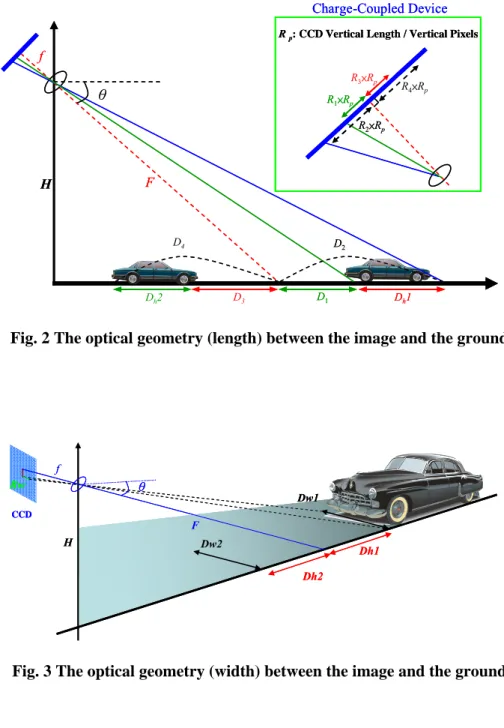
Using the optical geometry to find the relations between the pixel length, R, in the image plane and the visual length, Dh1, on the ground shows as Fig.2.

The dotted line, F, is the central line of the CCD camera and the Dh1 is the visual length of the vehicle above the dotted line F. The R₂ and R₁ are the pixel lengths in the image plane, and the R_p is the pixel size of the CCD camera. The H is the altitude of the camera, the f is the focus of the lens, and the θ is the pitch angle of the camera.

According to the altitude and the pitch angle of the CCD camera, the relation between H and F is

θ sin

F= H (1) By the definition of the similar triangles, the relation of the lengths, D₁ and D₂, are shown as Eq.2 and Eq.3.

θ θ cos sin

1 1 1

D F

D f

R R _p

= + (2) θ

θ cos sin

2 2 2

D F

D f

R R _p

= + (3) Substitute Eq.1 into Eq.2 and Eq.3, the lengths, D₁ and D₂, can be respectively expressed as Eq.4 and Eq.5.

⎟⎟

⎠

⎞

⎜⎜

⎝

⎛

= −

θ θ

θ cos sin sin cos

sin ₁

1 1

p p p

p

R R f

R H R

R R f

F R D R

(4)

⎟⎟⎠

⎞

⎜⎜⎝

⎛

= −

θ θ

θ cos sin sin cos

sin 2

2 2

p p p

p

R R f

R H R

R R f

F R D R

(5) Then, we can compute the visual length, Dh1, from Eq.6.

⎥⎥

⎦

⎤

⎢⎢

⎣

⎡

− −

= −

−

=

θ θ

θ sin cos sin cos

sin 1

1 1 2

2 1 2

p p

p

R R f

R R

R f H R R

D D Dh

(6) For the same step, the vehicle’s visual length, Dh2, below the focus can be calculated by Eq.7.

⎥⎥

⎦

⎤

⎢⎢

⎣

⎡

− +

= +

−

=

θ θ

θ sin cos sin cos

sin 2

3 3 4

4 3 4

p p

p

R R f

R R

R f H R R

D D Dh

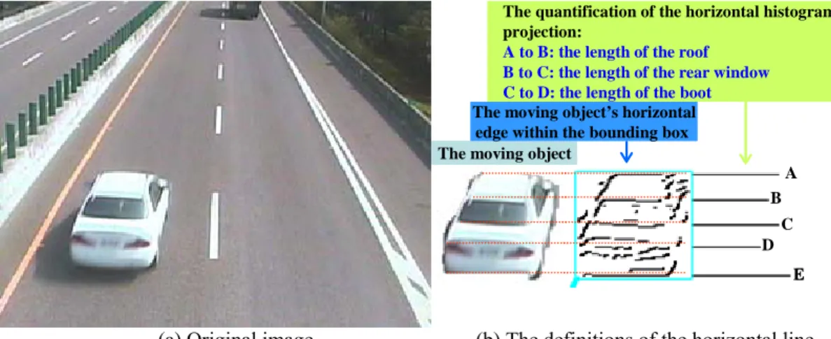
(7) After getting the visual length, we can use the same concept to get the vehicle’s visual width shown as Fig. 3. The visual widths are defined as Eq.8. and Eq.9.

f H D R f Dw

Dh F Rw

Dw ^w ⎟

⎠

⎜ ⎞

⎝

⎛ +

= + ⇒

=

θ θ

θ sin ^cos

cos 1 1

1 ¹

(8)

(3)

f H D R f Dw

Dh F Rw

Dw ^w ⎟

⎠

⎜ ⎞

⎝

⎛ −

=

− ⇒

=

θ θ

θ cos

2 sin cos

2

2 ³

(9) In Eq.8 and Eq.9, the Rw is the pixel width of the vehicle in the image plane. The Dw1 and Dw2 represent the vehicle’s visual width above and below the central line F, respectively.

According the vehicles sold in Taiwan, we calculate the average visual length and width of different cars, including 29 brand names, shown as Table 1. Although the height of a car causes the visual length a slight error, we can still exactly distinguish the style of a car on the road by Table1.

4 Vehicle Recognition method

Because the length and width of a vehicle depend on the model of the vehicle, the preliminary classification is according to the length and width of the vehicle. We will compute the visual length and width of the vehicle outline to implement the vehicle recognition. If the visual length of a moving object is over 12 meters and the visual width is over 3 meters, the moving object will be classified to large vehicle, such as bus or truck. When the visual length of the moving object is between 4.5 to 7.5 meters, and the visual width is between 1.4 to 3 meters, the moving object will be classified to small vehicle, such as van, utility vehicle, sedan, or mini truck. After preliminary classification, the proposed recognition method uses to precisely classify small vehicles. The details are described as below.

4.1. Horizontal edge detection and Quantization The image sequences are snapped from the camera which is amount above the roadway. The direction of the camera is parallel to the direction of moving objects. After the object segmentation, every object will be marked as a bounding box.

Assume the width and height of the bounding box are X and Y, respectively. Firstly, use the Canny method [17] to get the horizontal edge of the object within the bounding box. The Canny mask is obtained by Eq.10.

2 2 2

2 ( ( ) / 2 )

( , ) ( / ) ⁱ ^j , 2

Cy i j = −i σ e⁻ ⁺ ^σ σ = (10) In this work, we use a Canny mask (5×5 pixels, σ=2) to detect the horizontal edge pixels. After the processing of the Canny mask, the width of the horizontal edge is more than one pixel. The non- maxima suppression and hysteresis thresholding [18]

are used to refine each horizontal edge whose width will become one pixel. Then, we count the edge pixels for each row. The projection forms a horizontal histogram which accumulates horizontal edge pixels for each row, shown as Eq.11.

j i i E j

Hy

j i E j

j Hy

Hy ∀

⎩⎨

⎧

≠

=

= + ,

1 ] , [ ],

[

1 ] , [ , 1 ] ] [

[

(11) where i is from 0 to X and the j is from 0 to Y.

The E[i, j] denotes the binary value of each edge pixel. The parameter, Hy[j], is the projection value of each row.

In the captured image, the horizontal edge pixels of the outline of a vehicle will be influenced by the shooting angle which brings the inclination to the horizontal edges. Therefore, the horizontal projection histogram is quantified as follow:

[ ] [ ] [ ] [ ] [ ] [ ]

⎪⎩

⎪⎨

⎧

+

≤

= +

+

= +

+

>

= + +

+

=

1 ,

0 1

1

1 ,

0 1 1

j j j

and j j j

j j j

and j j j

H H H

y j y

y y y

(12) Then, using the threshold value, Tp, selects the significant horizontal projection edges. The method is showed as Eq.13. In this study, Tp is set to 90%

of the first quantified horizontal projection edge of the vehicle.

⎩⎨

⎧

<

= >

Tp j Hy

Tp j Hy j j Hy

Hy 0, [ ]

] [ ], ] [

[

(13) These horizontal projection edges represent the horizontal edges of the vehicle’s roof, windshield, hood, and so on. By using these horizontal projection edges, we can measure the visual lengths of the roof, windshield, and hood of a vehicle. The information can be used to recognize different vehicles.

4.2 Measuring the outline of vehicles

The vertical distance between two neighbor significant horizontal edges represents the visual lengths of the vehicle’s roof, windshield, hood, and so on. The visual length of the roof, rear window, and boot of the vehicle can be computed by the Eq.6 or Eq.7. After the processing of the horizontal edge detection and quantization, the length definitions of the roof, rear window, and boot are described in Fig.4.

By the imaging geometry and the view angle of the CCD camera, we can clearly know that the hood of a vehicle will be covered by the roof of a vehicle in the image plane, so we can define the first line

“A” is the roof of the vehicle. Because different vehicles have different contours, these parameters can be taken as important features for the vehicle recognition. Because the visual length of the roof and the visual width of vehicles are quite different (shown as Table 1), the recognition method only uses the parameter of the roof, Dr, to recognize the vehicles, and the visual width, Dw, of vehicles to recognize the mini truck. We can distribute the small car into mini truck, van, utility vehicle and

(4)

sedan. The classification rule is shown as Eq.14.

Mini Truck 2.2

Van, 2.0

Utility Vehicle, 1.6 2.0 2.2

Sedan, 1.5

Dw m

Dr m

m Dr m Dw m

Dr m

⎧ ≥

⎪⎧ > ⎫

⎪⎨⎪⎨ ≤ ≤ ⎪⎬ <

⎪⎪ ⎪

⎪⎩ < ⎭

⎩

(14)

5 Occlusive Vehicle Detection and Segmentation

In general, not every vehicle in the snapped image can be segmented successfully and alone. If a bounding box contains occlusive vehicles as shown in Fig.5, the occlusive vehicles can not be successfully recognized in this region. Therefore, we have to solve the occlusive problems. From the occlusive images, we can generalize four occlusive situations in a connected component object.

Case 1. Horizontal occlusion: a vehicle merges with the others that are in its right or left side.

Case 2. Vertical occlusion: a vehicle merges with the others that are in the back (or front) of it.

Case 3. Right diagonal occlusion: a vehicle merges with the others that are in the right back of it.

Case 4. Left diagonal occlusion: a vehicle merges with the others that are in the left back of it.

The horizontal occlusion and vertical occlusion can be detected and segmented by the visual length and width of the bounding boxes. The Table 2 is the average visual dimensions of different vehicles.

If the visual width of the object in a bounding box is less than 3.3 meters and the visual length of the object is larger than 7.5 meters, the objects in the bounding box may be classified to case 2, case 3, or case 4. The segmentation steps are described as follows:

Step 1. Count the horizontal projection histogram of the bounding box.

Step 2. Compute the average projection value, Pavg, of the horizontal projection histogram within 3 meters of visual length from the bottom of the bounding box.

Step 3. Calculate the visual width, W_vis, for the average project value, P_avg.

Step 4. According to the values in Table 2, use the visual width, W_vis, to find the best matched model of the vehicle and its visual length, L_vis. If this is first time to segment the bounding box then go to step 5, else do the following processing.

If

( )

⎪⎭

⎪⎬

⎫

⎪⎩

⎪⎨

⎧

⎟⎟

⎠

⎞

⎜⎜

⎝

⎛ − ≤

∧

≥ 0.5

vis vis vis vis

vis L

LR LR L

L , the

object of the remnant bounding box belongs to a single vehicle, and go to step 12.

Else if

( )

⎪⎭

⎪⎬

⎫

⎪⎩

⎪⎨

⎧

⎟⎟

⎠

⎞

⎜⎜

⎝

⎛ − >

∧

≥ 0.5

vis vis vis vis

vis L

LR LR L

L , delete

the remnant bounding box and go to step 12.

Else, go to step 5.

Step 5. Check the horizontal projection values within the visual length, Lvis.

If there is a projection value larger than 1.5× Pavg, the position of the projection value marked as S-th row, the occlusion belongs to case 3 or case 4 then go to step 6.

Else, the occlusion belongs to case 2 then go to step 10.

Step 6. Count the blank pixels, the pixels do not belong to the object, of the (S+5)-th row on the left and right sides in the bounding box.

To avoid the interference, we use the (S+5)- th row to replace the S-th row.

Step 7. If the number of the left-side blank pixels is larger than the number of the right-side blank pixels, the occlusion belongs to case 3 then go to step 8.

Else, the occlusion belongs to case 4 then go to step 9.

Step 8. From the S-th row to the top row of the bounding box, count the horizontal projection histogram and compute the difference of the neighbor projection values.

Label the position as Lstop, the first position where the difference decreases over one- third of the previous one. The segmentation will be started from the bottom of the bounding box, and stopped according to the visual length, L_stop. Then, clear the right- side object from S-th row to L_stop–th row.

The number of the left-side blank pixels set as the width of the upper vehicle and the S- th row set as the bottom of the new bounding box. Then, go to step 1.

Step 9. From the S-th row to the top row of the bounding box, count the horizontal projection histogram and compute the difference of the neighbor projection values.

Label the position as L_stop, the first position where the difference decreases over one- third of the previous one. The segmentation will be started from the bottom of the bounding box, and stopped according to the

(5)

visual length, Lstop. Then, clear the left-side object from S-th row to Lstop–th row. The number of the right-side blank pixels set as the width of the upper vehicle and the S-th row set as the bottom of the new bounding box. Then, go to step 1.

Step 10. The segmentation will be started from the bottom of the bounding box, and stopped according to the visual length, Lvis.

Step 11. The visual length of the remnant bounding box is denoted as LR_vis.

If the value of LR_vis is larger than 3 meters, go to step 1.

Else, go to step 12.

Step 12. Stop the segmentation processing.

Similarly, the horizontal occlusion is detected and segmented according to the visual width of the bounding box. If the visual width of the object in a bounding box is large than 3.3 meters and the visual length of the object is less than 7.5 meters, the objects in the bounding box may be classified to case 1. The segmentation steps are described as follows:

Step 1. From the bottom row to the top row of the bounding box, count the horizontal projection histogram.

Step 2. Compute the difference of the neighbor projection values. Label the two positions as L1 and L2, the two positions where the difference increases or decreases over one- third of the previous one. If L1 and L2 can be found then go to step 3, else go to step 9.

Step 3. Count the numbers of the blank pixels of the top row on the left side and right side, and denote the numbers of the left-side blank and right-side blank pixels as BT_L and BT_R, respectively.

Step 4. Count the numbers of the blank pixels of the bottom row on the left side and right side, and denote the numbers of the left-side blank and right-side blank pixels as BB_L and BB_R, respectively.

Step 5. If ((BT_L > BT_R) and (BB_L < BB_R)), the right vehicle is higher than the left vehicle a little bit. The length of the right vehicle can be segmented from L₁ to the top of the bounding box, and the width can be obtained according to the value of BBR. The length of the left vehicle can be segmented from the bottom of the bounding box to L2, and the width can be obtained according to the value of BTL. Then, go to step 10.

Step 6. If ((BTL < BTR) and (BBL > BBR)), the right vehicle is lower than the left vehicle a little

bit. The length of the right vehicle can be segmented from the bottom of the bounding box to L2, and the width can be obtained according to the value of BTR. The length of the left vehicle can be segmented from L1 to the top of the bounding box, and the width can be obtained according to the value of BBL. Then, go to step 10.

Step 7. If ((BTL < BTR) and (BBL < BBR)), the right vehicle is smaller than the left vehicle and located within the top and bottom of the left vehicle. The length of the right vehicle can be segmented from L₁ to L₂, and the width can be obtained according to the value of BT_R. The length of the left vehicle can be segmented from the top of the bounding box to the bottom of the bounding box, and the width is the difference value to subtract BT_R from the width of the bounding box.

Then, go to step 10.

Step 8. If ((BT_L > BT_R) and (BB_L > BB_R)), the left vehicle is smaller than the right vehicle and located within the top and bottom of the right vehicle. The length of the left vehicle can be segmented from L1 to L2, and the width can be obtained according to the value of BTL. The length of the right vehicle can be segmented from the top of the bounding box to the bottom of the bounding box, and the width is the difference value to subtract BTL from the width of the bounding box. Then, go to step 10.

Step 9. Segment the horizontal occlusive vehicle according to the midpoint of the width of the bounding box.

Step 10. Stop the segmentation processing.

Figure 5 shows the segmentation processes of the right diagonal occlusion. In Fig. 5(b), we can find the visual length of the right vehicle, the small bus, according to the width of the right vehicle. From the horizontal projection histogram, the segmentation point of the bottom of the left vehicle can be detected. The segmented results are shown in Fig.

5(e) with different bounding box. In Fig. 5(f), the segmented results are redrawn with different color blocks.

When each vehicle in the occlusive bounding box is detected and segmented, the procedure is completed. Then, it will enter to the recognition procedure.

6 Tracking method

(6)

After the procedures of the segmentation and recognition, the upper-left corner of the connected component of the vehicle is defined as a reference point. The tracking method uses three parameters to make sure the next reference point is the tracked vehicle. The three parameters are introduced as follows：

1.The distance between a predictive point and a reference point ： In the sequence frames, the distance in n-th frame, Dis, between a predictive point and a reference point is defined as Eq.15.

(

xn^' xn

) (

² yn^' yn

)

²

Dis= − + − , (15) where

(

x^'n^,y^'n

)

and

(

x ,n yn

)

are the coordinates of a predictive point and a reference point in the n-th frame, respectively.

The predictive point is predicted by the reference point of the (n-1)-th frame according to the motion of the vehicle. We use the predictive point to predict the coordinate of the reference point in the n-th frame. Therefore, when the reference point of the n-th frame has the minimum distance to the predictive point, the reference point could be the matching point.

2. The color of the vehicle：The color of a vehicle is defined by the average RGB intensity of the small window near the reference point in the bounding box. They are denoted as Ravg, Gavg, and Bavg computed from Eq.16. We set p and q as the width and the height of the small window, and the R(x,y), G(x,y) and B(x,y) are the color components in the region.

= ∑ ∑

= = p x

q

avg y pq

y x R R

0 0

) ,

( , = ∑ ∑

= = p x

q

avg y pq

y x G G

0 0

) , ( ,

= ∑ ∑

= = p x

q

avg y pq

y x B B

0 0

) ,

( , (16)

3. The visual length of the roof：The visual length of the roof is computed from the recognition method.

First, find the reference point which has the minimum distance, Dis. Next we check the color and the visual length of the roof in the bounding box of the reference point. If the color and the visual length of the roof match, the tracked vehicle in the continuous frame will be found. Otherwise, the reference point with the minimum distance of the other reference points will be checked until the best match is found.

The predictive point is predicted by the displacement which is computed by the velocity and acceleration of the reference point. The coordinate,

(

x^'_n,y^'_n

)

)

²

2 1

−

− ⋅ − + ⋅ −

=

∆S_n A v_n A t_n t_n a_n A t_n t_n , (18) where v_n₋₁

( ) (

A = A_n₋₁−A_n₋₂

) (

t_n₋₁−t_n₋₂

)

,

( ) ( ₁( ) ₂( )) ( ₁ ₂)

1 − − − −

− = _n − _n _n − _n

n A v A v A t t

a and A=x or y.

( )

A

v_{n 1}₋ and ^vn 2−

( )

^A are the velocities of the reference point in the (n-1)-th and (n-2)-th frames.

( )^A

a_{n 1}₋ is the acceleration of the reference point in the (n-1)-th frame, and tn, tn-1 , tn-2, are the snapped time of the n-th, (n-1)-th and (n-2)-th frames respectively. The tracking system takes the time interval between the sequential images and the displacement of the reference point to track the vehicles. This method is very suitable for the capture systems with variable capture speed.

7 Experimental results

In this study, a stationary CCD camera (showed as Fig.6) is mounted over the expressway (N 24°49'34", E 120°58'13" near the Wu-Ling interchange of NO.68 expressway on Hsinchu, Taiwan). The color images captured by the stationary CCD camera are 30 fps and the image size is 320 by 240 pixels. In this manuscript, the proposed system uses a personal computer with Intel Pentium IV CPU 2.8GHz, 1GB RAM, and the development environment Microsoft Visual C++.

The time requires to process one frame (width: 320, height: 240, color: 24-bit RGB ) is around 28 to 32 m sec.

In this manuscript, we proposed an automatic traffic surveillance system to extract the real time traffic parameters. To evaluate the performance of the proposed system, we use more than 7 days test video data that were collected under various weather and lighting condition.

Figure 7 is the vehicle detection results of the proposed system that applied to the continuous 24 hours (from 12:00 24/01/07 to 12:00 25/01/07) test video that were collected on the same road but under various lighting condition. The maximum flow of traffics is 852 vehicles per hour in the morning. According to the weather report on Central

(7)

Weather Bureau in Taiwan, the sunrise and sunset are at 06:41 and 17:27 on the test day.

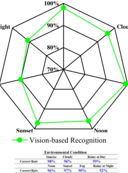
Figure 8 is the vehicle detection results of the proposed system under various weather conditions.

Examples of the detection and segmentation under various whether condition are such as Fig.9. When each vehicle is segmented from the various backgrounds, the vehicles can be continuously processed and counted by the recognition and tracking method during the vehicle appears in the frame. In this period, the experimental environment includes rainy, foggy and various weather condition on different roads. With the proposed method, the average vehicle detection rate is higher than 92%, independent of environmental conditions.

The vehicle recognition rate at night and dim weather condition is lower than the others (that is, sunrise, cloudy, rainy and noon). The suddenly appeared light source (such as headlight, rear light…etc.) causes the outline of vehicle unclear and missed foregrounds and reduces the edge information. But, there is still enough information to detect vehicle by the reflection of rear light.

Table 3 is the accurate rate of the recognition in the heavy traffic (0700~0800 25/01/2007). The recognition rate of 98% was obtained by applying the system to 852 vehicles, only 2% errors occur in the recognition.

In the Fig.10, the proposed system compared with the vision–based vehicle recognition, tracking method and police laser gun (Stalker LIDAR), the vehicle velocity tracking error is not over ±5 km/hr and obtained by applying the system to 30 vehicles.

If we consider the error of the police laser gun, this result should be more accurate.

In Table 4, three separated frames of each model of vehicles are used to demonstrate the superiority of the vehicle recognition method. We can find that the roof, length, and width of different models are quit different. Although the position of a vehicle will change, the visual length of the roof is very close to the roof length of the vehicle no matter where the vehicle is.

Figure 11 is the experimental output of the vehicle recognition and tracking system. In the output, the system can show the traffic parameters of each lane and the total count of each model ― sedans, utility vehicles, vans, mini truck, and large vehicles.

8 Conclusions

In this work, a real time vision-based system to recognize vehicles from image sequences is proposed. The system uses a moving object

detection method to detect the moving vehicles. The system proposes a method to detect and segment the occlusive vehicles. Even though the occlusive vehicles appearing in the images has been keeping merging or having more than two vehicles to merge together all the time, our system can still exactly segment the vehicles. Then, the recognition and tracking methods are proposed to recognize and track the vehicles. This system overcomes various issues raised by the complexity of the outlines of vehicles. Experimental results obtained with the road images reveal that the proposed system can successfully recognize from various vehicles. So far, the system only uses the parameters of the visual length, visual width, and roof to recognize the vehicles. In the future work, more outline features of the vehicles will be considered to increase the recognition rate.

Acknowledgements

Acknowledgment of financial support: Great thanks to Institute of Transportation by the Grant of MOTC-IOT-96-IBB008.

References

[1] J. B. Kim, C. W. Lee, K. M. Lee, T. S. Yun, and H. J. Kim, “Wavelet-based Vehicle Tracking for Automatic Traffic Surveillance,” Proceedings of IEEE Region 10 International Conference on Electrical and Electronic Technology, Vol.1, pp.313-316, 2001.

[2] G. L. Foresti, V. Murino, and C. Regazzoni,

“Vehicle Recognition and Tracking from Road Image Sequences,” IEEE Transactions on Vehicular Technolopy, Vol.48, No.1, 1999.

[3] Y. K. Jung, K. W. Lee, and Y. S. Ho, “Content- Based Event Retrieval Using Semantic Scene Interpretation for Automated Traffic Surveillance,” IEEE Transactions on Intelligent Transportation Systems, Vol.2, No.3, pp.151- 163, 2001.

[4] Z. He, J. Liu, and P. Li, “New method of background update for video-based vehicle detection,” The 7th International IEEE Conference on Intelligent Transportation Systems, pp.580-584, 2004.

[5] C. Stauffer and W. Grimson, “Learning Patterns of Activity Using Real-Time Tracking,” IEEE Transactions on Pattern Analysis and Machine Intelligence, vol.22, pp.747–757, 2000.

[6] I. Haritaoglu, D. Harwood, and L. Davis, “ W⁴: Real-time Surveillance of People and Their Activities,” IEEE Transactions on Pattern Analysis and Machine Intelligence, vol.22, pp.809–830, 2000.

(8)

[7] C. Wren, A. Azarbaygaui, T. Darrell, and A.

Pentland, “Pfinder: Real-Time Tracking of the Human Body,” IEEE Transactions on Pattern Analysis and Machine Intelligence, vol.19, pp.780–785, 1997.

[8] L. Li and M. Leung, “Integrating Intensity and Texture Differences for Robust Change Detection,” IEEE Transactions on Image Processing, vol.11, pp.105–112, 2002.

[9] O. Javed, K. Shafique, and M. Shah, “A Hierarchical Approach to Robust Background Subtraction Using Color and Gradient Information,” IEEE Proceedings of Workshop Motion Video Computing, pp.22–27, 2002.

[10]N. Paragios and V. Ramesh, “A MRF-based Approach for Real-Time Subway Monitoring,”

IEEE International Conference on Computer Vision and Pattern Recognition, vol.1, pp.1034–

1040, 2001.

[11] C. J. Chen, C. C. Chiu, B. F. Wu, S. P. Lin, and C.D. Huang, “The Moving Object Segmentation Approach to Vehicle Extraction,” IEEE International Conference on Networking, Sensing and Control, vol.1, pp.19-23, 2004.

[12]C. C. C. Pang, W. W. L. Lam, and N. H. C.

Yung, “A Novel Method for Resolving Vehicle Occlusion in a Monocular Traffic-Image Sequence,” IEEE Trans. on Intelligent

Transportation Systems, Vol.5, No.3, pp.129- 141, 2004.

[13]X. Song, and R. Nevatia, ”A Model-Based Vehicle Segmentation Method for Tracking,”

Tenth IEEE International Conference on Computer Vision, Vol.2, pp.1124-1131, 2005.

[14]X. Limin, “Vehicle Shape recovery and Recognition Using Generic Models,”

Proceedings of the 4th World Congress on Intelligent Control and Automation, pp.1055- 1059, 2002.

[15]W. Wei, Q. Zhang, and M. Wang, “A method of vehicle classification using models and neural networks,” IEEE VTS 53rd Vehicular Technology Conference, Vol.4, pp.3022-3026, 2001.

[16]N. Ranganathan, R. Mehrotra, and S.

Subramanian, “A high speed systolic architecture for labeling connected components in an image,” IEEE Transactions on Systems, Man and Cybernetics, Vol.25, No.3 , pp.415- 423,1995.

[17]J. Canny, “Finding Edges and Lines in Images,”

M.I.T Artificial Intelligence Laboratory, 1983.

[18]J. R. Parker, “Algorithms for Image Processing and Computer Vision,” Wiley Computer Publishing, pp. 19-53, 1997.

Original Image

Moving Object Segmentation

Input Recognition & Tracking

Occlusion

Occlusive Vehicle Segmentation

Output Vehicle Style

Vehicle Recognition

Vehicle Tracking

Velocity Count

Yes

No

Original Image

Moving Object Segmentation

Input Recognition & Tracking

Occlusion

Occlusive Vehicle Segmentation

Output Vehicle Style

Vehicle Recognition

Vehicle Tracking

Velocity Count

Yes

No

Fig.1 The flowchart of the proposed system

(9)

D₃

D_h2 D₁ D_h1

D₄ H

f

R _p: CCD Vertical Length / Vertical Pixels

F

D₂ θ

Charge-Coupled Device

R₄×R_p R₃×R_p

R₁×R_p R₂×R_p

D₃

D_h2 D₁ D_h1

D₄ H

f

R _p: CCD Vertical Length / Vertical Pixels

F

D₂ θ

Charge-Coupled Device

R₄×R_p R₃×R_p

R₁×R_p R₂×R_p

Fig. 2 The optical geometry (length) between the image and the ground

H

F θ

Dh1 Rw

Dw1 f

CCD

Dh2 H Dw2

F θ

Dh1 Rw

Dw1 f

CCD

Dh2 Dw2

Fig. 3 The optical geometry (width) between the image and the ground

Table 1 The average visual length and visual width of different vehicles

(10)

A B

C D

E The moving object

The moving object’s horizontal edge within the bounding box

The quantification of the horizontal histogram projection:

A to B: the length of the roof B to C: the length of the rear window C to D: the length of the boot

A B

C D

E The moving object

The moving object’s horizontal edge within the bounding box

The quantification of the horizontal histogram projection:

A to B: the length of the roof B to C: the length of the rear window C to D: the length of the boot

(a) Original image (b) The definitions of the horizontal line Fig.4 The outline definitions of a vehicle

Table 2 The measurements of different vehicles

(a) The input image. (b) The foreground image. (c) The occlusion image.

(d) The labeling image after

moving object segmentation. (e) The labeling image after the

occlusion segmentation. (f) Segmented vehicles.

Fig.5 Occlusive segmentation processes

(11)

Fig.6 The location of the stationary video camera Fig.6 The location of the stationary CCD camera

Date: 00:00~12:00 25/01/2007 Location: the Wu-Ling interchange of NO.68 expressway in Hsinchu, Taiwan

0 100 200 300 400 500 600 700 800 900 1000

0~1 1~2 2~3 3~4 4~5 5~6 6~7 7~8 8~9 9~10 10~11 11~12

Time

Vehicle(s)

50%

55%

60%

65%

70%

75%

80%

85%

90%

95%

100%

Counting by System Counting by Hand Correct Rate

Fig.7 The vehicle detection results for the continuous 24 hours

Date: 12:00~00:00 24/01/2007 Location: the Wu-Ling interchange of NO.68 expressway in Hsinchu, Taiwan

0 100 200 300 400 500

12~13 13~14 14~15 15~16 16~17 17~18 18~19 19~20 20~21 21~22 22~23 23~00 Time

Vehicle(s)

50%

55%

60%

65%

70%

75%

80%

85%

90%

95%

100%

Counting by System Counting by Hand Correct Rate

N 24

°

49'34",E 120

°

58'13" the Wu-Ling interchange of NO.68 expressway in Hsinchu, Taiwan ~2006,11,02~

(12)

70%

80%

90%

100%

Sunrise

Cloudy

Rainy at Day

Noon Sunset

Fog Rainy at Night

Vision-based Recognition

Fig.8 The vehicle detection results for various weather conditions

Table 3 Results for different vehicle in the heavy traffic

(13)

At Day

Frame N Frame N+2 Frame N+6 Frame N+8

Rainy at day

At afternoon

Cloudy

At Night

Rainy at night

Fog at night

Fig.9 Examples of the detection and segmentation under various whether condition

(14)

Da t e : 2006.11.08~2006.11.25 Loc a t ion: the Wu-Ling interchange of NO.68 expressway in Hsinchu, Taiwan

60 70 80 90 100

Sample Vehicle'S NO.

Velocity(km/hr)

Vision-Based 80 87 81 72 84 95 96 96 80 74 95 77 90 86 82 78 96 86 77 85 66 75 83 77 69 81 79 78 70 75 Stalker LIDAR 82 87 77 72 85 99 97 98 83 77 99 77 95 89 83 78 99 87 81 89 66 79 83 81 73 81 84 81 74 79 1 2 3 4 5 6 7 8 9 10 11 12 13 14 15 16 17 18 19 20 21 22 23 24 25 26 27 28 29 30

Fig.10 Results of the vehicle velocity

Table 4 The visual length, width, and roof of the vehicles in a frame sequence (H=6 m, θ=14°, f=8 mm, Rp=0.025 mm/pixel)

(15)

Fig.11 The display of the system