以矩陣分解法計算特別階段形機率分配並有多人服務之排隊模型 - 政大學術集成
77
0
0
全文
(2) Abstract Stationary probabilities are fundamental in response to various measures of performance in queueing networks. Solving stationary probabilities in Quasi-Birth-and-Death (QBD) with phase-type distribution normally are dependent on the structure of the queueing network. In this thesis, a new computing scheme is developed for attaining stationary probabilities in queueing networks with multiple servers. This scheme provides a general approach of considering the complexity of computing algorithm. The result becomes more significant when a large matrix is involved in. 政 治 大 departure process and the moments of inter-departure times. We com立. computation. After determining the stationary probability, we study the. pute the moments of inter-departure times and the variance by applying. ‧ 國. 學. two numerical methods (Matlab and Promodel). The lagk correlation of inter-departure times is also introduced in the thesis. The proposed. ‧. approach is proved theoretically and verified with illustrative examples.. n. er. io. sit. y. Nat. al. Ch. engchi. i. i n U. v.
(3) 中文摘要 穩定狀態機率是讓我們了解各種排隊網絡性能的基礎。在 擬生死過程 (Quasi-Birth-and-Death) Phase-type 分配中求得穩定狀態機率,通常是依賴排隊 網絡的結構。在這篇論文中,我們提出了一種計算方法-LU 分解,可以求得在排 隊網絡中有多台服務器的穩定狀態機率。此計算方法提供了一種通用的方法,使 得複雜的大矩陣變成小矩陣,並減低計算的複雜性。當需要計算一個複雜的大矩 陣,這個成果變得更加重要。文末,我們提到了離開時間間隔,並用兩種方法 (Matlab 和 Promodel) 去計算期望值和變異數,我們發現兩種方法算出的數據相. 治 政 近,接著計算離開顧客的時間間隔相關係數。最後,我們提供數值實驗以計算不 大 立 同服務器個數產生的離去過程和相關係數,用來說明我們的方法。 ‧. ‧ 國. 學. n. er. io. sit. y. Nat. al. Ch. engchi. ii. i n U. v.
(4) 誌謝 在學校教書多年,來到政大應數系接觸等候理論,承蒙恩師 陸行教授認真 的指導,在研究所三年的學習階段,多次的討論過程中獲益良多,在此致上最衷 心的謝意和敬意。口試期間,承蒙 張國華教授、曾正男教授不吝惠賜諸多寶貴 意見,使得本論文更趨完整,特此銘謝。 研究期間,首先感謝王嘉宏學長對論文結構、寫法的指導,更要感謝林隽民 同學在數學運算程式的寫法、運算過程的指導,在經過不斷的嘗試與挫折中,最. 政 治 大. 後得到正確的數據,猶如荒漠之中遇見桃花源。也感謝學弟們,在每次討論之中,. 立. 讓我得到許多啟發。. ‧ 國. 學. 這段期間所面臨的壓力,感謝我的同事,不時的關心與鼓勵。以及我親愛的. ‧. 老婆珮璇,每天細心呵護我的健康,給我滿滿的愛。最後衷心感謝我的父母對我 的栽培,因為有你們背後的支持,得以順利完成碩士學位,願將此項殊榮獻給我. y. Nat. n. al. er. io. sit. 最摯愛的家人共享。. Ch. engchi. ii. i n U. v.
(5) Contents Abstract . . . . . . . . . . . . . . . . . . . . . . . . . . . . . . . . . . . . .. i. Abstract in Chinese . . . . . . . . . . . . . . . . . . . . . . . . . . . . . . .. ii. Acknowledgment. 政 治 大 . . . . . . . . . . . . . . . . . . . . . . . . . . . . . . . . 立. iii. Nat. 4. y. 2 Problem Definitions. 4. 2.2. A phase-type queueing model . . . . . . . . . . . . . . . . . . . . . .. n. er. sit. Markovian arrival process with phase-type distributions . . . . . . . .. io. 2.1. al. Ch. 3 Matrix-Geometric Solutions. engchi. i n U. 1. ‧. ‧ 國. 學. 1 Introduction. 7. v. 12. 3.1. State balance equations . . . . . . . . . . . . . . . . . . . . . . . . . . 12. 3.2. An algorithm for matrix decomposition . . . . . . . . . . . . . . . . . 14. 4 Inter-Departure times. 23. 4.1. Departure process . . . . . . . . . . . . . . . . . . . . . . . . . . . . . 23. 4.2. Moments of inter-departure times . . . . . . . . . . . . . . . . . . . . 25. 4.3. Lagk correlations between successive departures . . . . . . . . . . . . 25. iv.
(6) 5 Numerical Examples. 27. 5.1. Queueing models with two servers . . . . . . . . . . . . . . . . . . . . 27. 5.2. Queueing models with three servers . . . . . . . . . . . . . . . . . . . 37. 5.3. Queueing models with more than twenty servers . . . . . . . . . . . . 46. 5.4. Numerical experiments with more than forty servers . . . . . . . . . . 55. 6 Conclusion. 59. Appendix A. 立. Appendix B. 64. ‧ 國. 65. ‧ 68. n. al. er. io. sit. y. Nat. Appendix D. 62. 學. Appendix C. 政 治 大. Ch. engchi. v. i n U. v.
(7) List of Figures 2.1. A semi M AP/M/n queueing model . . . . . . . . . . . . . . . . . . .. 5.1. The queue empty rate determined by four different methods . . . . . 51. 5.2. Relative errors of three methods compared with Promodel . . . . . . 52. 5.3. The queue empty rate determined by four different methods . . . . . 53. 5.4. Relative errors of three methods compared with Promodel . . . . . . 53. 5.5. The queue empty rate determined by four different methods . . . . . 54. 5.6. Relative errors of three methods compared with Promodel . . . . . . 54. 5.7. Condition number determined by Q3 . . . . . . . . . . . . . . . . . . 56. 5.8. Condition number determined by P1 . . . . . . . . . . . . . . . . . . 57. 5.9. The queue empty rate computed by LU method . . . . . . . . . . . . 57. 立. 5. 政 治 大. ‧. ‧ 國. 學. n. er. io. sit. y. Nat. al. Ch. engchi. i n U. v. 5.10 The queue empty rate computed by RA method . . . . . . . . . . . . 58. vi.
(8) List of Tables 5.1. Arrival processes of two phases simulated in Promodel. . . . . . . . . 29. 5.2. 政 治 大 Probabilities obtained from three methods with p = 0.4, 0.5, 0.6. 立. 5.3. Probabilities obtained from three methods with p = 0.1, 0.2, 0.3. . . 31 . . 32. Comparison of queue empty rates of two servers. . . . . . . . . . . . . 32. 5.5. Probabilities obtained from three methods with p = 0.2, 0.3, 0.4. . . 39. 5.6. Probabilities obtained from three methods with p = 0.5, 0.6, 0.7. . . 40. 5.7. Probabilities obtained from three methods with p = 0.8, 0.9. . . . . . 41. 5.8. Comparison of the queue empty rates of three servers. . . . . . . . . . 42. 5.9. . . . . 48. ‧. ‧ 國. 學. 5.4. er. io. sit. y. Nat. al. n. v i n C U probabilities p. The queue empty rate ofhtwenty e n gservers c h iversus. 5.10 The queue empty rate of twenty-five servers versus probabilities p. . . 49 5.11 The queue empty rate of thirty servers versus probabilities p. . . . . . 51 5.12 Comparison of queue empty rates of twenty servers. . . . . . . . . . . 51 5.13 Comparison of queue empty rates of twenty-five servers. . . . . . . . . 52 5.14 Comparison of queue empty rates of thirty servers. . . . . . . . . . . 53. vii.
(9) Chapter 1 Introduction. 立. 政 治 大. The Markovian arrival process (MAP) is a generalization of the Poisson process, We consider a semi. ‧ 國. 學. where the arrivals are governed by a Markov chain [10].. M AP/M/n queueing system, where customers arrive at the system according to. ‧. a phase-type process but may leave the system without services. The family of phase-type distributions is widely used in algorithmic probability [5]. A continu-. y. Nat. sit. ous time phase-type distribution is the distribution of the time until absorption in. er. io. an absorbing Markovian process. We assume the inter-arrival time follows a typ-. al. v i n the system are identical, and C their service times are h e n g c h i U independent and identically distributed (i.i.d.) random variables following exponential distributions. Each inn. ical MAP but the arrival rate is smaller since the renege occurs. All n servers of. coming customer receives service immediately if he/she finds an idle server upon arrival. Although M AP/M/n queues have been studied extensively by many researchers, analytical solutions for the stationary probability have not yet been studied comprehensively in the literature [5]. In this thesis, we study the stationary distribution of such a semi M AP/M/n queueing system with multiple servers. We compute the stationary probability by applying the matrix geometric solution procedure in [8], which will be combined with Ramaswami’s formula [7] and block LU factorization [6] in this thesis. The main contribution in the thesis is to present a matrix decompo-. 1.
(10) sition approach for the stationary probability in a phase-type M AP/M/n queueing model. Through solving the system of sub-matrices by using Matrix-Geometric Solution Method, we obtain the stationary probability. Matrix analytic methods are popular as modeling tools because they give one the ability to construct and analyze a wide class of queueing models in a unified and algorithmically tractable way [7]. The Matrix-Geometric Solution Method [5, 8] relies on identifying two parts within the structure of the underlying continuous time Markov chain, including the initial/boundary part and the repetitive part. The initial part has a non-regular structure and each component in it must be represented in detail [8]. The repetitive part has a regular structure and can be represented in. 政 治 大. stochastic process algebras as a composition of several components. In Matrix-. 立. Geometric Solution Method, the infinitesimal generator matrix is decomposed into. ‧ 國. 學. sub-matrices, with each one of them representing the transition rates in a particular area within a given part, or between them [5, 8]. The size of the state space would. the Markovian process even if the system is infinite [3].. Nat. y. ‧. be reasonably small compared with the size of the infinitesimal generator matrix of. sit. The inter-departure times of customers leaving the system are correlated [4].. er. io. In the standard network node approximation approach, the departure process from a. al. n. v i n C h distributed (i.i.d.). times are independent and identically e n g c h i U However, this i.i.d.. workstation system is normally approximated by assuming that these inter-departure as-. sumption allows for a simple approximation [12] of the squared coefficient of variation (SCV) of departure process (Cd2 ) as a function of the systems utilization (u) and the arrival and service processes SCV’s (Ca2 , Cs2 ) for a G/G/n queue as √ Cd2 = (1 − u2 )(Ca2 − 1) + u2 (Cs2 − 1)/ n.. Bitran and Dasu [1] developed a phase-type distribution representation of the departure process from a single server system and provided moments of the interP departure times of a P hi /P h/1 queue. We extend those results to get the moment of inter-departure times and correlations between successive departures.. 2.
(11) The remainder of the thesis is organized as follows. Chapter 2 introduces a queueing model with phase-type Markovian arrival process. In Chapter 3, we present a matrix decomposition approach for the stationary probability in a phase-type M AP/M/n queueing model by applying the Matrix-Geometric Solution Method combined with Ramaswami’s formula and LU factorization. We introduce the interdeparture times in Chapter 4. Numerical results of M AP/M/n queueing systems with multiple servers are given in Chapter 5, and numerical results of the stationary distribution are compared with approximation methods and simulations. Concluding remarks are to be given in Chapter 6.. 立. 政 治 大. ‧. ‧ 國. 學. n. er. io. sit. y. Nat. al. Ch. engchi. 3. i n U. v.
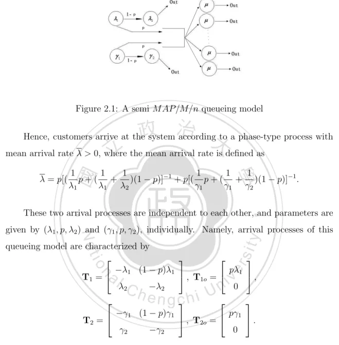
(12) Chapter 2 Problem Definitions. 立. Markovian arrival process with phase-type dis-. 學. ‧ 國. 2.1. 政 治 大. tributions. ‧. We consider a single queueing station and model the queueing network as a semi. y. Nat. sit. M AP/M/n queue shown in Fig. 2.1, where n servers are all identical. The mean. al. er. io. service times of each server is exponentially distributed with rate µ. Let S1 and S1o. v. n. represent a transition of service that customer stays with the server and finishes the service, individually, i.e.,. Ch. S1 =. h. e ni g c h ih. −µ. , S1o =. i n U. µ. i. .. The queueing network has two independent and identical arrival streams, where there are two phases for each arrival stream [4]. For the first arrival stream, the time spent in the first phase is exponentially distributed with rate λ1 , and the time spent in the second phase is also exponentially distributed with rate λ2 . Similarly, for the other arrival stream, the time spent in the first phase is exponentially distributed with rate γ1 , and the time spent in the second phase is also exponentially distributed with rate γ2 . After the first phase of arrival stream, the incoming arrival goes to the queueing system (and is to be served) with probability 0 ≤ p ≤ 1; otherwise, it. 4.
(13) jumps to the second phase and then departs directly with probability (1 − p). All arrival streams operate in a similar manner.. Figure 2.1: A semi M AP/M/n queueing model. 政 治 大. Hence, customers arrive at the system according to a phase-type process with. 立. mean arrival rate λ > 0, where the mean arrival rate is defined as 1 1 1 1 1 1 p + ( + )(1 − p)]−1 + p[( p + ( + )(1 − p)]−1 . λ1 λ1 λ2 γ1 γ1 γ2. ‧. ‧ 國. 學. λ = p[(. These two arrival processes are independent to each other, and parameters are. y. Nat. given by (λ1 , p, λ2 ) and (γ1 , p, γ2 ), individually. Namely, arrival processes of this. sit. n. al. er. io. queueing model are characterized by −λ1 (1 − p)λ1 pλ , T1o = 1 , T1 = λ2 −λ2 0 T2 = . Ch. e n g c h i. −γ1 (1 − p)γ1 γ2. −γ2. i n U . , T2o = . v. pγ1 0. .. Note that matrices Tm , for m = 1, 2 correspond to phase transitions, and Tmo corresponds to the rate as arrivals enter the system. Both arrival processes are MAP distributed inter-arrival times denoted by (e1 , Tm , Tmo ), for m = 1, 2, where e1 is a 2 × 1 vector with the first element equals to 1 and another element equals to 0. The advantage of phase-type distributions is their generality and versatility, which permits the calculation of performance measures of stochastic models with a high degree of accuracy [3]. The Matrix-Geometric Solution Methods allows us to. 5.
(14) deal with the models whose activities are not necessarily exponentially distributed, while at the same time overcoming the problem of the rapid growth of the state space introduced by the need to explicitly construct the infinitesimal generator matrix of the underlying Markovian process. The one-step transition matrix embedded in the Markov chain of the arrival process is given by . B C 0 0 ··· 00 0 B00 C 0 · · · Φ= 0 0 B00 C · · · .. .. .. .. . . . . . . .. , . (2.1). 政 治 大 where there exists nonnegative off-diagonal and negative diagonal elements in the 立. ‧ 國. is the infinitesimal generator of the MAP, we have. ‧. (B00 + C)1 = 0,. 學. matrix B00 = [bij ], and the elements of matrix C = [cij ] are nonnegative. Since Φ. sit. y. Nat. where 1 is an 4 × 1 vector with all its elements equal to 1. Since (B00 + C) is the infinitesimal generator, there exists a stationary probability vector. n. where θ i,j. er. io. a l θ = (θ , θ , θ , θ ), i v n Ch U i is in the i-th phase of the first e nthatg an c harrival is the stationary probability 1,1. 1,2. 2,1. 2,2. stream and the other arrival is in the j-th phase of the second stream. The repetition of the state transitions for vector processes implies a geometric form where scalars are replaced by matrices. Such Markovian processes are called Matrix-Geometric Solution processes. To determine the stationary probability, we need to solve the following balance equations θ(B00 + C) = 0, θ1 = 1.. In the following section, we recall a special phase-type distributions.. 6.
(15) 2.2. A phase-type queueing model. In general, the embedded Markov chain is ergodic if the stability condition of the system is ρ = λ/(nµ) < 1. Lemma 1. Given the mean arrival rate λ > 0 and ρ = λ/(nµ) < 1, the effective range of p is 0 6 p < w, where w = min{1,. −b −. √. b2 − 4ac }, 2a. a = γ1 γ2 λ1 + λ1 λ2 γ1 + nµλ1 γ1 ,. 政 治 大. b = −(λ1 λ2 γ2 + γ1 γ2 λ1 + λ1 λ2 γ1 + γ1 γ2 λ2 + nµλ2 γ1 + 2nµλ1 γ1 + nµλ1 γ2 ), and. 立c = nµ(λ + λ )(γ + γ ). 1. 1. 2. ‧. ‧ 國. 學. Proof :. 2. Because λ/(nµ) < 1, we have. 1 1 1 1 1 1 p + ( + )(1 − p)]−1 + p[( p + ( + )(1 − p)]−1 < nµ. λ1 λ1 λ2 γ1 γ1 γ2. sit. (2.2). n. al. er. io. It implies that. y. Nat. λ = p[(. Ch. i n U. v. λ1 p γ1 p + < nµ. λ1 + λ2 − λ1 p γ1 + γ2 − γ1 p. engchi. (2.3). By using the form ap2 + bp + c > 0, we can combine the above inequality, and then solve the inequality. It gives p>. −b +. or p<. −b −. √. b2 − 4ac , 2a. √. b2 − 4ac , 2a. where a = γ1 γ2 λ1 + λ1 λ2 γ1 + nµλ1 γ1 , b = −(λ1 λ2 γ2 + γ1 γ2 λ1 + λ1 λ2 γ1 + γ1 γ2 λ2 + nµλ2 γ1 + 2nµλ1 γ1 + nµλ1 γ2 ),. 7.
(16) and c = nµ(λ1 + λ2 )(γ1 + γ2 ). Because the probability p satisfies 0 6 p 6 1, we have 0 6 p < w if √ −b − b2 − 4ac }. w = min{1, 2a Let A(t) denote the number of customers arriving in (0, t] and J(t) be the state of the Markov chain at time t with state space {(1, 1), (1, 2), (2, 1), (2, 2)}. Then {A(t), J(t)} is a three-dimensional Markovian process with state space {(k, i, j) : k ≥ 0, i, j = 1, 2}, where k is the number of customers in the system, i is the phase of the first arrival stream, and j is the phase of the second arrival stream.. 政 治 大 for k > 0. Then, there exists an integer n such that the levels 0 up to n − 1 from 立 The state {(k, 1, 1), (k, 1, 2), (k, 2, 1), (k, 2, 2)} is called the level k of the system,. ‧ 國. 學. the boundary, and those for k > n are repeating. Transitions between the repeating states have the property that the rates from (k, i, j) to the state (k + v, i0 , j 0 ) for 0 6 v 6 ∞ and i0 , j 0 = 1, 2 are independent of the value k for k > n. From that n. ‧. onwards, the behavior of the system for all k > n is the same as the behavior of the. sit. y. Nat. system for n, where k is the number of queued customers. Such similarity needs not. io. in the system as. n. al. πk =. er. for (0, 1, · · · , n − 1). We define the vector of probabilities that there are k customers. v i n lim P r{A(t) = k, J(t) = (i, j)} C hengchi U. t→∞. = (πk,1,1 πk,1,2 πk,2,1 πk,2,2 ),. (2.4). where π can be partitioned into blocks which correspond to state 0, state 1, state 2, etc., e.g., π = (π 0 , π 1 , π 2 , · · · ). Recall that the Kronecker product of any two matrices L and M is defined as L ⊗ M = [lij M] f or all i, j, where lij is the ith row and jth column element of the matrix L. In addition, the Kronecker sum of any two matrices L and M is given by L ⊕ M = L ⊗ IM + IL ⊗ M.. 8.
(17) By applying Kronecker matrix operations, we obtain −λ1 − γ1 (1 − p)γ1 (1 − p)λ1 0 γ2 −λ1 − γ2 0 (1 − p)λ1 B00 = T1 ⊕ T2 = λ2 0 −λ2 − γ1 (1 − p)γ1 0 λ2 γ2 −λ2 − γ2 and. C = (T1o ⊗ eT1 ) ⊕ (T2o. p(λ1 + γ1 ). 0. 0. 0. pλ1. 0. 0. 0. pγ1. 0. 0. 0. T ⊗ e1 ) = . 0. , . . 0 . 0 0. 政 治 大. Using the arrival and service process parameters in terms of the Kronecker. 立. product and sum, we obtain sub-matrices A10 , A21 , A(i)(i−1) , A, which represent a. ‧. ‧ 國. 學. customer is in service, finishes the service, and departs the system, respectively. µ 0 0 0 0 µ 0 0 , A10 = IT ⊗ S1o = 0 0 µ 0 0 0 0 µ 2µ 0 0 0 0 2µ 0 0 , A21 = IT ⊗ (S1o ⊕ S1o ) = 0 0 2µ 0 0 0 0 2µ iµ 0 0 0 0 iµ 0 0 , A(i)(i−1) = IT ⊗ (S1o ⊕ · · · ⊕ S1o ) = | {z } 0 0 iµ 0 i 0 0 0 i)µ. n. er. io. sit. y. Nat. al. Ch. engchi. i n U. v. for 3 6 i 6 n − 1 and . nµ 0 0 0 0 nµ 0 0 A = IT ⊗ (S1o ⊕ · · · ⊕ S1o ) = {z } | 0 0 nµ 0 n 0 0 0 nµ. 9. , .
(18) where IT is an identity matrix of dimensions equal to the sum of the dimensions of the two arrival processes, i.e., IT = I4×4 . Next, we define sub-matrices B00 , B11 , Bii , and B as follows, where the internal phase changes for the composite arrival process, which are B00 = T1 ⊕ T2 . −λ1 − γ1 (1 − p)γ1 (1 − p)λ1. = . γ2. −λ1 − γ2. 0. λ2. 0. −λ2 − γ1. 0. λ2. γ2. . 0. (1 − p)λ1 , (1 − p)γ1 −λ2 − γ2. 政 治 大. B11 = T1 ⊕ T2 ⊕ S1 −λ1 − γ1 − µ (1 − p)γ1 (1 − p)λ1 0 γ2 −λ1 − γ2 − µ 0 (1 − p)λ1 = λ2 0 −λ2 − γ1 − µ (1 − p)γ1 0 λ2 γ2 −λ2 − γ2 − µ. 立. ‧. ‧ 國. 學. −λ1 − γ1 − iµ. al. n. = . γ2. y. (1 − p)γ1. (1 − p)λ1. Ch. −λ1 − γ2 − iµ. v ni. 0. c h−i γU− iµ 0 e n g −λ. λ2. 2. 0. , . sit. io. . i. er. Nat. Bii = T1 ⊕ T2 ⊕ S1 ⊕ · · · ⊕ S1 | {z }. . λ2. 1. γ2. 0 (1 − p)λ1 (1 − p)γ1. −λ2 − γ2 − iµ. , . for 2 6 i 6 n − 1, B = T 1 ⊕ T 2 ⊕ S1 ⊕ · · · ⊕ S1 | {z } n. = . −λ1 − γ1 − nµ. (1 − p)γ1. (1 − p)λ1. 0. γ2. −λ1 − γ2 − nµ. 0. (1 − p)λ1. λ2. 0. −λ2 − γ1 − nµ. (1 − p)γ1. 0. λ2. γ2. −λ2 − γ2 − nµ. 10. , .
(19) and. C = (T1o ⊗ eT1 ) ⊕ (T2o. p(λ1 + γ1 ). T ⊗ e1 ) = . 0. 0. 0. pλ1. 0. 0. 0. pγ1. 0. 0. 0. 0. . 0 0 0. representing that a customer goes into the queueing system. Hence, in our queueing model, there exists the infinitesimal generator matrix of a continuous time Markovian process with the structure,. 立. A10 B11. A21 B22 .. .. . .. .... 0 .. .. ... .. . B(n−1)(n−1). 0. 0. ... 0. 0. 0. .... 0 .. .. 0 .. .. 0 .. .. Nat. 0. ... A. .. 0 .. .. .. .. ···. 0. ··· 0 0 ··· .. .. .. . . . , C 0 ··· B C ··· A B ··· .. .. .. . . . 0. (2.5). ‧. ‧ 國. 0 .. .. ··· 0 0 治 政 ... 大0 0 C 0. y. C. io. sit. B00. . 學. Q= . er. . where n is the number of servers in the system. The matrix Q is composed of. n. al. Ch. i n U. sub-matrices along with the block tridiagonal matrix.. engchi. 11. v.
(20) Chapter 3 Matrix-Geometric Solutions. 立. State balance equations. 學. ‧ 國. 3.1. 政 治 大. The stationary probabilities for the queue satisfy πQ = 0, π1 = 1, and π > 0. We. ‧. n. Ch. U i e h n c g π C + π B + π A = 0, 1. 2. 22. 3. sit. io. al. π 0 C + π 1 B11 + π 2 A21 = 0,. er. Nat. π 0 B00 + π 1 A10 = 0,. y. can find the π i ’s by solving the following state balance equations (3.1)-(3.5):. v ni. 32. (3.1). (3.2). (3.3). .. . π n−2 C + π n−1 B(n−1)(n−1) + π n A(n)(n−1) = 0.. (3.4). The equation for the repeating states of the process is given by: π i−1 C + π i B + π i+1 A = 0, i = n, n + 1, n + 2, · · · .. (3.5). Using (3.5), the matrix geometric procedure gives the vector solution π n+k−1 = π n−1 Rk , for k = 0, 1, 2, · · · , where R is the matrix solution of the equation C +. 12.
(21) RB + R2 A = 0. Neuts [8] showed that the iteration Rk+1 = −(C + R2k A)B−1 converges to the solution R starting with R0 = 0. We rewrite the above equations (3.1)-(3.5) in matrix form as follows h. π0 π1 · · ·. π n−1 π n. i. · Q1 = 0,. (3.6). where . B00. C. 0. ···. 0. 0. . 0. A10 B11 C 0 ··· 0 0 0 A21 B22 C ··· 0 0 Q1 = .. .. .. .. .. .. .. . . . . . . . 0 0 0 · · · A(n−1)(n−2) B(n−1)(n−1) C 0 0 0 ··· ··· A B + RA. 立. 政 治 大. ‧. ‧ 國. 學. . . In addition, by using the normalization condition, we obtain. Nat. y. π 0 · 1 + π 1 · 1 + · · · + π n (I − R)−1 · 1 = 1.. al. er. io. sit. (3.7). n. Then the solution for the probabilities π 0 , π 1 ..., π n can be determined by h. Ch. π0 π1 · · ·. i. eπn g cπ h i n−1. n. iv n U = [1, 0], ·Q. (3.8). 2. where Q2 = . C. 0. ···. 0. 0. C. ··· .. . .... 0. 0. 0 .... 0 .... 1. B00. 1. A10 B11. 1 .. .. 0 .... 1. 0. 0. ···. (I − R)−1 · 1. 0. 0. ···. A21 B22 ... .... A(n−1)(n−2) B(n−1)(n−1) ···. A. C B + RA. . . By the stability assumption, the infinitesimal generator matrix is irreducible. The necessary condition for this is that matrices B and Bii , for i = 0, 1, 2, · · · , n − 1,. 13.
(22) are nonsingular, which implies that inverses of those matrices can be determined. The computation of the matrix R is by means of the iterative procedure [5]. The sequence {Rk }k is entry-wise nondecreasing and converges monotonically to a nonnegative matrix R. This follows the fact that B−1 is a nonnegative matrix. The number of iterations needed for convergence increases as the spectral radius of R increases. We terminate the iteration and return with the solution of R when kRk+1 − Rk k∞ 6 ε, where ε is a given small constants.. An algorithm 立 for matrix decomposition. 學. ‧ 國. 3.2. 政 治 大. Ramaswami’s formula [7]. n. al. ···. . ··· = 0, ··· .... er. io. sit. y. ‧. Nat. Consider computing π such that πQ = 0. That is, B B1 0 0 0 h i B−1 B C 0 ∗ π π n+1 π n+2 · · · 0 A B C ... ... ... .... Ch. i n U. engchi. v. where π ∗ = [π 0 , π 1 , ..., π n ], B C 0 ··· 0 0 00 .. . A10 B11 C 0 0 ... 0 A21 B22 0 0 B0 = . .. .. .. .. .. , . . . . . . . 0 0 · · · A(n−1)(n−2) B(n−1)(n−1) C 0 0 ··· ··· A B B−1 =. h. 0 ···. 0 A. 14. i 4×4(n+1). ,.
(23) B1 = . . 0 .. . 0 C. .. 4(n+1)×4. It also gives . B C 0 A B C 0 A B .. .. .. . . . where. . V0 V1. ···. . ··· = VW, ··· .. .. 治 I 0 ··· 政 大 −H I ··· . 0. 立. ‧ 國. ,W = 0 .. .. 0 ··· . −H I · · · .. .. .. . . .. . . y. Nat. B B1 0 ··· 0 i B−1 ··· 0 VW .. .. n which is equivalent to. Ch. engchi . π ∗ π n+1 π n+2. As we know I 0 0 H I 0 W−1 = 0 H I ... .. .. . .. ···. = 0, . sit. io. al. er. π ∗ π n+1 π n+2. h. ‧. Then we have. h. . 學. 0 V0 V1 V= 0 0 V0 · · · .. .. .. .. . . . .. ···. 0. B0. i B−1 ··· 0 .. .. i n U. B∗1. v. 0 ···. V. = 0. . . h i h i ··· , and B∗ 0 0 · · · = B 0 0 · · · W−1 . 1 1 ··· .. .. 15.
(24) Then, we have B∗1 = B1 · I. Next, to determine H and V0 , we solve the following equations: V0 − V1 H = B,. V1 = C, and −V0 H = A.. 政 治 大. From the first two equations, it yields h i B0 B1 = 0. π ∗ π n+1 B−1 V0. 立. ‧ 國. 學. π ∗ (B0 − B1 V0−1 B−1 ) = 0. io. sit. y. (3.9). er. Nat. and. ‧. Then, by solving the following equations. π 0 · 1 + π 1 · 1 + · · · + π n (I − R)−1 · 1 = 1,. n. al. we get π ∗ = [π 0 , π 1 , ..., π n ].. Ch. engchi. i n U. v. LU factorization Considering the matrix Q1 . Here, we assume that π ∗ Q1 = 0. The equations are of the homogeneous system. We use LU factorization to obtain π ∗ in the following steps. Step 1: Let the first column of Q1 be replaced by the column vector (1, · · · , 1, (I − R)−1 · 1)T .. 16.
(25) Then, the modified Q1 is rewritten as a new matrix Q3 , and we have π ∗ Q3 =. h. y 0 ···. i. 0. ,. where y=. h. 1 0 0 0. i. .. Step 2: If we transpose π ∗ Q3 , it gives (π ∗ Q3 )T = QT3 π ∗ T. Ω. BT22 A32 · · · .. .. .. . . .. 0 .. .. C. BT(n−1)(n−1). ···. C. ···. 0. 0. io. where. ···. BT00. A10 ∗. ∗. 1 0 = 0 0. al. 1. Ch. y. Nat. 0. π0 π1 0 π2 0 · .. .. . . π n−1 A T πn (B + RA) Ω. 0. 0. 0. . Ω. ···. A21. C .. .. ···. ‧. B11. T. Ω. . er. A10. 政 治 0大. n. C 0 .. . 0 0. ∗. ‧ 國. ∗ BT00. . . 學. . 0 .. .. . sit. 立. Then, we have. y. = . T. n U e n1 g c h i 1. (1 − p)γ1 −λ1 − γ2 = (1 − p)λ1 0 0 (1 − p)λ1 1 1 1 1 1 0 0 µ 0 0 ,Ω = 0 0 0 µ 0 0 0 µ 0 0. . . y. = . iv. 1. 0. λ2. −λ2 − γ1. γ2. T. 0 0 .. . 0 0. , . , . (1 − p)γ1 −λ2 − γ2 (I − R)−1 · 1 1 1 0 0 0 ,Ω = 0 0 0 0 0 0. . . Step 3: Applying Gaussian elimination, we transform Ω and Ω into a zero matrix.. 17.
(26) Then it gives ∗∗ BT A10 ∗∗ 0 0 00 C BT11 A21 0 0 C BT22 A32 Zn = . ... ... ... .. 0 0 0 ··· 0 0 0 ···. ···. 0. 0. ···. 0. 0. ··· .... 0 .... 0 .... C. BT(n−1)(n−1). A. ···. C. (B + RA)T. , . ∗∗. where BT00 , A10 ∗∗ , are obtained by Gaussian elimination. Theorem 1. Zn is a nonsingular matrix.. 政 治 大 Proof : By Step 1, we know 立. y=. h. y 0 ···. 1 0 0 0. 0. i. i. ,. ‧. ‧ 國. π Q3 =. h. 學. where. ∗. .. y. Nat. io. sit. The solution of π ∗ is unique by Matrix Geometric Solution, and Q3 is a non-. n. al. er. sigular matrix. We transpose the matrix Q3 to QT3 . By Step 3, we determine Zn . Q3 is a nonsigular matrix, so is Zn .. Ch. engchi. i n U. v. Theorem 2. (Roger and Charles [9]) Let Z ∈ Mm×m , a set of m × m matrices. There exists permutation matrices D, E ∈ Mm×m , a lower triangular matrix L ∈ Mm×m , and an upper triangular matrix U ∈ Mm×m such that Z = DLUE.. If Z is nonsingular, one may take E = I and Z may be written as Z = DLU.. Proof :. 18.
(27) If rank Z=k, Z has a k-by-k nonsingular submatrix, which may, by permutation of rows and columns, be permuted into the upper left corner. Now apply Theorem D in Appendix B to the upper left corner and apply Theorem LU in Appendix A to achieve a factorization. If Z is nonsingular, Theorem D in Appendix B indicates that permutation on the right is unnecessary in order to apply Theorem D in Appendix B, which verifies the second factorization and completes the proof. Step 4: By . , . 政 治00 大 Z ·π n. ∗T. .. .. 0 0. 學 ‧. ‧ 國. 立. = . yT. and according to above Theorems 1 and 2, we can infer that as follows Remark 1. y. Nat. and Remark 2. Let Zn ({i}), i = 1, · · · , 4(n + 1) be formed with the first i rows. n. al. er. io. · · · , Zn ({i}).. sit. squared matrix of Zn . Zn ({1, 2, · · · , i}) denote a series of matrices Zn ({1}), Zn ({2}),. Ch. i n U. v. Remark 1. Zn is a 4(n + 1) × 4(n + 1) matrix and nonsingular, and. engchi. det(Zn )({1, · · · , j}) 6= 0, ∀ j = 1, · · · , 4(n + 1), which implies Zn = LU [9]. Because Zn = LU, we can slove [π 0 , π 1 , ..., π n ] by T y 0 0 ∗T LU · π = . . .. 0 0. 19.
(28) . It gives the LU factorization of Zn as follows: I 0 0 0 ··· 0 0 U F1 0 0 0 L1 I 0 0 ··· 0 0 0 U1 F2 0 0 L2 I 0 ··· 0 0 0 0 U2 F3 · . .. . . . . . . . . . . . . . . . . . . .. . . . . . . . . . . 0 0 0 · · · Ln−1 I 0 0 0 0 ··· 0 0 0 · · · · · · Ln I 0 0 0 ···. ···. 0. 0. ···. 0. 0. ··· .... 0 .... 0 .... 0 ···. Un−1 Fn 0. Un. . . The following algorithm is given for Li and Ui :. 政 治 大. Algorithm 1: LU factorization. 學. for i = 1 : n. 立. ∗∗. ‧ 國. Input U0 = BT00. ‧. do Li = CU−1 i−1 ∗. sit. io. n. al. er. end. y. Nat. do Ui = BTii − Li Fi. Ch. i n U. v. After completing the LU factorization, the vector π can be obtained via block forward and backward substitution:. engchi. Algorithm 2: Forward and backward substitution Input y0 = [1, 0, 0, 0]T for i = 1 : n do yi = −Li yi−1 end do π n = U−1 n yn. 20.
(29) for i = n − 1 : −1 : 0 do π i = U−1 i (yi − Fi+1 π i+1 ) end. According the above algorithm, we obtain the stationary probability π ∗ = [π 0 , π 1 , ..., π n ]. Remark 2. If Zn is a 4(n + 1) × 4(n + 1) matrix and singular with some 1 ≤ j ≤ 4(n + 1) such that det(Zn )({j}) = 0,. 政 治 大. then by Theorem 2 there exists a permutation matrix D ∈ M4(n+1)×4(n+1) matrix. 立. such that. ‧ 國. 學. det(DT Zn )({1, · · · , j}) 6= 0, j = 1, · · · , 4(n + 1). which implies DT Zn = LU and Zn = DLU.. n. Ch. engchi. y. . sit. yT. 0 0 .. . . 0 0. er. io. al. ‧. Nat. Because Zn = DLU, we can slove π ∗ by yT 0 0 T ∗ T ∗T DLU · π = .. ⇒ LU · π = D · . 0 0. i n U. v. After completing the LU factorization, the vector π can be obtained via block forward and backward substitution:. Algorithm 1: Forward and backward substitution Input y0 = [DT ({4})][1, 0, 0, 0]T for i = 1 : n do yi = −Li yi−1. 21.
(30) end do π n = U−1 n yn for i = n − 1 : −1 : 0 do π i = U−1 i (yi − Fi+1 π i+1 ) end. In the above Algorithm, DT ({4}) is the first four rows and columns composing a 4 × 4 matrix.. 政 治 大. According to the above algorithm, we obtain the stationary probability π ∗ =. 立. [π 0 , π 1 , ..., π n ].. ‧. ‧ 國. 學. n. er. io. sit. y. Nat. al. Ch. engchi. 22. i n U. v.
(31) Chapter 4 Inter-Departure times. 立. Departure process. 學. ‧ 國. 4.1. 政 治 大. Characterizing the departure process involves developing an infinitesimal generator. ‧. for the inter-departure times. The elements needed in this development are the. sit. y. Nat. departure-point stationary probabilities d = (d0 , d1 , d2 , · · · ). They are related to the continuous time stationary probabilities π = (π 0 , π 1 , π 2 , · · · ) by the following. io. n. al. er. relationships. Here, we denote the total arrival average rate by λ due to superposition of the two arrival streams, and λ = p[(. Ch. engchi. i n U. v. 1 1 1 1 1 1 p + ( + )(1 − p)]−1 + p[( p + ( + )(1 − p)]−1 . λ1 λ1 λ2 γ1 γ1 γ2 d0 = π 1 A10 /λ,. (4.1). d1 = π 2 A21 /λ,. (4.2). d2 = π 3 A32 /λ,. (4.3). di−1 = π i Ai(i−1) /λ, f or i = 3, 4, · · · , n.. (4.4). The departure process has three different partitions: First, when there is no customer in the system, a departure has to wait until at least one customer has occurred followed by a service.. 23.
(32) Second, when there is at least 1 and at most (n − 1) customers in the system, the inter-departure time can be a function of single processing customer’s remaining service or it could evolve from a customer arrived and its completion of service. Third, when a departing customer leaves the system with at least n remaining customers, the minimum of the remaining service time of one of these customers or a complete service time of another customer becomes the inter-departure time. We find that when there remain at least n customers in the system, the interdeparture time characteristics are the same for all these cases. The infinitesimal generator matrix for the departure process Gn1 is given by 0. n+. 立B. 1. 0. B11. C. ···. 0. 0. 2 .. .. 0 .. .. 0 .. .. B22 .. .. ··· .... 0 .. .. 0 .. .. n−1. 0. 0. 0. ... .. B(n−1)(n−1). b C. n+. 0. 0. 0. ... .. 0. SSin. io. n. Ch. i n U. SSin = S1 ⊕ · · · ⊕ S1 ,. eb n g c h i. y. ,. sit. Nat. where only two of these sub-matrices are given by. al. 0. er. 00. ‧. ‧ 國. 0. 學. Gn1 =. 1 2治 ··· n−1 政 大 C 0 ··· 0. v. C = C · 1.. The probabilities of the departure-process system starting in the various states d = (d0 , d1 , · · · , dn+ ) are made up of the departure point probabilities, with dn+ = (. ∞ X. π a A/λ)1.. a=n+1. This series can be written in closed form as dn+ = (. ∞ X. π n Ra−n A/λ)1. a=n+1. = π n [(I − R)−1 − I]A/λ)1.. 24.
(33) 4.2. Moments of inter-departure times. The stationary inter-departure time is of the phase type distribution characterized by [d, Gn1 ]. Thus, from Neuts [8], the moments of inter-departure times random variable X are given below E[X k ] = k!(−1)k d(Gn1 )−k 1, k = 1, 2, . . . , V ar[X] = E[X 2 ] − (E[X])2 .. 4.3. Lagk correlations 治 successive depar政 between. 大. 立. tures. ‧ 國. 學. The stationary probabilities of the states of the arrival process, θ, are obtained from. ‧. its Markovian arrival process representation. We define. io. y. sit. Nat. b n(n−1) = θ ⊗ (S1o ⊕ · · · ⊕ S1o ). A. n. al. er. To get the lagk correlations of the output inter-departure times, it is necessary. i n U. v. cn segmented into two matrices: the internal tranto develop the generator matrix G. Ch. engchi. sitions(without departures) Gn1 and the matrix containing the departure transition cn = Gn1 + Gn2 . Gn2 such that G The matrix Gn2 is characterized as. Gn2 =. 0. 1. 2 ···. n−1. n+. 0. 0. 0. 0 ···. 0. 0. 1. A10. 0. 0. ···. 0. 0. 2 .. .. 0 .. .. A21 .. .. 0 .. .. ··· .... 0 .. .. 0 .. .. n−1. 0. 0. 0. ... .. 0. 0. n+. 0. 0. 0. ... .. b n(n−1) (1 − t)A. tSSout. 25. ,.
(34) where t is the probability that departure leaves the system with at least n customers remaining. Define t and SSout as P∞ dn+ a=n+1 π a 1 P∞ t= = , π n 1 + a=n+1 π a 1 dn−1 1 + dn+ SSout = S1o ⊕ · · · ⊕ S1o . Given the Gn1 and Gn2 matrices, from Bodrog, Horvath, Telek [2], and Telek, Horvath [11], the lagk correlation is computed by lagk =. (λ)2 d(−Gn1 )−1 ((−Gn1 )−1 Gn2 )k (−Gn1 )−1 1 − 1 . 2(λ)2 d(−Gn1 )−2 1 − 1). 立. 政 治 大. ‧. ‧ 國. 學. n. er. io. sit. y. Nat. al. Ch. engchi. 26. i n U. v.
(35) Chapter 5 Numerical Examples. 立. Queueing models with two servers. 學. ‧ 國. 5.1. 政 治 大. In this Chapter we present four sets of numerical examples to demonstrate the. ‧. matrix decomposition approach for stationary probabilities of phase-type queueing. er. io. sit. y. Nat. models with multiple servers.. n. v M/M/2 queueinga lmodels i n Ch engchi U. Consider a classic model of multiple servers for a further comparison and validate our model. Without loss of the Poisson assumption, we consider an arrival stream combined by two independent Poisson processes. Here, we present a numerical example of M/M/2 queueing model. The parameters of two arrival processes (λ1 , p, λ2 ) and (γ1 , p, γ2 ) are given as (λ1 , p, λ2 ) = (10, 1, 10), (γ1 , p, γ2 ) = (5, 1, 20), µ = 10. By applying the MA, RA, and LU methods, we take π ¯0 π ¯1 · · · π ¯12 π ¯13 to compare the values. We find that they are the same.. 27.
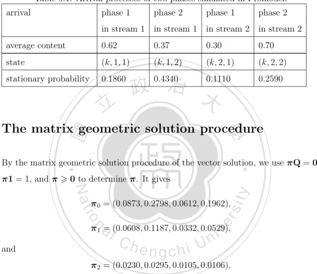
(36) π ¯i. π ¯0. π ¯1. π ¯2. π ¯3. π ¯4. π ¯5. π ¯6. MA. 0.1429. 0.2143. 0.1607. 0.1205. 0.0904. 0.0678. 0.0508. RA. 0.1429. 0.2143. 0.1607. 0.1205. 0.0904. 0.0678. 0.0508. LU. 0.1429. 0.2143. 0.1607. 0.1205. 0.0904. 0.0678. 0.0508. π ¯i. π ¯7. π ¯8. π ¯9. π ¯10. π ¯11. π ¯12. π ¯13. MA. 0.0381. 0.0286. 0.0214. 0.0160. 0.0121. 0.0090. 0.0068. RA. 0.0381. 0.0286. 0.0214. 0.0160. 0.0121. 0.0090. 0.0068. LU. 0.0381. 0.0286. 0.0214. 0.0160. 0.0121. 0.0090. 0.0068. Then we take the example as an M/M/2 queueing model. We find the probability of idle system is 0.142857. The value is the same as π ¯0 .. 政 治 大 15/20 = 0.75. We estimate the values by using 1 − π ¯ − 立. In M/M/2 queues, we find that the busy rate of the queueing is (λ1 +γ1 )/(2µ) = 0. 1 π ¯ . 2 1. The busy rate of the. ‧ 國. 學. queueing is 1 − 0.1429 − 21 × 0.2143 = 0.74995 + 0.75. All results are consistent with the standards of the classic model.. ‧. sit. y. Nat. The stationary probabilities of the states of the. n. al. er. io. arrival process. Ch. i n U. v. Then, we consider the system with two servers, where parameters of arrival processes. engchi. are given by (λ1 , p, λ2 ) = (10, 0.4, 10), (γ1 , p, γ2 ) = (20, 0.4, 5), and let µ = 10. The stationary probabilities of the states of the arrival process, θ, are obtained from its Markovian arrival process representation. By solving the following equations θ(B00 + C) = 0 and θ1 = 1 with Matlab [13], we have θ = (0.1838, 0.4412, 0.1103, 0.2647). For comparison of estimated values θ, we also use a simulation programming of queueing models, Promodel [14]. From the stationary probabilities obtained by simulation with Promodel, the results are shown in Table 5.1.. 28.
(37) We have the values θ = ( 0.1860, 0.4340, 0.1110, 0.2590). We can find that the value is close to π 0 + π 1 + π 2 + π 3 + . . . = π 0 + π 1 + π 2 (I − R)−1 = (0.1838, 0.4412, 0.1103, 0.2647).. Table 5.1: Arrival processes of two phases simulated in Promodel. arrival. phase 1. phase 2. phase 1. phase 2. in stream 1 in stream 1 in stream 2 in stream 2 average content. 0.62. 0.37. 0.30. 0.70. state. (k, 1, 1). (k, 1, 2). (k, 2, 1). (k, 2, 2). stationary probability. 0.1860. 立. 0.4340 0.1110 政 治 大. 0.2590. ‧ 國. 學. The matrix geometric solution procedure. ‧. By the matrix geometric solution procedure of the vector solution, we use πQ = 0,. sit. y. Nat. π1 = 1, and π > 0 to determine π. It gives. io. n. al. er. π 0 = (0.0873, 0.2798, 0.0612, 0.1962),. v. π 1 = (0.0608, 0.1187, 0.0332, 0.0529),. and. Ch. engchi. i n U. π 2 = (0.0230, 0.0295, 0.0105, 0.0106), which are consistent with the numerical results of simulation in Promodel.. Ramaswami’s formula With RA method [7], we have π 0 = (0.0874, 0.2798, 0.0613, 0.1962), π 1 = (0.0608, 0.1186, 0.0333, 0.0528),. 29.
(38) and π 2 = (0.0229, 0.0293, 0.0105, 0.0104), which will be compared with simulation, LU approach in the next section.. LU factorization Next, by applying the algorithm of LU factorization, it gives π 0 = (0.0873, 0.2798, 0.0612, 0.1962),. 政 治 大. π 1 = (0.0608, 0.1187, 0.0332, 0.0529),. 立. and. π 2 = (0.0230, 0.0295, 0.0105, 0.0106),. ‧ 國. 學 ‧. Numerical experiments by changing p. y. Nat. sit. Here, we observe the numerical results of changing values of p, and other variables. n. al. i n U. and 0 6 p < 0.8840, where p = 0.1, 0.2, 0.3, 0.4, 0.5, 0.6.. Ch. engchi. er. io. are fixed. That is, it gives (λ1 , p, λ2 ) = (10, p, 10), (γ1 , p, γ2 ) = (20, p, 5), µ = 10,. v. The numerical results are compared in three different approaches, MA represents the matrix geometric solution procedure, RA represents Ramaswami’s formula, and LU represents LU factorization. Let π ¯i be the probability of i customers in system, i.e., π ¯i = π i 1. Table 5.2 and Table 5.3 shows the comparison of numerical results.. Promodel In order to estimate the π 0 , π 1 and π 2 accurately. By simulation in Promodel [14], it gives the queue empty rates which are shown in Table 5.4. Here, the. 30.
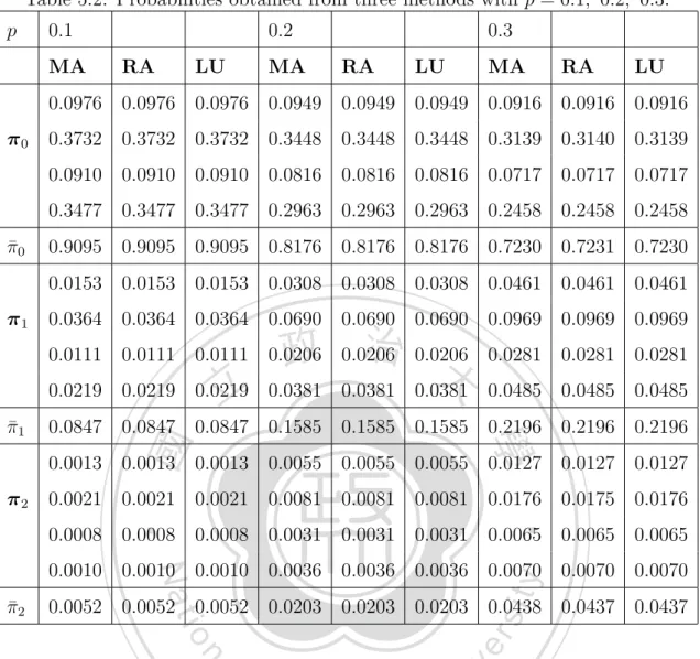
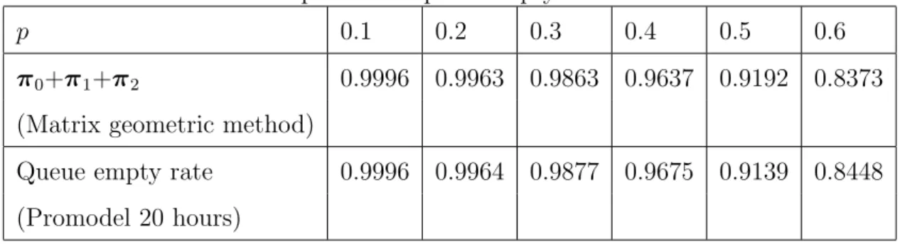
(39) Table 5.2: Probabilities obtained from three methods with p = 0.1, 0.2, 0.3. p. 0.1 MA. 0.2 RA. LU. 0.3. MA. RA. LU. MA. RA. LU. 0.0976 0.0976 0.0976 0.0949 0.0949 0.0949 0.0916 0.0916 0.0916 π0. 0.3732 0.3732 0.3732 0.3448 0.3448 0.3448 0.3139 0.3140 0.3139 0.0910 0.0910 0.0910 0.0816 0.0816 0.0816 0.0717 0.0717 0.0717 0.3477 0.3477 0.3477 0.2963 0.2963 0.2963 0.2458 0.2458 0.2458. π ¯0. 0.9095 0.9095 0.9095 0.8176 0.8176 0.8176 0.7230 0.7231 0.7230 0.0153 0.0153 0.0153 0.0308 0.0308 0.0308 0.0461 0.0461 0.0461. π1. 0.0364 0.0364 0.0364 0.0690 0.0690 0.0690 0.0969 0.0969 0.0969. 政 治 大 0.0381 0.0381 0.0381. 0.0111 0.0111 0.0111 0.0206 0.0206 0.0206 0.0281 0.0281 0.0281. 立. 0.0219 0.0219 0.0219. 0.0847 0.0847 0.0847 0.1585 0.1585 0.1585 0.2196 0.2196 0.2196. ‧ 國. 學. π ¯1. 0.0485 0.0485 0.0485. 0.0013 0.0013 0.0013 0.0055 0.0055 0.0055 0.0127 0.0127 0.0127 0.0021 0.0021 0.0021 0.0081 0.0081 0.0081 0.0176 0.0175 0.0176. ‧. π2. 0.0008 0.0008 0.0008 0.0031 0.0031 0.0031 0.0065 0.0065 0.0065. y. sit. 0.0052 0.0052 0.0052 0.0203 0.0203 0.0203 0.0438 0.0437 0.0437. io. n. al. er. π ¯2. Nat. 0.0010 0.0010 0.0010 0.0036 0.0036 0.0036 0.0070 0.0070 0.0070. i n U. v. queue empty rate is referred to the probability of no customer in the queue. We P ¯k is equal to the queue empty rate obtained with simfind that the sum 2k=0 π. Ch. engchi. ulations, where (λ1 , p, λ2 ) = (10, p, 10), (γ1 , p, γ2 ) = (20, p, 5), 0 6 p < 0.8840, p = 0.1, 0.2, 0.3, 0.4, 0.5, 0.6 and µ = 10. The comparison results are shown in Table 5.4 . According to Table 5.2 and Table 5.3, we find that if the value of p is smaller, the π i value of three methods are very close. But when the value of p is closed to its upper bound, the π i ’s are a little different.. 31.
(40) Table 5.3: Probabilities obtained from three methods with p = 0.4, 0.5, 0.6. p. 0.4. 0.5. MA. RA. LU. 0.6. MA. RA. LU. MA. RA. LU. 0.0873 0.0874 0.0873 0.0815 0.0817 0.0815 0.0730 0.0727 0.0730 π0. 0.2798 0.2798 0.2798 0.2410 0.2410 0.2410 0.1956 0.1948 0.1956 0.0612 0.0613 0.0612 0.0500 0.0502 0.0500 0.0379 0.0377 0.0379 0.1962 0.1962 0.1962 0.1478 0.1480 0.1478 0.1014 0.1010 0.1014. π ¯0. 0.6245 0.6247 0.6245 0.5203 0.5209 0.5203 0.4079 0.4062 0.4079. 治 政 大 0.1321 0.1317 0.1321. 0.0608 0.0608 0.0608 0.0739 0.0740 0.0739 0.0832 0.0834 0.0832 π1. 0.1187 0.1186 0.1187. 立. 0.1336 0.1323 0.1336. 0.0332 0.0333 0.0332 0.0354 0.0355 0.0354 0.0338 0.0340 0.0338. ‧ 國. 學. 0.0529 0.0528 0.0529 0.0512 0.0510 0.0512 0.0436 0.0431 0.0436 π ¯1. 0.2656 0.2655 0.2656 0.2926 0.2922 0.2926 0.2942 0.2938 0.2942. 0.0295 0.0293 0.0295 0.0423 0.0417 0.0423 0.0533 0.0515 0.0533. y. Nat. π2. ‧. 0.0230 0.0229 0.0230 0.0360 0.0360 0.0360 0.0505 0.0504 0.0505. sit. 0.0105 0.0105 0.0105 0.0145 0.0145 0.0145 0.0173 0.0162 0.0173. al. n. π ¯2. er. io. 0.0106 0.0104 0.0106 0.0133 0.0129 0.0133 0.0142 0.0135 0.0142. i n U. v. 0.0736 0.0731 0.0736 0.1061 0.1051 0.1061 0.1353 0.1326 0.1353. Ch. engchi. Table 5.4: Comparison of queue empty rates of two servers. p. 0.1. 0.2. 0.3. 0.4. 0.5. 0.6. π 0 +π 1 +π 2. 0.9996 0.9963 0.9863 0.9637 0.9192 0.8373. (Matrix geometric method) Queue empty rate. 0.9996 0.9964 0.9877 0.9675 0.9139 0.8448. (Promodel 20 hours). 32.
(41) Inter-departure times The departure process has three different partitions: First, when there is no customer in the system, a departure has to wait until at least one customer has occurred followed by a service. Second, when there is one customer in the system, the inter-departure time can be a function of single processing customer ’s remaining service or it could evolve from a customer arrived and its completion of service. Third, when a departing customer leaves the system with at least two remaining. 政 治 大. customers, the minimum of the remaining service time of one of these customers or. 立. complete service time of another customer becomes the inter-departure time.. ‧ 國. 學. Now, we begin by describing the two arrival processes (λ1 , p, λ2 ) = (10, 0.4, 10), (γ1 , p, γ2 ) = (20, 0.4, 5), and let µ = 10.. ‧. Then, we find that when there remain at least two customers in the system,. Nat. sit. y. the inter-departure time characteristics are the same for all these cases (k ≥ 2).. io. al. n. segmentations given by. er. The infinitesimal generator matrix for the departure process G21 has three different. Ch. G21 =. i n U2 +. e n0g c 1h i. 0. B00. C. 0. 1. 0. B11. b C. 2+. 0. 0. SSin. where. . 12. . 4 b , C=C·1= 8 0 h i SSin = S1 ⊕ S1 = −20 .. 33. ,. v.
(42) Thus, we have . G21. −30. 5 10 0 = 0 0 0 0 0. 12. 6. 0. 12. 0. 0. 0. 0. . −15 0 6 0 4 0 0 0 0 −30 12 0 0 8 0 0 10 5 −15 0 0 0 0 0 0 0 0 −40 12 6 0 12 . 0 0 0 5 −25 0 6 4 0 0 0 10 0 −40 12 8 0 0 0 0 10 5 −25 0 0 0 0 0 0 0 0 −20. 政 治 大 The probabilities of the departure-process system starting in the various states 立. ‧ 國. 學. d = (d0 , d1 , d2+ ) are made up of the departure point probabilites, with d0 = π 1 A10 /λ,. ‧. d1 = π 2 A21 /λ,. y. n=3. al. n. This series can be written in closed form as. Ch. ∞ X. d2+ = (. er. io. sit. Nat. d2+. ∞ X =( π n A/λ)1.. i n U. v. i e nπgRc hA/λ)1, 2. n−2. n=3. = π 2 [(I − R)−1 − I]A/λ)1. By above equations. We can compute d : d0 = (0.1253, 0.2446, 0.0685, 0.1090), d1 = (0.0946, 0.1215, 0.0434, 0.0436), d2+ = 0.1495.. 34.
(43) Moments of inter-departure times The stationary inter-departure time is of the phase type distribution characterized by [d, G21 ]. Thus, from Neuts [8] we know that the moments of inter-departure times random variable X are given by E[X] = (−1)d(G21 )−1 1. Then we use different p to compute E[X] by Matlab and Promodel : p. 0.1. 0.2. 0.3. 0.4. 0.5. E[X] Matlab. 1.0405 0.4846 0.2991 0.2061 0.1500 0.1123. E[X] Promodel. 1.00. 治 政 0.49 0.30 0.21 大. 立. 0.15. 0.6. 0.11. 學. V ar[X] = E[X 2 ] − E[X]2 . 0.1. 0.2. 0.3. ‧. p. ‧ 國. and we use the same parameters to compute V ar[X] by Matlab and Promodel,. 0.4. 0.5. 0.6. V ar[X] Promodel. 1.1484 0.2796 0.1339 0.0559 0.0344 0.0156. er. io. sit. y. 1.1703 0.2711 0.1091 0.0541 0.0295 0.0167. Nat. V ar[X] Matlab. a. n. v. i departures Lagk correlations lbetween successive n Ch engchi U To get the lagk correlations of the output inter-departure times, it is necessary to c2 segmented into two matrices: the indevelop the infinitesimal generator matrix G ternal transitions (without departures) G21 and the matrix containing the departure c2 = G21 + G22 . transition G22 such that G The matrix G22 is characterized as. G22 =. 0. 1. 2+. 0. 0. 0. 0. 1. A10. 0. 0. 2+. 0. b 21 (1 − t)A. tSSout. 35. ,.
(44) where t is the probability that departure leaves the system with at least two customers remaining and (1 − t) is the probability that only one customer remains. We define t as P∞ π 1 d2+ d2+ a=3 P∞ a = = = 0.3303. t= π 2 1 + a=3 π a 1 d1 + d2+ 1 − d0 1 Two of sub-matrices in G22 are given by b 21 = θ ⊗ (S1o ⊕ S1o ) = [0.1838, 0.4412, 0.1103, 0.2647] ⊗ [20], A SSout = S1o ⊕ S1o = [20].. 0. 0. 0. 0. 0. 0. 0. 0. 0. 0. 0. 0. 0. 0. 0. 0. 0. 0. 10. 0. 0. 0. 0. 10. 0. 0. 0. 10. 0. 0. n. 0. 0. 0. 0. 0. 0. 0. 0. 0. 0. 0. 0. 0. 0. 0. 0. 0. 0. 0. 0. 0. 0. 0. y. 0. io. 0. ‧. 0. 0. 學. 0. 0. 0. 0. 0. 0. sit. 0. er. 0. 政 治 大. Nat. G22. = . 立 0 0. ‧ 國. Thus, we have . a l 10 0 0 0 v 0 i n 0 0C 2.4620 U 3.5453 h e n g5.9088 c h i 1.4772 0. 0 6.6066. . . Given G21 and G22 matrices, from Bodrog, Horvath, Telek [2], and Telek, Horvath [11], we have that the lagk correlation is computed by lagk =. (λ)2 d(−G21 )−1 ((−G21 )−1 G22 )k (−G21 )−1 1 − 1 , 2(λ)2 d(−G21 )−2 1 − 1). where λ = (p[( λ11 p + ( λ11 +. 1 )(1 λ2. − p)]−1 + p[( γ11 p + ( γ11 +. 1 )(1 γ2. − p)]−1 = 4.8529) is. the average effective arrival rate. We can compute lagk (k = 1, 2, 3, 4), lag1 = 0.0342, lag2 = 0.0224, lag3 = 0.0206, lag4 = 0.0203.. 36.
(45) 5.2. Queueing models with three servers. M/M/3 queueing models Once more, we present a numerical example of M/M/3 queues to verify our model. Here, two arrival processes (λ1 , p, λ2 ) and (γ1 , p, γ2 ) are given with (λ1 , p, λ2 ) = (10, 1, 10), (γ1 , p, γ2 ) = (5, 1, 20), and µ = 10. By applying the MA, RA, and LU methods, we take π ¯0 π ¯1 · · · π ¯12 π ¯13 to compare the values. We find that they are the same. π ¯3. π ¯4. π ¯5. π ¯6. 0.2105. 0.3158. 0.1184. 0.0592. 0.0296. 0.0148. RA. 0.2105. 0.3158. 0.2368. 0.1184. 0.0592. 0.0296. 0.0148. LU. 0.2105. 0.3158. 0.2368. 0.1184. 0.0592. 0.0296. π ¯i. π ¯7. π ¯8. π ¯9. π ¯10. π ¯11. π ¯12. π ¯13. MA. 0.0074. 0.0037. 0.0018. 0.0009. 0.0005. 0.0002. 0.0001. RA. 0.0074. 0.0037. 0.0018. 0.0009. 0.0005. 0.0002. 0.0001. LU. 0.0074. 0.0037. 0.0018. 0.0009. 0.0005. 0.0002. 0.0001. 立. 0.2368. 0.0148. Nat. y. MA. 政 治 大. sit. π ¯2. ‧ 國. π ¯1. ‧. π ¯0. 學. π ¯i. n. al. er. io. In this example, we find the probability of idle system is 0.210526, which is. iv n U π ¯ − π ¯ , it gives the busy rate. the same as π ¯0 . In M/M/3 queues, we know that the busy rate of the queueing is. Ch. engchi. (λ1 + γ1 )/(3µ) = 15/30 = 0.5. By using 1 − π ¯0 − of queues as follows 1 − 0.2105 −. 2 3 1. 1 3 2. 1 2 × 0.3158 − × 0.2368 + 0.5263 + 0.5. 3 3. The matrix geometric solution procedure Here, we present numerical results of queueing systems with three servers, where two arrival processes are given with (λ1 , p, λ2 ) = (10, 0.4, 10), (γ1 , p, γ2 ) = (20, 0.4, 5), and let µ = 10.. 37.
(46) From the matrix geometric solution procedure, we solve πQ = 0, π1 = 1, and π > 0 to estimate π. Then, it gives the vector solution π 0 = (0.0887, 0.2838, 0.0622, 0.1988), π 1 = (0.0621, 0.1204, 0.0339, 0.0534), π 2 = (0.0240, 0.0297, 0.0109, 0.0103), and π 3 = (0.0066, 0.0056, 0.0026, 0.0017).. 治. Ramaswami’s formula 政. 立. 大. π 0 = (0.0887, 0.2838, 0.0622, 0.1988),. Nat. n. al. er. io. and. sit. π 2 = (0.0240, 0.0297, 0.0109, 0.0103),. y. π 1 = (0.0621, 0.1204, 0.0339, 0.0534),. ‧. ‧ 國. 學. By applying RA method, we have. v. π 3 = (0.0066, 0.0056, 0.0026, 0.0017).. Ch. engchi. i n U. LU factorization By using LU factorization given in previous section, we obtain π 0 = (0.0887, 0.2838, 0.0622, 0.1988), π 1 = (0.0621, 0.1204, 0.0339, 0.0534), π 2 = (0.0240, 0.0297, 0.0109, 0.0103), and π 3 = (0.0066, 0.0056, 0.0026, 0.0017).. 38.
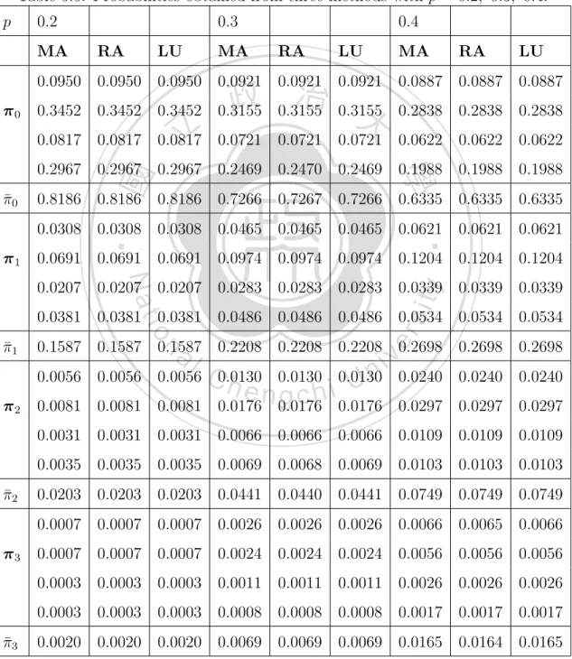
(47) Numerical experiments by changing p We observe the effect of changing p on the numerical results obtained from three methods. Here, we have (λ1 , p, λ2 ) = (10, p, 10), (γ1 , p, γ2 ) = (20, p, 5), µ = 10, and 0 6 p < w = 1, for p = 0.2, 0.3, 0.4, 0.5, 0.6, 0.7, 0.8, 0.9. Tables 5.5-5.7 show the comparison of numerical results. Table 5.5: Probabilities obtained from three methods with p = 0.2, 0.3, 0.4. p. 0.2 MA. 0.3 RA. LU. MA. 0.4 RA. LU. MA. RA. LU. 政 治 大. 0.0950 0.0950 0.0950 0.0921 0.0921 0.0921 0.0887 0.0887 0.0887 π0. 0.3452 0.3452 0.3452 0.3155 0.3155 0.3155 0.2838 0.2838 0.2838. 立. 0.0817 0.0817 0.0817 0.0721 0.0721 0.0721 0.0622 0.0622 0.0622. ‧ 國. π ¯0. 學. 0.2967 0.2967 0.2967 0.2469 0.2470 0.2469 0.1988 0.1988 0.1988 0.8186 0.8186 0.8186 0.7266 0.7267 0.7266 0.6335 0.6335 0.6335. π1. ‧. 0.0308 0.0308 0.0308 0.0465 0.0465 0.0465 0.0621 0.0621 0.0621 0.0691 0.0691 0.0691 0.0974 0.0974 0.0974 0.1204 0.1204 0.1204. y. Nat. sit. 0.0207 0.0207 0.0207 0.0283 0.0283 0.0283 0.0339 0.0339 0.0339. er. al. 0.1587 0.1587 0.1587 0.2208 0.2208 0.2208 0.2698 0.2698 0.2698. n. π ¯1. io. 0.0381 0.0381 0.0381 0.0486 0.0486 0.0486 0.0534 0.0534 0.0534. Ch. 0.0056 0.0056 0.0056 0.0130 0.0130 π2. 0.0081 0.0081 0.0081. i n 0.0130 U. e n g c h i 0.0176 0.0176 0.0176. v. 0.0240 0.0240 0.0240 0.0297 0.0297 0.0297. 0.0031 0.0031 0.0031 0.0066 0.0066 0.0066 0.0109 0.0109 0.0109 0.0035 0.0035 0.0035 0.0069 0.0068 0.0069 0.0103 0.0103 0.0103 π ¯2. 0.0203 0.0203 0.0203 0.0441 0.0440 0.0441 0.0749 0.0749 0.0749 0.0007 0.0007 0.0007 0.0026 0.0026 0.0026 0.0066 0.0065 0.0066. π3. 0.0007 0.0007 0.0007 0.0024 0.0024 0.0024 0.0056 0.0056 0.0056 0.0003 0.0003 0.0003 0.0011 0.0011 0.0011 0.0026 0.0026 0.0026 0.0003 0.0003 0.0003 0.0008 0.0008 0.0008 0.0017 0.0017 0.0017. π ¯3. 0.0020 0.0020 0.0020 0.0069 0.0069 0.0069 0.0165 0.0164 0.0165. 39.
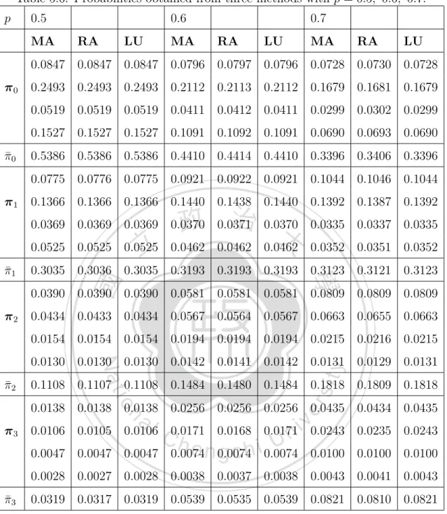
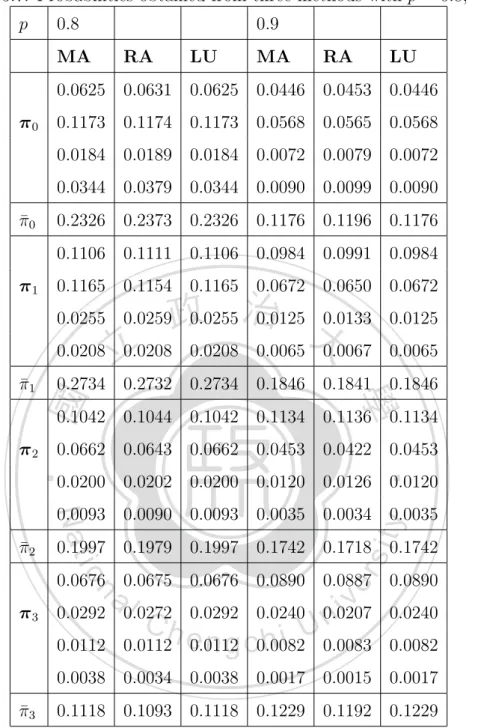
(48) Table 5.6: Probabilities obtained from three methods with p = 0.5, 0.6, 0.7. p. 0.5 MA. 0.6 RA. LU. 0.7. MA. RA. LU. MA. RA. LU. 0.0847 0.0847 0.0847 0.0796 0.0797 0.0796 0.0728 0.0730 0.0728 π0. 0.2493 0.2493 0.2493 0.2112 0.2113 0.2112 0.1679 0.1681 0.1679 0.0519 0.0519 0.0519 0.0411 0.0412 0.0411 0.0299 0.0302 0.0299 0.1527 0.1527 0.1527 0.1091 0.1092 0.1091 0.0690 0.0693 0.0690. π ¯0. 0.5386 0.5386 0.5386 0.4410 0.4414 0.4410 0.3396 0.3406 0.3396 0.0775 0.0776 0.0775 0.0921 0.0922 0.0921 0.1044 0.1046 0.1044. π1. 0.1366 0.1366 0.1366 0.1440 0.1438 0.1440 0.1392 0.1387 0.1392. 政 治 大 0.0462 0.0462 0.0462. 0.0369 0.0369 0.0369 0.0370 0.0371 0.0370 0.0335 0.0337 0.0335. 立. 0.0525 0.0525 0.0525. 0.3035 0.3036 0.3035 0.3193 0.3193 0.3193 0.3123 0.3121 0.3123. ‧ 國. 學. π ¯1. 0.0352 0.0351 0.0352. 0.0390 0.0390 0.0390 0.0581 0.0581 0.0581 0.0809 0.0809 0.0809 0.0434 0.0433 0.0434 0.0567 0.0564 0.0567 0.0663 0.0655 0.0663. ‧. π2. 0.0154 0.0154 0.0154 0.0194 0.0194 0.0194 0.0215 0.0216 0.0215. y. sit. 0.1108 0.1107 0.1108 0.1484 0.1480 0.1484 0.1818 0.1809 0.1818. io. er. π ¯2. Nat. 0.0130 0.0130 0.0130 0.0142 0.0141 0.0142 0.0131 0.0129 0.0131. 0.0138 0.0138 0.0138 0.0256 0.0256 0.0256 0.0435 0.0434 0.0435. al. n. π3. Ch. i n U. v. 0.0106 0.0105 0.0106 0.0171 0.0168 0.0171 0.0243 0.0235 0.0243. engchi. 0.0047 0.0047 0.0047 0.0074 0.0074 0.0074 0.0100 0.0100 0.0100 0.0028 0.0027 0.0028 0.0038 0.0037 0.0038 0.0043 0.0041 0.0043 π ¯3. 0.0319 0.0317 0.0319 0.0539 0.0535 0.0539 0.0821 0.0810 0.0821. 40.
(49) Table 5.7: Probabilities obtained from three methods with p = 0.8, 0.9. p. 0.8. 0.9. MA. RA. LU. MA. RA. LU. 0.0625 0.0631 0.0625 0.0446 0.0453 0.0446 π0. 0.1173 0.1174 0.1173 0.0568 0.0565 0.0568 0.0184 0.0189 0.0184 0.0072 0.0079 0.0072 0.0344 0.0379 0.0344 0.0090 0.0099 0.0090. π ¯0. 0.2326 0.2373 0.2326 0.1176 0.1196 0.1176 0.1106 0.1111 0.1106 0.0984 0.0991 0.0984. π1. 0.1165 0.1154 0.1165 0.0672 0.0650 0.0672. 政 治 大 0.0208 立 0.0208 0.0208 0.0065 0.0067. 0.0255 0.0259 0.0255 0.0125 0.0133 0.0125. 0.2734 0.2732 0.2734 0.1846 0.1841 0.1846. ‧ 國. 學. π ¯1. 0.0065. 0.1042 0.1044 0.1042 0.1134 0.1136 0.1134 0.0662 0.0643 0.0662 0.0453 0.0422 0.0453. ‧. π2. 0.0200 0.0202 0.0200 0.0120 0.0126 0.0120. y. sit. 0.1997 0.1979 0.1997 0.1742 0.1718 0.1742. io. er. π ¯2. Nat. 0.0093 0.0090 0.0093 0.0035 0.0034 0.0035. 0.0676 0.0675 0.0676 0.0890 0.0887 0.0890. al. n. π3. Ch. i n U. v. 0.0292 0.0272 0.0292 0.0240 0.0207 0.0240. engchi. 0.0112 0.0112 0.0112 0.0082 0.0083 0.0082 0.0038 0.0034 0.0038 0.0017 0.0015 0.0017 π ¯3. 0.1118 0.1093 0.1118 0.1229 0.1192 0.1229. Promodel We compare the values of. P3. k=0. π ¯k with the queue empty rate obtained by using. simulation in ProModel. The variable values are given as (λ1 , p, λ2 ) = (10, p, 10), (γ1 , p, γ2 ) = (20, p, 5), and p varies from 0.2 to 0.9, with µ = 10. Table 5.8 shows. 41.
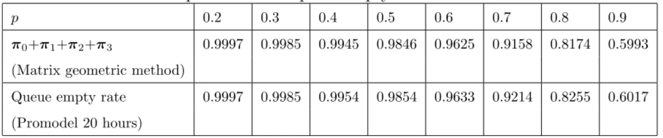
(50) the comparison of numerical results. Table 5.8: Comparison of the queue empty rates of three servers. p. 0.2. 0.3. 0.4. 0.5. 0.6. 0.7. 0.8. 0.9. π 0 +π 1 +π 2 +π 3. 0.9997. 0.9985. 0.9945. 0.9846. 0.9625. 0.9158. 0.8174. 0.5993. 0.9997. 0.9985. 0.9954. 0.9854. 0.9633. 0.9214. 0.8255. 0.6017. (Matrix geometric method) Queue empty rate (Promodel 20 hours). It shows the same situation like the queueing with two servers. According to Tables 5.5-5.7, we find that if the value of p is smaller, the π i value of three methods. 政 治 大. are very close. But when the value of p is closed to its upper bound, the π i ’s are a little different.. 學. ‧ 國. 立. Inter-departure times. ‧. Now, we begin by describing the two arrival processes as (λ1 , p, λ2 ) = (10, 0.4, 10),. Nat. sit. y. (γ1 , p, γ2 ) = (20, 0.4, 5), and µ = 10.. er. io. Then, we find that when there remain at least three customers in the system,. al. n. v i n C hfor the departureUprocess G The infinitesimal generator matrix engchi. the inter-departure time characteristics are the same for all these cases (k ≥ 3).. segmentations are given by. G31 =. 0. 1. 2. 3+. 0. B00. C. 0. 0. 1. 0. B11. C. 0. 2. 0. 0. B22. b C. 3+. 0. 0. 0. SSin. 42. ,. 31. has three different.
(51) where sub-matrices given by . . 12. 4 b , C=C·1= 8 0 SSin = S1 ⊕ S1 ⊕ S1 =. h. −30. i. .. Thus, we have −30 12 6 0 12 0 0 0 0 0 0 0 0 5 −15 0 6 0 4 0 0 0 0 0 0 0 10 0 −30 12 0 0 8 0 0 0 0 0 0 0 10 5 −15 0 0 0 0 0 0 0 0 0 0 0 0 0 −40 12 6 0 12 0 0 0 0 0 0 0 0 5 −25 0 6 0 4 0 0 0 G31 = 0 0 0 0 10 0 −40 12 0 0 8 0 0 0 0 0 0 0 10 5 −25 0 0 0 0 0 0 0 0 0 0 0 0 0 −50 12 6 0 12 0 0 0 0 0 0 0 0 5 −35 0 6 4 0 0 0 0 0 0 0 0 10 0 −50 12 8 0 0 0 0 0 0 0 0 0 10 5 −35 0 0 0 0 0 0 0 0 0 0 0 0 0 −30. 立. 政 治 大. ‧. ‧ 國. 學. n. er. io. sit. y. Nat. al. Ch. engchi. i n U. v. The probabilities of the departure-process system starting in the various states d = (d0 , d1 , d2 , d3+ ) are made up of the departure point probabilites, with. d0 = π 1 A10 /λ, d1 = π 2 A21 /λ, d2 = π 3 A32 /λ, d3+. ∞ X =( π n A/λ)1. n=4. 43. . .
(52) This series can be written in closed form as d3+. ∞ X =( π 3 Rn−3 A/λ)1 n=4. = π 3 [(I − R)−1 − I]A/λ)1. By above equations. We can compute d d0 = (0.1280, 0.2480, 0.0698, 0.1100) d1 = (0.0989, 0.1226, 0.0448, 0.0424) d2 = (0.0407, 0.0347, 0.0158, 0.0105). 治 政 d = 0.0338 大 3+. Moments of inter-departure times. 學. ‧ 國. 立. ‧. The stationary inter-departure time is of the phase type distribution characterized. Nat. sit. y. by [d, G31 ]. Thus, from Neuts [8] we know that the moments of inter-departure. io. er. times random variable X are given by. n. a l E[X] = (−1)d(G ) 1. i v n Ch U engchi 31. −1. Then we use different p to compute E[X] by Matlab and Promodel : p. 0.2. 0.3. 0.4. 0.5. 0.6. 0.7. 0.8. 0.9. E[X] Matlab. 0.4846. 0.2991. 0.2061. 0.1500. 0.1123. 0.0851. 0.0643. 0.0475. E[X] Promodel. 0.50. 0.31. 0.21. 0.15. 0.11. 0.08. 0.06. 0.04. and we use the same parameters to compute V ar[X] by Matlab and Promodel, V ar[X] = E[X 2 ] − E[X]2 . p. 0.2. 0.3. 0.4. 0.5. 0.6. 0.7. 0.8. 0.9. V ar[X] Matlab. 0.2712. 0.1093. 0.0543. 0.0299. 0.0172. 0.0099. 0.0055. 0.0027. V ar[X] Promodel. 0.32. 0.1176. 0.0516. 0.0344. 0.0156. 0.0119. 0.0051. 0.0025. 44.
(53) Lagk correlations between successive departures To get the lagk correlations of the output inter-departure times, it is necessary to c3 segmented into two matrices: the indevelop the infinitesimal generator matrix G ternal transitions (without departures) G31 and the matrix containing the departure c3 = G31 + G32 . transition G32 such that G The matrix G32 is characterized as. G32 =. 0. 1. 2. 3+. 0. 0. 0. 0. 0. 1. A10. 2 立 3 +. 政0 治 0 大 0 A 0. 0. 21. 0. b 32 (1 − t) A. 0. ,. 0. tSSout. ‧ 國. 學. where t is the probability that departure leaves the system with at least three cus-. ‧. tomers remaining. We compute t as P∞ π 1 d3+ d3+ a=4 P∞ a = = 0.2494. = t= π 3 1 + a=4 π a 1 d2 1 + d3+ 1 − d0 1 − d1 1. n. Ch. er. io. al. sit. y. Nat. Two of these sub-matrices are given by. i n U. v. b 32 = θ ⊗ (S1o ⊕ S1o ⊕ S1o ) = [0.1838, 0.4412, 0.1103, 0.2647] ⊗ [30], A. engchi. SSout = S1o ⊕ S1o ⊕ S1o = [30]. Thus, we have. 45.
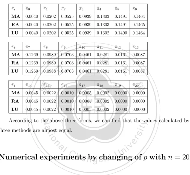
(54) . 0. 0. 0. 0. 0. 0. 0. 0. 0. 0. 0. 0. 0. 0. 0. 0. 0. 0. 0. 0. 0. 0. 0. 0. 0. 0. 0. 0. 0. 0. 0. 0. 0. 0. 0. 0. 0. 0. 0. 0. 0. 0. 0. 0. 0. 0. 0. 0. 0. 0. 0. 0. 10. 0. 0. 0. 0. 0. 0. 0. 0. 0. 0. 0. 0. 0. 10. 0. 0. 0. 0. 0. 0. 0. 0. 0. 0. 0. 0. 0. 10. 0. 0. 0. 0. 0. 0. 0. 0. 0. 0. 0. 0. 0. 10. 0. 0. 0. 0. 0. 0. 0. 0. 0. 0. 0. 0. 0. 20. 0. 0. 0. 0. 0. 0. 0. 0. 0. 0. 0. 0. 0. 20. 0. 0. 0. 0. 0. 0. 0. 0. 0. 0. 0. 0. 0. 0. 0. 0. 0. 0. 0. 0. 0. 0. 0. 0. 0. 0. 立0 0. 0 20 治 0 0 政 大 0 0 0 20 0 0. 0. 0. 0. 4.1391 9.9339 2.4835 5.9604 7.4831. 學. ‧ 國. G32. = . Given G31 and G32 matrices, from Bodrog, Horvath, Telek [2], and Telek, Hor-. 1 )(1 λ2. al. − p)]−1 + p[( γ11 p + ( γ11 +. 1 )(1 γ2. − p)]−1 = 4.8529) is. er. io. where λ = (p[( λ11 p + ( λ11 +. sit. y. (λ)2 d(−G31 )−1 ((−G31 )−1 G32 )k (−G31 )−1 1 − 1 , 2(λ)2 d(−G31 )−2 1 − 1). Nat. lagk =. ‧. vath [11], we have that the lagk correlation is computed by. v. n. the average effective arrival rate. We can compute lagk (k = 1, 2, 3, 4),. Ch. engchi. i n U. lag1 = 0.0344, lag2 = 0.0133, lag3 = 0.0111, lag4 = 0.0106.. 5.3. Queueing models with more than twenty servers. With twenty servers Here, we present numerical results of queueing systems with twenty servers. The parameters of two arrival processes are given with (λ1 , p, λ2 ) = (10, 0.4, 10), (γ1 , p, γ2 ) = (20, 0.4, 5), and let µ = 0.8.. 46. . .
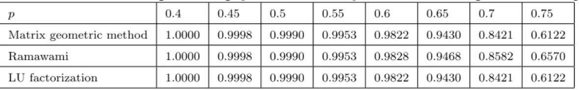
(55) The numerical results are compared in three different approaches, MA represents matrix geometric solution procedure, RA represents Ramaswami’s formula, and LU represents LU factorization. Then, it gives the solutions. π ¯i. π ¯0. π ¯1. π ¯2. π ¯3. π ¯4. π ¯5. π ¯6. MA. 0.0040. 0.0202. 0.0525. 0.0939. 0.1303. 0.1491. 0.1464. RA. 0.0040. 0.0202. 0.0525. 0.0939. 0.1303. 0.1491. 0.1465. LU. 0.0040. 0.0202. 0.0525. 0.0939. 0.1302. 0.1490. 0.1464. π ¯i. π ¯7. π ¯8. π ¯9. π ¯10. π ¯11. π ¯12. π ¯13. MA. 0.1269. 0.0989. 0.0703. RA. 0.1269. 0.0989. 0.0703. LU. 0.1269. 0.0988. π ¯i. π ¯14. π ¯15. MA. 0.0045. RA LU. 政 治 大 0.0281. 0.0161. 0.0087. 0.0461. 0.0281. 0.0161. 0.0087. 0.0461. 0.0281. 0.0161. 0.0087. π ¯16. π ¯17. π ¯18. π ¯19. π ¯20. 0.0022. 0.0010. 0.0005. 0.0002. 0.0000. 0.0045. 0.0022. 0.0010. 0.0005. 0.0002. 0.0000. 0.0000. 0.0045. 0.0022. 0.0010. 0.0005. 0.0002. 0.0000. 0.0000. 0.0703. 0.0000. ‧. ‧ 國. 立. 學. 0.0461. sit. y. Nat. According to the above three forms, we can find that the values calculated by. io. n. al. er. three methods are almost equal.. i n U. C. v. h e nbyg cchanging Numerical experiments of p with n = 20 hi Next, we consider the system with twenty servers, where p varies from 0 to 0.75. Here, parameters of arrival processes are given by (λ1 , p, λ2 ) = (10, p, 10), (γ1 , p, γ2 ) = (20, p, 5), and let µ = 0.8. By Lemma 1, we have 0 6 p < w = 0.8098. Table 5.9 shows the comparison of numerical results with three different methods.. 47.
數據
+7
相關文件
We would like to point out that unlike the pure potential case considered in [RW19], here, in order to guarantee the bulk decay of ˜u, we also need the boundary decay of ∇u due to
Primal-dual approach for the mixed domination problem in trees Although we have presented Algorithm 3 for finding a minimum mixed dominating set in a tree, it is still desire to
The function f (m, n) is introduced as the minimum number of lolis required in a loli field problem. We also obtained a detailed specific result of some numbers and the upper bound of
Let f being a Morse function on a smooth compact manifold M (In his paper, the result can be generalized to non-compact cases in certain ways, but we assume the compactness
The main tool in our reconstruction method is the complex geometri- cal optics (CGO) solutions with polynomial-type phase functions for the Helmholtz equation.. This type of
Then, a visualization is proposed to explain how the convergent behaviors are influenced by two descent directions in merit function approach.. Based on the geometric properties
In this chapter we develop the Lanczos method, a technique that is applicable to large sparse, symmetric eigenproblems.. The method involves tridiagonalizing the given
Matrix model recursive formulation of 1/N expansion: all information encoded in spectral curve ⇒ generates topological string amplitudes... This is what we
