摘要
近年來許多文獻研究顯示,於小應變量下,土壤之力學行為對土壤及結構互 制問題之分析有極重要的影響。本研究基於此目的,致力於發展一套具有進行極 小應變力學試驗能力之試驗系統。於此系統中,採用最新加載設備。以精密軸向 應力、應變控制達到小應變試驗之目的。軸向傳導裝置應用高精密、零背隙滾珠 螺桿,避免於軸向位移傳遞過程中發生誤差。並研發數位壓力控制器,提供準確 之壓力來源。另外於設計概念上,克服並改善操作便利性,大量使用圖像式人機 介面,使試驗系統單純化。最後,運用新一代 LabVIEW 程式撰寫試驗系統,提 供一多功能平台,使所有使用者依其特殊目的而增加或修改試驗系統。且於報告 中提出相關模式之建立,以及考量土壤小應變下應力應變行為之工程案例分析。
Abstract
According to many research results in last few decades, the soil properties at small strain is an important factor of analyzing the geotechnical engineering problems.
For that purpose, the testing system could perform small-strain tests must be set up. In order to bring out the soil properties realistically, the testing system should be as precise as possible. Therefore, there was a whole new triaxial testing system introduced in this research.
The new testing system designed in this study was separated into three major parts, i.e. loading system, pressure control system, and data acquisition system. The loading system was consisted of a high-performance servo motor and extreme precise ball screw. And the attainable minimum axial displacement was dependent on the performance of the loading system. Besides the accurate control of axial load and displacement, the pressure source is quite important too. The pressure source in this testing system is two digital pressure controller design and manufacture in Taiwan.
The digital pressure controller could provide steady and continuous pressure for all tests. At last, the sensors used in measuring all changes of the specimen are very sensitive and the DAQ devices have exceedingly high resolution.
Furthermore, the testing program was programmed in LabVIEW—the new and versatile program. It provides a convenient way for users to modify the testing program to meet their needs. The small strain anisotropic triaxial testing system could give fine investigation for soil properties under very small strain.
The soil model considering the small-strain stress-strain behavior was proposed in this report, and make use of this model to analyze excavation case. The results of analysis agree with the in-situ measurement quite well. This proved that the stress-strain behavior of soil at small strain is important.
Contents
Chinese abstract...I English abstract...II Contents... III
CHAPTER 1 INTRODUCTION...1
1.1 Background...1
1.2 Objective...1
1.3 Structure...2
CHAPTER 2 THE MEASUREMENTS IN TRIAXIAL TEST APPARTUS...4
2.1 Strain measurement in triaxial test...4
2.1.1 Errors in conventional triaxial test apparatus...4
2.1.2 Local displacement transducer...6
2.1.2.1 Electrolytic liquid levels...6
2.1.2.2 Hall Effect Semiconductors...8
2.1.2.3 Local deformation transducer...9
2.1.2.4 Proximity transducer...9
2.2 The pore pressure measurement in triaxial test...10
2.2.1 Standard pore pressure transducer-PMP 1400...11
2.2.2 Miniature pore pressure transducer-PDCR81...11
2.3 Load and temperature measurement in triaxial test system...13
2.3.1 Load cell...13
2.3.2 Temperature transducer...13
2.4 The calibration of all sensors...13
2.4.1 The calibration for pore pressure transducers...14
2.4.2 The calibration for load cell and temperature transducer...14
2.4.3 The calibration for Hall Effect semiconductor transducers...14
CHAPTER 3 PRESSURE CONTROLLER AND LOADING SYSTEM...31
3.1 Pressure control system...31
3.1.1 Mechanical component...31
3.1.2 Resolution, functions and operations...32
3.2 Loading System...33
3.2.1 The Bishop & Wesley 1975...34
3.2.2 The modified commercial triaxial testing system from Italy...36
3.2.3 The triaxial testing system from University of Tokyo...37
3.2.4 The loading system of small-strain triaxial testing system in NTUST...38
3.2.4.1 The determination of the maximum torque capacity of motor...38
3.2.4.2 The type of motor and determination of transmission...39
3.2.4.3 The performance of the loading system...41
3.2.4.4 The motion-control device...41
CHAPTER 4 THE TRIAXIAL TESTING PROGRAM...51
4.1 The Data Acquisition System...51
4.1.1 Transducers...52
4.1.2 Signals...52
4.1.2.1 Analog signal information...52
4.1.2.2 Digital signal information...53
4.1.3 Signal conditioning...54
4.1.3.1 Amplification...54
4.1.3.2 Filtering...54
4.1.3.3 Anti-aliasing filters...55
4.1.3.4 Other types of signal conditioning...56
4.1.4 DAQ device...57
4.1.5 Driver level and application level software...57
4.2 The Testing Programs...58
4.2.1 K
0
consolidation...584.2.2 Shearing stage...60
4.2.3 Sub-VIs...61
CHAPTER 5 THE RESULTS OF DEVELOPMENT.......71
5.1 Development Results of Hardware...71
5.2 Development Results of Software...72
5.3 Comparison between Different Testing Systems...72
CHAPTER 6 THE RESULTS OF TESTS AT SMALL STRAIN………86
6.1 Testing program……….86
6.2 Small strain triaxial tests………86
CHAPTER 7 ANALYSIS OF SURFACE SETTLEMENT INDUCED BY DEEP EXCAVATION...93
7.1 The excavation case history………...94
7.2 Factors affecting the predicted surface settlement……… 96
7.3 Small-strain behavior of the Taipei silty clay at the site……….97
7.4 Numerical analysis on TNEC case………...100
CHAPTER 8 CONCLUSIONS AND SUGGESTIONS 8.1 Conclusions………..121
8.1.1 Specifics………121
8.1.2 Functions………...122
8.1.3 Results of tests and analysis………..123
8.2 Suggestions………...124
References...125
Chapter 1 Introduction 1.1 Background
tress-strain behavior of soils at small strain has become one of the most important geotechnical engineer topics for the last two decades. The main impetus for the above is that prediction for displacement and deformation of underground structures has to be accurate. According to the data measured in-situ, many researchers point out that the strain caused by construction was always less than 0.05%, which belong the range of small to immediate strains.
Therefore, the properties of soils at small strains should be investigated for the pur- pose of getting better prediction and analytic results for geotechnical problems, espe- cially for deep excavation.
S
Cohesive soils have usually met during geotechnical engineering in Taipei city, and affect substantially, hence a large amount of experiment on clay were adopted by engineer for determining the parameters. But traditional triaxial test instrument only can measure the data when shear strain greater than 0.1%, i.e., the test described above will miss the behavior of clay at small strain. However, there are some special properties on Taipei silty clay at small strain. For instance, (1)non-linear stress-strain behavior (2)high initial stiffness (3)reduction of stiffness while strain getting large.
Above were qualitative, not quantitative. So, how to get the real quantity of clay prop- erties at small strain is the beginning of this thesis. And further, author has tried to set up a new automatic small strain triaxial test apparatus.
1.2 Objective
In order to understand the behavior of soils at small strain, modification to con- ventional triaxial test apparatus is inevitably. It was modified with the aim of:
i. Improving the loading system, and avoiding the errors between motor and gears.
ii. Getting a better measuring accuracy of soil stiffness at small strain.
iii. Making a reliable automatic procedure for K
0
consolidation.The major objective of this research is to establish a whole new precise triaxial test instrument based on above aims.
1.3 Structure
The subject of this thesis is about the procedure and apparatus of the test of Taipei clay at small strain. The skeleton of the thesis is as follows.
Chapter 1 introduces the thesis, including the background of small strain triaxial test and the object of this research.
Chapter 2 describes the common errors in conventional triaxial test apparatus.
For the purpose of performing tests at small strain and getting more accurate results, the fist step is to find the errors sources out and remove them. There are numerous ways to modify the traditional test instrument, and the most effective is to build a new one which modifies all defects that the traditional one has. In order to get precise de- formation data of soils, to abandon the external deformation measurements and adopt the local strain transducers is necessarily. And it will be discussed in detail in chapter 2.
After talking about the errors and measurement in chapter 2, the chapter 3 brings up the new pressure controller and loading system which is special designed for tests of Taipei silty clay at small strain. In previous works, the triaxial test apparatus, the product of GDS from England, has some defects on design. For this reason, we started to set up a whole new small-strain triaxial test instrument. In order to ensure the ac- curacy in tests and minimizing the errors from gears, we chose the different transmis- sion and motor. The new motor has advantages of high torque and precision, and the transmission between motor and screw is more direct than GDS triaxial test machine.
The author will introduce the new triaxial test apparatus explicitly in chapter 3.
Chapter 2 and 3 focus on the hardware of the new test apparatus, and chapter 4 will introduce the software, included the test program and data acquisition system.
The test program is according to soil theories, ex: k0-consolidation, SHANSEP con- cept and so on, to perform triaxial test automatically and reasonably. The data acqui-
sition system has quite high resolution to capture the response of transducers better.
And the final objective of this chapter is to create a test program which can perform the test in any way we want.
Chapter 5 assembled the results of tri-axial test at small strain through the new apparatus. The test type of triaxial test is CK
0
U_AC, meant the sample was consoli- dated under K0
state and sheared with undrained condition. Besides the small strain triaxial test, we use the bender element to make some waves transmit through the soil sample and get the parameters. Accordingly, the author will collect all of the test data and point out the stress –strain properties at small strain of Taipei silty clay.At last, in chapter 6, we can make some discussions and suggestions base on the results from chapter 5. And we are trying to provide more exact parameters of Taipei silty clay for engineer.
Chapter 2
The Measurements in Triaxial Test Apparatus 2.1 Strain Measurement in Triaxial Test
2.1.1 Errors in conventional triaxial test apparatus
The traditional triaxial test apparatus was unsuitable for tests at small strains as a result of the inevitable errors. Jardine, et al. (1984) said that the standard Bishop &
Wesley triaxial test apparatus has a lot of errors in measuring axial deformation through external transducers, and these errors always produced larger axial strain.
Jardine, et al. also pointed out the errors might cause the unreasonable test results, which is at small strain and using conventional triaxial test apparatus, as follows:
1. It’s difficult to cut the specimen into perfect cylinder.
2. The way to connect load cell and top cap is not good.
3. Bedding errors – the specimen can’t connect tightly with top cap and pedestal due to the un-smooth and porosity on top and bottom plane of specimen.
Goto et al. (1991) mentioned that, for a triaxial specimen, there are several sources of error involved in the external axial strain measurement, which are:
1. System compliance due to the deflection of load cell, top cap, cell, piston and so on,
2. Tilting of the specimen,
3. Bedding error on the top and bottom of the specimen,
4. Strain non-uniformity of the specimen due to the end restraints, leading to bulging of the specimen, and
5. Shear banding (strain localization) of the specimen.
And Atkinson (1993) pointed out the possible errors source as follows:
1. The deformation of top and bottom of specimen.
2. The deformation between loading shaft and triaxial cell.
3. The deformation of load cell.
4. The deformation of triaxial cell.
According to above, we can summarize all possible error sources in conventional triaxial test instruments described as follows:
I. Load cell was placed out from the triaxial cell, and the friction between the shaft and bearing might affect the test results.
II. External axial deformation measurement might include the deformation of triaxial cell, top cap, porous stone, pedestal, load cell, and shaft etc; it doesn’t represent the actual deformation of soil.
III. It’s unavoidable that the top and bottom plane isn’t parallel because cutting the specimen.
IV. Specimen incline and bedding error are hard to avoid in the process of setting up the specimen.
V. The un-uniform deformation caused by top cap rotate.
VI. Shear banding of the specimen.
VII. Environment disturbance (temperature change, vibration and etc.).
The conventional triaxial test apparatus usually use “external” deformation measurement, ex: external LVDTs. The measurement result (
Δ
) maybe included lots of errors, as shown in Fig. 2.1, and it represent the whole deformation of this system.Pedestal BB
S TB Stone Cap
Stem
LC
+ Δ + Δ + Δ + Δ + Δ + Δ + Δ
Δ
=
Δ 2
… (1)In equation (1), the suffix of each term represents: LC=Load Cell, S=Sample, TB=Top Bedding, BB=Bottom Bedding etc. Actually, what we interest in is the really deformation of soil ( ). Therefore, the error due to external measurement can be express as equation (2).
Δs
Pedestal BB
TB Stone Cap
Stem LC
S
= Δ + Δ + Δ + Δ + Δ + Δ + Δ
Δ
− Δ
= 2
error
… (2)According to the test for London clay performed by Jardin, et al. (1984), and using both internal and external strain measurement. The test results are shown in Fig.
2.2, and quite different from each other. It’s obviously that the data measured from
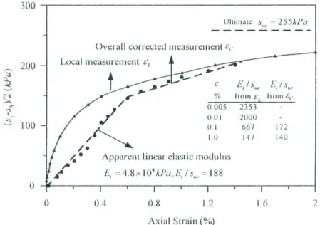
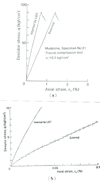
external measurement covered the behavior of high initial stiffness and non-linearity of North Sea clay at small strain.Another example is shown in Fig. 2.3 (Goto, Tatsuoka et al., 1991) in which the results of consolidated undrained compression test presented the extremely large discrepancy between external and internal measurements. And the axial strain is apparently overestimated while measured by external deformation transducers. In Fig.
2.4 presented by Diego C. F. Lo Presti et al., (1995) show how the errors in measuring
axial strains influence the Young’s modulus of Pisa clay. It can be seen that the Young’s modulus determined from external axial strains with a large-capacity LVDT are quite unreliable forε
a <0.01%.2.1.2 Local displacement transducer
As mentioned above, the external strain measurement will caused serious errors.
Therefore, how to erase the errors is an important task before investigating stress-strain behavior of soils at small strain. In past three decades, many researchers were involved in how to measure the deformation of soils more precisely. And the best one of these methods is to use the “local” displacement transducers, because all errors can be almost obviates.
2.1.2.1 Electrolytic liquid levels
Cooke and Price (1974) describe the use of electrolytic liquid levels as horizontal inclinometers for the measurement of vertical displacement around experimental piles in the field. Daramola (1978) and Costa-Filho (1980) measured relative displacement between two reference footings using local strain devices over a central length of a sample of clay and sand in laboratory tests, respectively. These devices, strictly speaking, are suitable only for very small-strain levels as a result of they are unwieldy and can suffer from jamming and damage at large strains. Although those devices are not good enough, but they create the new options of measurements and influence the
subsequent development of devices.
Burland and Symes (1982) made use of electrolytic levels to develop an axial displacement gauge, which has the resolution less than 1μm over a range of 15mm.
This gauge is the first one that can measure a wide range of axial displacement, and test results demonstrated the gauge is simple to use and applicable for wide spectrum of soils. The arrangement using an electrolytic level is shown in Fig. 2.5. The liquid level consists of an electrolyte sealed in a glass capsule. Three co-planar electrodes protrude in a line into the capsule and are partially immersed in the electrolyte. The resistance between the central electrode and the outer ones varies as the capsule is tilted. The principle can be used for measuring the changes in length.
Fig. 2.6 shows an arrangement, which converts a change in height Δh to a change
in slope Δθ. There is a spring-loaded ball hinge at C; the hinge at D rotates in two orthogonal vertical planes. Pads C and D are glued to the specimen membrane. A vertical deflection gauge, which can be used in a triaxial apparatus, is shown in Fig.2.7. The input voltage of the gauge is 5V supplied by an AC power, and the excitation
frequency is 5 kHz. The gain was adjusted to give an output sensitivity of approximately 0.4 V per degree tilt, with a scatter of ±0.002 V. The electrolyte level is sensitive to the changes in temperature, so it should be operated in the conditions, which are controlled to within ±5 . Local measurements have been measured to an ℃ accuracy of ±2μm.The typical results from an undrained test with fixed end platens on an undisturbed sample of London clay is shown in Fig. 2.8. Although the fixed end platens were used to reduce the influence of rotation of platens, the effect of sample tilts during early stages of shearing was still greatly significant. The two deflection gauges show clear evidence that this is due to sample tilt. The average of the readings from the two deflection gauges gives reasonable results that are not affected by the bedding errors.
The deflection gauge developed by Burland & Symes (1982) was improved by Jardin, et al., (1984) and carried out a series of undrained triaxial tests through making use of the gauge and measured the stress-strain behavior of geomaterials, including chalk, clay and sand at small strain. The accessories of the gauge are shown in Fig.
2.9, and the resolution of this gauge is less than 1μm.
It is beneficial that using local displacement transducer to measure the axial displacement of the sample. Nevertheless, do the readings from the transducers on the specimen represent the actual deformation of the specimen? Is it possible that relative movement occurs between the specimen and membrane? Gens (1982) used an optical technique to demonstrate that the membrane only moves in relation to the sample when large strains are developed
2.1.2.2 Hall Effect Semiconductors
Clayton and Khatrush (1986) developed a local strain device made of the semiconductor material, which make use of the Hall Effect, discovered by E.H. Hall in 1879. Hall Effect means that consider a metallic or semiconductor plate through which electrical current is flowing. If this is placed in a magnetic field where the flux lines are perpendicular both to the plate and to the current flow, the charge carries will be defected. A voltage will thus be produced across the plate in a direct normal to the current flow. This voltage is termed the Hall voltage. Hall Effect semiconductors are used widely as switches and to measure magnetic flux density.
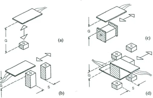
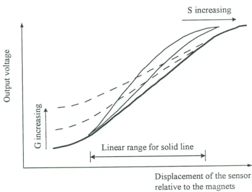
Clayton et al. (1989) described the development of Hall Effect semiconductors in geotechnical measurement. Fig. 2.10 shows the temperature compensated semiconductors manufactured by Micro-Switch have been used since 1985. Four basic configurations, shown in Fig. 2.11, of sensor and magnets have been used in geotechnical instrumentation at the University of Surrey. Fig. 2.12 shows the influence of varying both the separation S between the magnets and the gap G between the magnets and the semiconductor for a double magnet, bi-polar side-by configuration. Up to a separation S approximating to the minimum face width of the pole of the magnet, an increase in the gap results in an increase in the linear range of the device. Decreasing the gap G can increase the sensitivity of the output. Therefore, in order to get highly sensitive displacement measurement the spacing is reduced to zero, and the gap is reduced to as little as possible.
The first use of linear-output Hall Effect semiconductors was to control radial strains during K0 triaxial compression test on sand at the University of Surrey in 1983.
The prototype of the local axial strain gauge is as shown in Fig. 2.13. And Fig. 2.14 shows the design of the Hall Effect local strain gauge in Clayton and Khatrush (1986).
And this gauge is consisted of two major parts:
I. A spring-mounted pendulum that holds two bar magnets each had 3mm×3mm square cross-section area and separated by 3mm. This is suspended from an upper pad fixed to the specimen by pins, and bounded to the membrane by adhesive. The spring allows relative motion between the pendulum and the fixing pad.
II. The Hall Effect semiconductor encapsulated in epoxy resin within a brass container, which is mounted on the specimen by means of a pinned fixing pad.
In modern soil mechanics laboratory equipped with the Hall Effect semiconductor transducers, the resolution of the gauge is better than 1 µm, which is equivalent to an axial strain of less than 0.002%.
2.1.2.3 Local deformation transducer
There is another axial displacement measurement, LDT (Local Deformation Transducer), shown in Fig. 2.15 and developed by Goto, et al., (1991). Each LDT consists of a thin, hence flexible, strip of phosphor bronze and a couple of pseudo-hinged attachments. As shown in Fig. 2.15, four strain gauges, two on each side, are glued at the central part of the strip. The working principle of LDT is such that, when the specimen is deformed, the change in distance between the two attachments triggers the increase (or decrease) of the gauge strain, which in turn determines the local axial strain over the gauge length. The axial strain is the average of those measured using a couple of LTDs that are instrumented right opposite to each other (see Fig. 2.15). The resolution of the LDT is 0.6 µm, and strain levels range from 10
-6
~10-2
.2.1.2.4 Proximity transducer
The proximity transducer contains one metal target and the transducer. The working principle of the proximity transducer is such that, the deformation of sample
produced the axial displacement, and the magnetic field between the target and the transducer would be change, and this resulted in the change of the voltage. The variance of voltage represents the axial displacement of sample. Kokusho (1980) and Hird and Yung (1989) used the proximity transducer to measure axial displacement in dynamic and static triaxial tests, respectively. The resolution of the proximity transducer can reach as small as 1μm or less.
Matsumoto et al., (1998) made use of the proximity transducer (or so-called gap sensor) to measure the local strain of the sample in the triaxial tests. The arrangement of proximity transducers on sample was shown in Fig. 2.16. Generally speaking, the resolution of the proximity transducer is 0.5~1 µm. But, in recent year the researchers adopted the new LVDT, which is rather small and light, and to replace the proximity transducer. The resolution of the new LVDT is similar to the proximity transducer.
2.2 The Pore Pressure Measurement in Triaxial Test
The most common pore pressure measurement is making use of the electrical pressure transducer to measure the pressure of sample. However, the ordinary arrangement of pore pressure transducer is to connect the transducer to the bottom of the sample through nylon tube. In other words, the pore pressure measured by transducer was the pressure at the bottom of the sample, and there were lots of connectors and tubes in the path of measurement. Therefore, there are two major possible errors in measuring the pore pressure using the above method:
I. The pore pressure measured from the bottom of sample cannot represent the true pore pressure of the sample, due to the un-uniformity of the distribution of the pore pressure in soil samples, especially for clay.
II. The measurement path consisted of many connectors and nylon tubes. In the process of measuring, there might be a few air bubbles hide in connectors.
The bubbles will cause un-estimative errors in pore pressure measuring.
In order to reduce the errors and to measure the pore pressure at different positions of sample, we adopt one kind of miniature pore pressure transducer to achieve the above objects. The feature of the miniature pore pressure transducer is the very mini size, so as to place it in any position we want.
2.2.1 Standard Pore Pressure Transducer-PMP 1400
The base pore pressure measurement is making use of the pore pressure transducer PMP1400 from Druck. The range of pressure measurement is -1 bar to 4 bar. The word “standard” is meant that the transducer is commonly used in conventional triaxial test apparatus to measure the base pore water pressure. In addition to use the base pore pressure transducer, we also adopt the miniature pore water transducer to measure the pressure at the middle of sample. Therefore, the pore pressure measured at different position through two kinds of pore pressure transducer can be monitored and get comparison.
2.2.2 Miniature Pore Pressure Transducer-PDCR81
The miniature pore pressure transducer used in this research is PDCR81 from Druck. The PDCR81, shown in Fig. 2.17, consists of a 0.09-mm-thick, single-crystal, and silicon diaphragm with a fully active strain gauge bridge diffused into the surface.
A high air entry porous stone is placed in the tip of the transducer, just overlying the diaphragm. One side of the diaphragm is exposed to the atmosphere via the transducer cabling, while the other side is exposed to the pore water via the porous stone. The deformation of the diaphragm causes a change in voltage measured across the strain gauge, which is equated to pressure.
The small size of the PDCR81 allows it to be inserted easily into soil samples while causing minimal interference. The small size also leads to a quick response time since only a small amount of fluid is required to flow into or out of the device for a given change in pressure. This quick response time allows the PDCR81 to be better used for real time monitoring of pore pressure changes during testing, including dynamic events. Therefore, miniature pore pressure transducers, such as the PDCR81, are currently used in a variety of geotechnical testing applications for measuring pore water pressure.
The kit supplied comprises the following components: Druck PDCR 81 pressure transducer, 8.5mm drill and 3/8" UNF Tap, Cutter and Rubber Block, Flanged Grommet, Pair of o-rings and o-ring stretcher, Right Angle Bracket. Their purpose and installation is described below.
1. Druck PDCR 81 pressure transducer. The transducer is provided with a small ceramic tip. This is the sensing end of the transducer and is placed against the surface of the triaxial test specimen. The transducer is shrouded in heat-shrink sleeving which is connected to a bulkhead gland. The bulkhead gland is provided with an o-ring seal to seal against the outside of the triaxial cell.
2. Cutter and Rubber Block. The cutter is provided to cut a small hole in the middle of the rubber sleeve subsequently used to jacket the triaxial test specimen. Lay the rubber sleeve on a flat surface. The Rubber Block is positioned inside the rubber sleeve at the midpoint. Hold the cutting tool vertically above the block with the brass serrated end touching the rubber sleeve. Press down on the brass top of the cutter against the reaction of the rubber block while rotating the outer body of the cutter. Rotate a few times until a hole is cut in the sleeve through to the rubber block. This hole is exactly the right size to take the flanged grommet. In order to make the sleeve airtight, we used a small self-adhesive label to cover the hole while we use a suction sleeve stretcher to apply the sleeve to the test specimen.
3. Flanged Grommet. The grommet is designed to fit exactly through the hole bored in the rubber membrane jacketing the triaxial test specimen. The flange is designed to lie under the membrane against the surface of the test specimen. The grommet pokes through the membrane to receive the transducer tip.
4. Pair of o-rings and o-ring stretcher. Slide the pair of o-rings over the sensor and onto the transducer lead. Slip the o-ring stretcher over the thinner part of the transducer lead between the sensor and the bulkhead gland with the tapered end away from the sensor. Slide the two o-rings onto the stretcher from the tapered end. Push the sensor into the grommet so that the ceramic tip is against the surface of the test specimen. Slide the o-ring stretcher along the cable, over the sensor, and up against the test specimen. Roll the o-rings off so that the grommet grips the sensor and holds it in place against the surface of the test specimen.
5. Right Angle Bracket. Close to the sensor, slip one end of the Right Angle Bracket onto the cable. Then bend the cable gently around into a right angle and slip the cable into the other end of the Right Angle Bracket. This leads the cable nicely away from the wall of the triaxial cell and down to the bulkhead gland.
The advantage of using midheight pore pressure transducer was point out by Sheahan, Ladd and Germaine (1996). The response times of base and midheight pore pressure devices were measured during B-value checks. The midheight device response fully (i.e. a B-value of at least 95% is measured) within 5-7 seconds and the base device within 45-60 seconds.
2.3 Load and Temperature Measurement in Triaxial Test System 2.3.1 Load Cell
The load cell is placed in the triaxial cell and fix with the upper shaft, hence it must be watertight. Because there will be cell pressure in the triaxial cell, therefore the load cell must have the ability to resist pressure, which has the maximum value of
5 2
cm
kg during the test. The load cell, Models 31, chosen for this test system is the
product of Sensotec. Models 31, the precision miniature load cells measure both tension and compression load, and the load capacity is 500 lbs in our test system.
Models 31’s welded, stainless steel construction is design to eliminate or reduce to a minimum, the effects of off-axis loads.
2.3.2 Temperature transducer
The variation in temperature is monitored during test performed through the temperature transducer, so as to avoid the sharp change in temperature and protect all measurement transducers from damages. The temperature transducer used in this test system is the TK-F from TML (Japan). And the full scale of TK-F is -20℃ to 80℃.
2.4 The Calibration of All Sensors
The detailed information of whole measurement transducer in the triaxial test system is shown in Tab. 2.1. In the table, the manufacturer, sensor type, the total
measured range, excitation voltage and output voltage (before and after amplification) are shown. Usually, the sensor was calibrated in factory as soon as manufactured. But because of the different in environmental between manufacturer and Taiwan, so it is necessary to do calibration again in our laboratory.
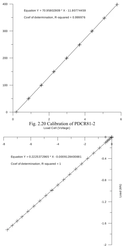
2.4.1 The calibration for pore pressure transducers
As shown in Tab. 2.1, there were three pore water pressure transducer in the triaxial test system, two miniature pore pressure transducer PDCR81 and one standard pore pressure transducer PMP1400. Two reference pore pressure transducers, one is the cell pressure transducer from GDS and another is from the CMC CO., LTD, were used in the calibration mentioned above. The results of calibration are shown in Fig.
2.18, 2.19 and 2.20.
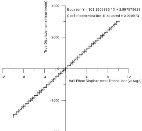
2.4.2 The calibration for load cell and temperature transducer
The calibration for load cell is to put dead load on load cell either tension or compression, since the linearity of the load cell is the same under tension or compression. The resolution of the weight used to represent the dead load is 1 g. Fig.
2.21 shows the result of the calibration for load cell.
It is difficult to calibrate the temperature transducer, TK-F from TML, in our laboratory because of the lack of the reference temperature. Therefore, the calibration is performed by using a digital thermometer, TES1310 from TES, from CMC CO., LTD. The certificate of calibration of TES1310 is shown in Fig. 2.22. And the result of the calibration for TK-F is shown in Fig. 2.23.
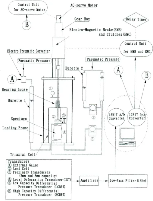
2.4.3 The calibration for Hall Effect semiconductor transducers
A special designed rig was adopted in the calibration for Hall Effect local strain measurements. The calibration rig, shown in Fig. 2.24, consisted of a precision frame and a digital micrometer head with high resolution of 1µm and high accuracy of ± 2µm. The digital micrometer head, 350-251, is from Mitutoyo. The data sheets of calibration for Hall Effect local strain transducers are shown in Fig. 2.25 and 2.26.
Tab. 2.1 Detailed information of all transducers
Small-Strain Triaxial Anisotropy Testing System
channel manufacturer type excitation voltage output voltage before output voltage after the total measured function
amplification amplification range
CH0 Sensotec Model 31 10Vdc -20mVdc~+20mVdc -10Vdc~+10Vdc -500 lb~+500 lb Load Cell
CH1 Druck PMP 1400 10Vdc 0~+5Vdc -2.5Vdc~+10Vdc -1 barg~+4 barg Pressure Transducer
CH2 Druck PDCR 81 5Vdc 0~+81.9mVdc 0~+10Vdc 0~7 barg Mid-plane Pore Pressure
Transducer 1
CH3 Druck PDCR 81 5Vdc 0~+80.96mVDc 0~+10Vdc 0~7 barg Mid-plane Pore Pressure
Transducer 2
CH4 Hall Effect 50 532 10Vdc +3.5Vdc~+6.5Vdc -10Vdc~+10Vdc -3 mm~+3 mm Local Deformation Transducer
Axial 1
CH5 Hall Effect 50 533 10Vdc +3.5Vdc~+6.5Vdc -10Vdc~+10Vdc -3 mm~+3 mm Local Deformation Transducer
Axial 2
CH6 Hall Effect 76 565 10Vdc +3.5Vdc~+6.5Vdc -10Vdc~+10Vdc -3 mm~+3 mm Local Deformation Transducer
Radial
CH7 TML TK-F 5Vdc -6.985mVdc~+27.94mVdc -2.5Vdc~+10Vdc -20℃~+80℃ Temperature Transducer
Fig. 2.1 The errors produced in conventional triaxial testing apparatus.
Fig. 2.2 the result of comparison of using external and internal measurement (Jardin, et al., 1984)
Fig. 2.3 Stress-strain relationship of a sedimentary soft rock in drained triaxial compression test; (a) Maximum scale for
ε
a equal to 3% (b) 0.1% (Goto, Tatsuokaet al., 1991)
Fig. 2.4 Young’s modulus of k
0
consolidated Pisa clay specimen (Diego C. F. Lo Presti et al., 1995)Fig. 2.5 Arrangement of an electrolytic level (Burland and Symes, 1982)
Fig. 2.6 Arrangement of an electrolytic level to measure axial displacement (Burland and Symes, 1982)
Fig. 2.7 A vertical deflection gauge using electrolytic level (Burland and Symes, 1982)
Fig. 2.8 Comparison of axial displacement between local measurement and external measurement (Burland and Symes, 1982)
Fig 2.9 Arrangement of the electrolytic gauge (Jardin, et al., 1984)
Fig. 2.10 Photograph of a Hall Effect transducer (Clayton, et al., 1989)
Fig 2.11 Basic configurations of sensor/magnet systems: (a) single magnet, head-on, (b) double magnet, bi-polar slide-by, (c) signal magnet, bi-polar slide-by, with pole
pieces, and (d) tandem double magnet bi-polar slide-by (Clayton, et al., 1989)
Fig. 2.12 Effect of varying magnet gap and spacing on output from a double magnet slide-by configuration (Clayton, et al., 1989)
Fig 2.13 Prototype of local axial strain gauge (Clayton and Khatrush, 1986)
Fig. 2.14 Design of the Hall Effect local strain gauge (Clayton and Khatrush, 1986)
Fig. 2.15 Set-up of local deformation transducer (LDT) (Goto, et al., 1991)
Fig. 2.16Arrangement of proximity transducers in the triaxial cell (Matsuomoto et al., 1998)
Fig. 2.17 The miniature pore pressure transducer PDCR81 (after Kutter et al., 1990)
0 4 8 12 0
100 200 300 400
Equ atio n Y = 39 .5 51 79 34 9 * X - 2.88 24 31 97 5 Co ef of d etermina tion , R-squ ared = 0 .999 99 4
Fig. 2.18 Calibration of Druck PMP1400
0 2 4 6
0 100 200 300 400
Equ atio n Y = 6 8.60 827 80 3 * X + 1.33 646 85 88 Co ef o f de te rmin atio n, R-sq ua red = 0 .9 99 97
Fig. 2.19 Calibration of PDCR81-1
0 2 4 6 0
100 200 300 400
Eq ua tion Y = 70 .9 58 028 09 * X - 11 .8 077 44 59 Co ef of d etermina tion , R-squ ared = 0.999 97 6
Fig. 2.20 Calibration of PDCR81-2
-8 -6 -4 -2 0
Lo ad Cell (Volta ge )
-2 -1.6 -1.2 -0.8 -0.4 0
Lo a d ( k N )
Eq ua tion Y = 0.22 25 37 296 5 * X - 0 .0 00 91 284 00 88 1 Co ef of d etermina tion , R-squ ared = 1
Fig. 2.21 Calibration of load cell
Fig. 2.22 The certificate of calibration of TES1310
3 4 5 6 7 25
30 35 40 45 50
Equ ation Y = 7 .3 29 20 71 24 * X + 3.01 35 85 75 Co ef o f de te rmin ation, R-squa red = 0 .9 99 89 7
Fig. 2.23 Calibration of temperature transducer TK-F
Fig. 2.24 (a) Calibration rig for Hall Effect sensors (bird-view)
Fig. 2.24 (b) Calibration rig for Hall Effect sensors (side-view)
-12 -8 -4 0 4 8 1 2
Ha ll Effect Disp la ce ment Tran sd uce r (vo ltag e)
-4000 -2000 0 2000 4000
T ru e D is p la c e m e n t (m ic ro -m et er)
Eq uation Y = 310 .653 48 9 * X + 4.60 42 361 03 Co ef of determination, R-squared = 0.9998
Fig. 2.25 Calibration of Hall Effect displacement transducer-axial 2
-12 -8 -4 0 4 8 1 2 Ha ll Effect Disp la ce ment Tran sd uce r (vo ltag e)
-4000 -2000 0 2000 4000
T ru e D is p la c e m e n t (m ic ro -m et er)
Equa tio n Y = 30 1.19 05 88 3 * X + 2.99 757 96 29 Coe f of determina tio n, R-sq uare d = 0.99 99 73
Fig. 2.26 Calibration of Hall Effect displacement transducer-radial
Chapter 3
Pressure Controller and Loading System 3.1 Pressure Control System
The pressure control system is considerably important and essential for all routine laboratory tests, especially in stress path method and k
0
consolidation stage of triaxial test. There were several different mode of providing pressure, the tradition laboratory pressure source such as mercury column, compressed air, pumped oil, and dead load device. And the digital pressure controller is a constant pressure source which can replace the tradition one. The objective of design for the digital pressure controller is to reach the target pressure gave by user steadily and smoothly.3.1.1 Mechanical component
The digital pressure controller can be cut into three major components, which are motor, transducer and control circuit. The configuration of the digital pressure controller is shown in Fig. 3.1. The part of motor includes a stepping motor, gearbox and ball screw. The stepping motor receives the pulses converted from the ADC chip, and rotates the ball screw to push a piston moving in the cylinder through the gearbox.
Accordingly, liquid in the cylinder is pressurized and displaced, and then the volume change can be measured by counting the steps of the incremental motor.
The second part is transducer, used in the measurement of pressure and send signals to ADC chip. The transducer is PMP1400 from Druck, and the range is 0 bar to 10 bar. As shown in Fig. 3.1, the transducer is in the special position below the pressure out valve. Therefore the air bubbles will no logger stay in the transducer.
The last part of the digital pressure controller is the control circuit. It consisted of the kernel--ADC chip, liquid crystal display (LCD), touch panel and a few circuits.
The ADC chip has the function of converting the analog input signals to digital signals, and then the digital signals are displayed on the LCD. The contents shown on the LCD include the pressure, volume and system states. The signals converted from ADC chip also send into computer through RS-232. It means that the digital pressure controller can be read and controlled directly from a computer.
3.1.2 Resolution, functions and operations
The digital pressure controller can not only measure and control pressure but also volume simultaneously. But the resolution and accuracy does really satisfy the needs of special stages when performing triaxial tests? First, the analog signal of pore pressure transducer is acquired by a 16-bit DAQ card, so the resolution is 0.015 kPa.
The NLH (Non-linearity & Hysteresis) of the PMP1400 is ±0.25% max, and it is obviously that the resolution of 0.015 kPa is good enough for the pressure sensor under the errors of the NHL. The resolution of reading and control on volume change is 1 mm
3
or better, namely the volume strain can be read as small as 0.00017%.The detailed interpretation of the LCD display on control panel is as following:
1. It shows the readings of water pressure continuously, which is not via the computer. The signals of water pressure transducer was not only received and shown by ADC chip, but also on computer testing program. In order to protect the transducer, the stepping motor should be terminated when the pressure is exceeding the set limit regardless of under which control mode.
2. The volume change is shown in the LCD as well as the pressure readings, and it is not via the computer either. The calculation of the volume change is the result of the distance of stepping motor moved multiply the cross area of the cylinder. The symbol “+” represents the emptying water (means the volume in cylinder is decrease), and the symbol “-” indicates that the controller is filling water into the cylinder (i.e. the volume change of the cylinder is positive).
3. The LCD also displayed the state of the digital pressure controller. For example, it will show “Caution: Pressure” when water pressure exceeds the upper or lower limit, and show “Caution: Volume” when stepping motor is approaching the limit switch. Furthermore, the LCD will show the motion of the control system, such as “Filling water” when press the Fill button and so on.
The figure of the control panel of the digital pressure controller is shown in Fig.
3.2. There are two ways to control the digital pressure controller, the first one is
through the computer testing program and another is using the control panel. When the digital pressure controller is controlled by computer testing program, it can not accept the manual input commands from the control panel unless operator press
“Shift” and “Reset” at the same time.
The functions of each button on control panel are going into details as following:
“Enter”—to start to execute the motions inputted by users.
“Stop”—to stop all motions of the digital pressure controller manually.
“Reset”—to clear values, settings on LCD, and turn the controller to manual control when press “Shift” and “Reset” simultaneously.
“Shift”—to execute the sub-function of the button marked sub-functionally if pressing the “Shift” and any one of the sub-functional button at the same time.
“Empty” and “Fill”—to empty the liquid (normally deaerated water) from the cylinder or fill up the cylinder with liquid.
“1 & (P-target)”— two functions were set in this button, the first is to input the numeral “1”, and the sub-function is to set the target pressure needed in performing test.
“2 & (P-zero)”—to input the mineral “2”, and the controller will set the current pressure as zero point when press this button and “Shift” together.
“4 & (V-target)”—the functions of this button are to input the numeral “4”
and the target volume of liquid in cylinder.
“5 & (V-zero)”—In addition to input the numeral “5”, the sub-function is to set the volume as reference zero point.
Numeral buttons “3, 6, 7, 8, 9, and 0” are purely to input the numeral marked.
3.2 Loading System
Typically, triaxial tests require independent control of the axial stress and the cell pressure, especially for stress path tests. In this triaxial test system, the cell pressure was provided by independent controller introduced in section 3.1. The axial or deviator stress may be supplied either mechanically or by fluid pressure, and the two commonly available systems are illustrated in Fig. 3.3. Fig. 3.3(a) illustrates the conventional triaxial arrangement in which a triaxial cell is contained in a loading frame and a ram loads the top of the sample as the cell is raised by mechanical drive.
Fig. 3.3(b) illustrates a hydraulic triaxial cell in which the bottom platen is raised by fluid pressure acting in lower chamber. The represent of the two loading system will be introduced in detail below.
3.2.1 The Bishop & Wesley 1975
The Bishop and Wesley hydraulic triaxial apparatus is shown in Fig. 3.4. A cross-sectional scale view is shown in Fig. 3.5. The upper part of this system is similar to a conventional triaxial cell except that the axial load in axial compression test is applied by moving the sample pedestal upwards from below and pushing the top cap against a stationary load cell, which records the load.
The pedestal is mounted at the top of the loading ram, at the bottom end of which is a piston and pressure chamber. Bellofram rolling seals are used to retain the cell fluid and the ram travels up and down in a “Rotolin” linear bearing. The axial load is applied to the sample by increasing the pressure in the bottom pressure chamber.
The loading ram has a cross-arm attached to it which moves up and down in wide slots in a “spacer” which connects the bearing house to lower pressure chamber.
The cross-arm supports two vertical rods which pass through clearance holes in the cell base and deflect the dial gauges (or displacement transducers) mounted on the top of the cell. Then these gauges records the movement of the arm from which the axial strain in the sample is determined. Only one vertical rod would actually be sufficient but two were used to keep the arm balanced and to enable both a dial gauge and transducer to be mounted at the same time.
The drainage and pore pressure leads from the sample pedestal are taken down the center of the load ram and out through slots in the spacer. Provision is made for
drainage leads from the top cap should these be required.
A lot of alternative arrangements were considered before getting to this design. It may seem more logical to load the sample from above as in conventional test, but the arrangement with the load applied from below has several advantages. It is quite simple to set up the sample, as in a conventional apparatus, but no corrections are required for load ram weight. The upper part of the cell which is removed for mounting or dismantling the sample remains light in weight and easy to handle. The weight of the ram acts against the lower Bellofram seal and maintains a positive pressure in the pressure chamber so that there is no danger of damaging the rolling seal by turning it inside out.
The use of two Bellofram seals perhaps required some explanation since it would be possible to use only one seal to separate the cell fluid from the pressure chamber fluid. The two seals have the following advantages. First, strain measurement can be made externally by means of the cross-arm arrangement attached to the ram between the seals. Second, extension tests (i.e. tests in which the horizontal stress is greater than the vertical stress) are possible as the pressure in the pressure chamber can be made less than the cell pressure. Third, the linear bearing is not submerged in cell or loading chamber fluid so that the use of oil to protect the Rotolin bearing in either of these is unnecessary.
Extension tests are made possible by attaching a small device to the load cell which, on partial rotation, connects it to the sample top cap. Extension tests with plain end caps are however only possible if a cell pressure is applied, the magnitude of which is function of the strength of the sample.
It should be noted that the apparatus is self-contained; it requires no loading frame and is quite portable. It is equally well suited to both stress controlled and strain controlled loading. To operate the cell auxiliary equipment is required in the form of two controllable pressure sources (for controlled stress tests) or a controlled pressure source and a constant rate of flow source (for axial-strain controlled test).
The test may be run either undrained or consolidated undrained with or without pore pressure measurement; or drained, either to atmospheric pressure or against a
constant or varied back pressure, the last two cases requiring a third pressure control unit.
3.2.2 The modified commercial triaxial testing system from Italy
The modified triaxial testing system was introduced by Diego C. F. Presti et al.
1995. The mechanical modification of this triaxial apparatus concerned cell structure and loading system. Three tie rods connecting the base plate to the top plate were located inside the Lucite pressure cell, thus substituting the eight external tie rods (Fig.
3.6). This modification has been suggested by many researchers (Alva-Hurtado et al.
1980; Berre 1982; Ladd and Dutko 1985; Tatsuoka 1988; and Baldi et al. 1988). The Extension caps which usually allow horizontal stresses greater than vertical stresses (Menzies 1988) is unnecessary because the top cap is rigidly connected with the upper cell plate. Moreover, it makes specimen setting easier and strongly improves the alignment between the specimen and loading rod. The new pieces were made of stainless steel.
The modified loading system is shown in Fig. 3.6a, while the original one is depicted in Fig. 3.6b. The most relevant modification is the reduction of the loading rod diameter from 16 to about 7 cm, which is more or less the diameter of the standard specimen. An advantage of this modification is that the lower chamber pressure provides the vertical stress, while the cell pressure provides the horizontal stress independently from each other.
As far as the actuator resolution is concerned, it should be noted that the DC operates under both stress and strain rate control. The minimum pressure increment and minimum volume change that the DC can deliver are equal to 1 kPa (0.5 kPa for the more recent version of DC) and 1 mm
3
, respectively. Therefore, with the new geometry of the loading piston and without considering the friction between rod and ball bearing, the minimum stress and minimum axial strain that the actuator can deliver, in the case of a standard specimen, are respectively equal to:1. 1 kPa (under stress rate control).
2. 0.0002% (under strain rate control).
3.2.3 The triaxial testing system from University of Tokyo
The modification was made to an existing triaxial testing apparatus by Tatsuoka ea al. (1999) to more accurately evaluate the stress-strain behavior of geomaterials for wide ranges of strain and strain rate. The device is now driven by an a-c servo motor, allowing for changing the strain rate about three orders of magnitude without any intermission in each test. And the modification of loading system will be introduced in detail in the following paragraph.
The basic components of the system shown in Fig. 3.7 are a triaxial cell, a unique mechanical axial loading system, a pneumatic cell pressure system, and several transducers, connected throughout D/A and A/D cards to a microcomputer that controls the tests and records the data (Tatsuoka 1988). The driving motor of the axial loading system is shown in Fig. 3.8.
In the modified system shown in Figs. 3.7 and 3.8, the loading device is driven by an a-c analog motor that is connected though a series of speed-reduction gear boxes to the axial loading shaft. The previously adopted conventional analog motor has been replaced with an a-c servo-analog motor. This relatively simple and economic system allows one to:
1. To maintain an essentially constant strain rate.
2. To execute very small unload –reload cycles with an axial strain amplitude of the order of 0.001% or less without a noticeable time lag when reversing the loading direction.
The loading device was designed to automatically switch the motor on or off and select the upward or downward direction of the movement of the axial loading shaft through a personal computer and a D/A card. By means of a simple control loop, it is then possible to maintain an essentially constant deviator stress, even in a transient stage like a consolidation process or a creep test, by setting the prescribed axial displacement rate to be higher than that at which the specimen would tend to axially deform under the imposed stress state. More over, by using the axial loading device and a pneumatic cell pressure system, the stress path can be controlled rather accurately by adjusting the air pressure acting on the cell water (Ampadu and
Tatsuoka 1989)
The new loading device is now driven by an a-c servo motor equipped with a digital servo driver. The improvement in performance is due to mainly to feedback system of the a-c servo motor, which is schematically illustrates in Fig. 3.9. An optical encoder is attached to the motor body in order to measure: (a) the position and (b) the rotation rate of the rotor by means of a set of electro-optic units. The typical torque capacity of the a-c servo motor is compared to that of the previously used motor in Figs. 3.10a and 3.10b. And for the servo motor, the rotation rate can be varied between 0 to 3000 rpm by keeping almost the same torque capacity.
3.2.4 The loading system of small-strain triaxial testing system in NTUST
According to the modification of loading system mentioned above, the tendency to apply axial load is making use of motor and transmissions rather than using pressure. The reason of modifying the loading system by using mechanical device, i.e.motors and gears, is the high precision of axial displacement and variable strain rate under strain controlled. Therefore, in this triaxial testing system designed in NTUST, the servo motor was adopted in modifying the loading system. And the servo motor used in our loading system is totally different from which is used in the testing apparatus modified by Tatsuoka, because of the transmission was modified in this system also. The objects of modifications in this triaxial testing system are listed below:
1. Providing constant output torque under any strain rates (i.e. the rotation rate of motor).
2. Reducing the errors from the transmission, especially the backlash in ball screw and motor may be 10~100 times greater than single axial displaced increment.
3. High resolution and precision of axial displacement in any testing stage and any stress level.
3.2.4.1 The determination of the maximum torque capacity of motor
The first step of design the loading system is to decide for the torque capacity ofservo motor. The size of specimen is 71 mm in diameter and 150 mm in height, thus the cross area can be calculated. The axial load on pedestal is dependent on the stress state of the sample during testing process and the maximum stress in each testing stage was estimated:
During saturation stage, the cell pressure and the back pressure are 196 and 191 kPa, respectively.
During k
0
consolidated stage, because theγ
t of Taipei silty clay is less than 1.95 3m
t and the sampled depth is smaller than 30 m usually, therefore the maximum axial consolidated stress is 280 kPa.
The normalization strength
( )
' ' 3 ' 1
2
σvc σ σ−
of Taipei silty clay is approximately 0.3 (H.T. Liu2004). Therefore, the increment of axial stress is 0.6 times of the effective vertical consolidated stress, and maximum of which is 168 kPa.
The sum of the stresses mentioned above is 640 kPa, and the axial force corresponding to this stress is 251 kg. It means that the servo motor must provide the thrust of 251 kg after transmitted by ball screw. Considering the safety factor, the maximum thrust was raised to 400 kg for designing the loading system. The conversion from axial load to the torque capacity of motor is making use of the experiential equation shown in Eq. 3.1 from mechanics.
Torque= N×M Eq. (3.1)
N: axial load; M=Pitch2
π
The axial load N is 400 kg, i.e. 3924 N in this system, and the pitch of the ball screw is 5 mm. The torque capacity calculated from Eq. 3.1 multiplied the safety factor, and the final result is 18.735 N-m.