自適應布穀鳥過濾器: 避免非必要的硬碟操作

國立臺灣大學電機資訊學院電機工程學系 碩士論文

Graduate Institute of Electrical Engineering College of Electrical Engineering and Computer Science

National Taiwan University Master Thesis

自適應布穀鳥過濾器: 避免非必要的硬碟操作 Adaptive Cuckoo Filters: Avoiding Trips to Disk

吳佳倫 Chia-Lun Wu

指導教授：陳銘憲 博士 Advisor: Ming-Syan Chen, Ph.D.

中華民國 105 年 7 月 July 2016

Acknowledgements

This work is supported by ITRI (Industrial Technology Research Institute) in Taiwan. I grate- fully acknowledge the colleagues in ITRI: Yu-Lun Chen, Hung-Hsuan Lin, Chen-Ting Chang, Tzi- Cker Chiueh. Through the active discussion with them during the weekly meetings in the early morn- ing and receiving their valuable feedbacks, I got many inspirations to further improve my work.

Besides, I would like to thank my advisor, Prof. Ming-Syan Chen for his support, guidance, and encouragement. He has inspired me not only the research strength but also the direction of my life plan. I really appreciate his trust on me.

Also, I need to give my great thanks to my fellow mates in Network Database Laboratory for all the invaluable discussion we had. It’s my pleasure to learn and grow (no shrink) with them over the past 2 years and I’ll cherish these valuable memories.

Last but not least, thanks to my family for their endless spiritual support that always give me energy to overcome the obstacles I’ve ever encountered.

中文摘要

布隆過濾器已經長時間地在各個領域被用來做快速的近似集合成員測試因為它具有簡 單但有效的設計。近年來，一種新型態的過濾器 – 布穀鳥過濾器被提出，布穀鳥過濾器支援 刪除元素的動作，而且不管在時間上或空間上都比標準的布隆過濾器以及能支援刪除動作的 布隆過濾器變形在實務上有更好的表現。然而，在 OLTP 資料庫的使用情境中，物件的存取 分佈通常是高度不均勻的，也就是某些物件被存取的比其他物件多很多，而在這樣的存取模 式中會讓傳統的布隆過濾器以及布穀鳥過濾器無法達到它們理論上該有的偽陽性比率，因為 他們都是在假定物件的存取分佈是均勻的情況所設計。

在這篇論文中，我們基於傳統的布穀鳥過濾器而設計了一種新的資料結構 – 自適應性 布穀鳥過濾器。我們採用一系列小的布穀鳥過濾器，而在存取分佈不均勻時動態調整部分布 穀鳥過濾器的大小以達到比傳統布穀鳥過濾器更低的偽陽性比率。這篇論文展示詳盡的實驗 結果，包含 ACF 的空間使用，偽陽性比率與速度效能。此外，我們也介紹 ACF 如何被應用 在一個物聯網資料庫引擎中並且在真實的資料存取模式中有很好的表現。

ABSTRACT

Bloom filters have been used for fast approximate set membership tests in various areas in a long history because of its compact and simple design. Recently, a newly proposed data structure - Cuckoo filter supports dynamic deletion of elements and has practically better performance in both time and space than Bloom filter and its variants. However, in the scenario of OLTP databases, the access workload is often skewed and will make both Bloom filter and Cuckoo filter fail to achieve their target false positive rate which is calculated in the assumption that the workload is uniform distributed.

In this thesis, we present a new data structure called Adaptive Cuckoo Filters (ACF) which can exploit the skewed access pattern and dynamically adjust the size of a list of cuckoo filters to achieve smaller false positive rate than a single cuckoo filter. This thesis also shows the results of compre- hensive experiments covering space, precision and speed of ACF. Furthermore, we show how ACF can be applied to an IoT database engine and achieve better performance in real workload.

CONTENTS

口試委員會審定書 ... i

Acknowledgements ... ii

中文摘要 ... iii

ABSTRACT ... iv

CONTENTS ... v

LIST OF FIGURES ... vi

Chapter 1 Introduction ... 1

Chapter 2 Application Background ... 3

Chapter 3 Related Work ... 4

3.1 Bloom Filters and Variants ... 4

3.2 Cuckoo Filter ... 5

3.3 Split Bloom Filters ... 6

Chapter 4 Adaptive Cuckoo Filters ... 8

4.1 Overview ... 8

4.2 Data Structure ... 10

4.3 Operations ... 11

4.4 Adaptive Strategy ... 14

4.5 Negative Cache ... 17

Chapter 5 Experiments ... 18

5.1 Benchmark Environment ... 18

5.2 Software/Hardware Settings ... 19

5.3 Experiment 1: False Positives ... 20

5.4 Experiment 2: Speed ... 22

5.5 Experiment 3: Grow/Shrink Buckets ... 23

5.6 Experiment 4: Grow Threshold ... 25

5.7 Experiment 5: Negative Cache ... 27

5.8 Experiment 6: Combinations ... 29

Chapter 6 Conclusion ... 30

Bibliography ... 31

LIST OF FIGURES

Figure 1:

... 2

Figure 2:

... 9

Figure 3:

... 10

Figure 4:

... 21

Figure 5:

... 22

Figure 6:

... 22

Figure 7:

... 23

Figure 8:

... 24

Figure 9:

... 26

Figure 10:

... 28

Figure 11:

... 29

Chapter 1

Introduction

In many applications, such as databases, web caches, routers, and storage system, an access filter is used to determine if a queried item is in a (usually large) set to avoid doing unnecessary and rela- tively expensive operations (ex: disk, network). This kind of access filter is a probabilistic data struc- ture that can do approximate set membership tests of small false positive rate but no false negatives, and it is usually put in memory or cache to achieve fast speed.

The most well-known and widely adopted access filter is Bloom filter [4]. Bloom filter is a compact data structure which can represent an item with 1.44 log₂(1/𝜖) with false positive rate 𝜖, close to information-theoretic minimum log₂(1/𝜖). It has been used to improve read throughput in Apache Cassandra database [2],

to improve processing joins in distributed systems [10], and to speed up Squid cache where the Bloom filters are referred to as cache digests [1]. Recently, a new data structure called cuckoo filter [6] has practically higher performance than Bloom filter and the Bloom filter variants. Furthermore, it sup- ports deletion, which is not allowed in traditional Bloom filter.

However, both Bloom filter and cuckoo filter are designed for uniformly distributed queries.

When the workload is skewed, such as OLTP workload, they will not have optimal performance. In this thesis, we aim to optimize the access filter in the skewed workload. For example, in Microsoft’s project Siberia [3], a framework for managing cold data in the Microsoft Hekaton main-memory database engine [7] which is targeted for OLTP workload, it uses a new form of Bloom filters called Split Bloom filters optimized for skewed workload to reduce unnecessary cold storage access.

The main contribution of this thesis is the description of a new type of filter called Adaptive

Cuckoo Filter (ACF) which is based on cuckoo filter. Concisely, an ACF is an array of cuckoo filters, so it has all the good properties of cuckoo filter plus the ability to adapt to skewed workload by adjusting the number of buckets or size of fingerprint of some cuckoo filters dynamically. Although the added complexity to be adaptive makes ACF has a little bit slower query speed than cuckoo filter, but it pays off because it can lower the false positive rate remarkably, saving many unnecessary ex- pensive disk accesses.

This thesis summarized the results of experiments conducted with ACF thereby varying the query distribution. We compare ACF with cuckoo filter, Bloom filter and split Bloom filters which is the state-of-the-art type of filter targeting on skewed workload too. The results show that ACF is robust and fast. Furthermore, it can adapt to skewed workload effectively and has the lowest false positives.

The thesis is organized as follows: Chapter 2 gives an overview of the BUSC database engine and the role of ACF in this system. Chapter 3 describes our main related works. Chapter 4 describes the data structure of ACF and how it can adapt to skewed workload. Chapter 5 shows the results of experiments. Chapter 6 is the conclusion of our work.

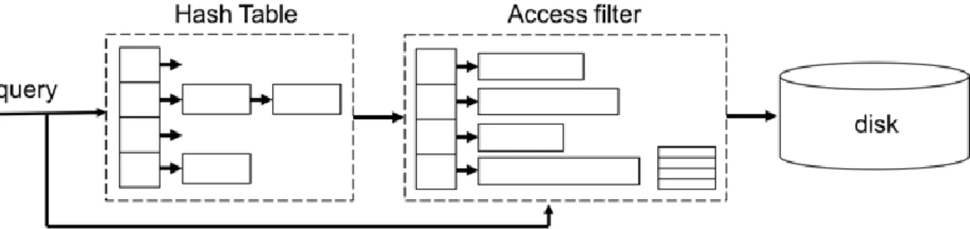
Figure 1. Simplified Query Flow of BUSC

Chapter 2

Application Background

To demonstrate the usefulness of ACF, this chapter shows how ACF is used in Project BUSC at ITRI. BUSC is a database engine targeted to handle sensor data in IoT application. The workload is analogue of OLTP. There are large number of small sensor data records coming in and occasional on-demand random reads. The working set will be more than the memory can hold, so it’s still needed to persist data to disk eventually. The main part of BUSC is an in-memory hash table storing the hot data that is frequently accessed and has particularly low latency requirements. It adopts a technique called batching updates with sequential commit (BUSC) [8] which leverages the advantage of sequen- tial write of disk and minimizes the performance overhead of the random writes. It’ll periodically bring dirty buckets in the hash table to disk.

Supposing BUSC stores IoT time-series data and each key correspond to multiple object with different timestamps, some objects may be in the memory and some may be in the disk. Thus, we need an in-memory access filter representing the items in the disk. On every query, as shown in Figure 1, both of the hash table and the access filter will be checked and if the access filter returns true, then the trips to disk will be processed.

Our goal is to design an access filter to avoid unnecessary and costly trips to disk and able to adapt to skewed query workload and meet the following requirements: (1) low false positive rate (2) fast query speed (3) small average bits per item in the filter.

Chapter 3

Related Work

3.1 Bloom Filters and Variants

Bloom filter was introduced in 1970 by Burton H. Bloom [4]. A Bloom filter consists of a bit array with all bits initially set to “0” and k hash functions. To insert an item into the filter, it hashes the item to k positions in the bit array by k hash functions, and sets these k bits to “1”. For lookup, it reads k corresponding bits in the array: if all the bits are set to “1”, the query returns true; otherwise it returns false. It will only cause false positives (answer the item in the set but it isn’t) but no false negatives (answer the item not in the set but it is actually in it). The false positive rate of Bloom filter can be approximately by

𝑓𝑝𝑝 = (1 − 𝑒

)

(1)

where k is the number of hash functions, n the number of distinct keys in the filter, and m is the number of bits of the bit array.

There are numerous extensions of the standard Bloom filter having been proposed to optimize in some scenarios or to improve Bloom filter in space or performance. For example, Counting Bloom filters [11] extend Bloom filter to allow deletions but has 4 × more space than a standard Bloom filter. Blocked Bloom filters [9] provide better spatial locality on lookup by using an array of small Bloom filters that each can fit in one CPU cache line. Weighted Bloom filters [5] use different number of hash functions for each key depending on the key’s lookup frequency to optimize the false positive rate in skewed workload. Conscious Bloom filters [13] use a (2 + 𝜖)-Approximation algorithm to decide how many hashes to use.

Both weighted Bloom filters and conscious Bloom filters try to optimize for skewed workloads.

However, because they assume that the lookup frequency of items is known in prior, they cannot adjust to changes in the access skew dynamically and they don’t allow deletions as well.

3.2 Cuckoo Filter

Cuckoo filter is a newly proposed data structure which supports deletion and outperforms the standard Bloom filter and its variants that support deletion in false positive rate and performance [6].

The structure of cuckoo filter is literally a hash table with multiple entries of a bucket and each entry store the fingerprint of an item.

Cuckoo filter is an extension of cuckoo hash table which is based on cuckoo hashing, a family of hashing techniques. In cuckoo hashing, each key has only two possible locations to be stored, which are determined by two independent hash functions. Thus, processing lookup query is simple:

just check the two cells and test if the query key is in the cells.

Inserting a key into the cuckoo hash table is more complicated. If one of the two cells for the key is empty, the key can be stored into it directly. Otherwise, one of the keys of the two cells will be kicked off and re-inserted into its alternative location. It’s possible that the kicked-off key might kick off another key. Therefore, the insertion operation is an iterative process that will either terminate with all keys stored in one of their two cells, or it may fail (usually determined as the number of kick- off is higher than 500 times) and incur the rebuild process of the whole data structure.

Instead of storing the key-value pair into the hash table, a cuckoo filter stores a small fingerprint for each element in a set. Like a cuckoo hash table, a cuckoo filter may sometimes move the finger- prints to their alternative location for the key. Therefore, it needs to determine the alternative location for a fingerprint from the fingerprint alone by utilizing a technique called partial-key cuckoo hashing.

Using this technique, we can derive a fingerprint’s alternative index by a bitwise exclusive or opera- tion given the fingerprint and its index in the table no matter the fingerprint is in which of its possible two locations, because exclusive or is an involution. However, the exclusive or operation will make

the number of buckets N in the cuckoo filter be power of two which is not good if we want to adjust the size of cuckoo filter in a fine-grained way.

The false positive rate of cuckoo filter is shown as follows where n is the number in the filter, b the number of buckets and fp is the fingerprint size in bits.

𝑓𝑝𝑝 =

𝑏×2^𝑓𝑝

(2)

Cuckoo filters improve upon Bloom filters in three ways: (1) support for deleting items dynam- ically; (2) better lookup performance; and (3) better space efficiency for applications requiring low false positive rates (𝜖 < 3%). A cuckoo filter stores the fingerprints of a set of items based on cuckoo hashing, thus achieve high space occupancy. Because of these advantages, we choose cuckoo filter as our foundation.

3.3 Split Bloom Filters

Split Bloom filters is proposed in [12] and is used as the access filter in the Siberia [3], a frame-

work for managing cold data in the Microsoft Hekaton main-memory OLTP database engine, to avoid unnecessary trip to the cold store. It is specifically designed to exploit the access skew to achieve lower false positive rate than standard Bloom filter.

Instead of using a single large Bloom filter that covers an entire index in the cold storage, they split the filter into many smaller one where each filter covers a small subset of records. And by ad- justing each filter’s using bits: assign more bits to Bloom filters that contain more keys and/or are queried more often and vice versa, it can benefit from skewed access pattern and achieve a lower false positive rate than a single Bloom filter under the same memory budget.

To be specific, they derived mathematical formulas to obtain optimal size of each Bloom filter using Lagrange multipliers given the memory budget, the distinct items in each filter and the lookup frequency of each filter. This optimization is run periodically to resize all of the Bloom filters to their optimal size. They also proposed an incremental approach to rebuild a subset of filters, but it has a

little bit lower false positive rate than the global approach and need a background process to monitor the status of the filters.

Since split Bloom filters need to do expensive global rebuild and the effort to monitor the filters is still high, also it doesn’t support deletion of items from the filter, we found that there is the space for improvement.

Chapter 4

Adaptive Cuckoo Filters

ACF is based on cuckoo filter and takes advantage of the idea of split Bloom filters. This chapter demonstrates the design of ACF. It shows how ACF is constructed, how ACF can adapt to skewed workload fast, and how a small negative cache can further improve the performance. Finally, it de- scribes how we can use Lagrange multipliers to get each filter’s optimal size to minimize false posi- tive probability in theory.

4.1 Overview

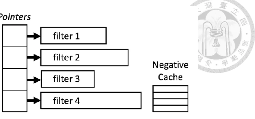
Figure 2 shows the high level architecture of ACF. It includes mainly 3 components – 1. Pointers of cuckoo filters (May be null pointer if no filter) 2. Cuckoo filters with variable size of buckets and fingerprint 3. A small hash table as negative cache.

The pointers each points to an instance of cuckoo filter and it may be null if its corresponding filter is not instantiated yet or is deleted to meet the overall memory budget. The amount of pointers is fixed and determined according to the max items that will be inserted.

Each filter is a cuckoo filter with variable number of buckets and size of fingerprint depending on the access frequency and false positive rate of the filter. A filter will grow to have more buckets or fingerprint size to lower its false positive rate because it has more access and generates more false positives before. In contrast, a filter will be shrunk to have less buckets or fingerprint size to sacrifice some of its occupied memory to the more accessed filters to meet the overall memory budget set initially. The additional negative cache is a small hash table storing true negative items in full repre- sentation to avoid frequent same false positive queries.

Figure 2. Architecture of ACF

Using an ACF, a point query (key) is processed as follows: First, a 128-bit hash value is gener- ated using the key - The first 32 bits are for indexing the pointer of filter, the second 32 bits are for indexing the bucket of the cuckoo filter and the third 32 bits are used as the key’s fingerprint (com- pressed representation). If the fingerprint is not found in one of its corresponding 2 buckets, the fil- ter returns false, indicating the query key doesn’t exist in the disk. If the fingerprint is found in one of the 2 buckets and the bucket’s false positive bit (indicating if the bucket has false positive before) is set to true, then check if the key is in the negative cache. If the key is in the negative cache, the filter returns false, otherwise returns true, indicating the key may be in the disk with high probabil- ity.

The data distribution is assumed as uniform since we use hash table to store data. How to make good use of space budget and adapt to skewed query distribution to achieve the lowest false positive rate is described in Chapter 4.4.

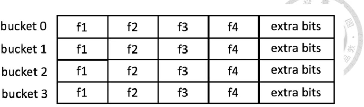
Figure 3. Data Structure of the Modified Cuckoo Filter

4.2 Data Structure

As suggested in [6], we choose (2, 4)-cuckoo filter (i.e., each item has two candidate buckets and each bucket have up to four fingerprints) that achieves the best or close-to-best space efficiency for the false positive rates that most practical applications may be interested. The configuration of the bucket size b = 4 has load factor α = 95% which is high enough in practical applications. Since cuckoo filters with semi-sorting are more space efficient than Bloom filters when 𝜖 < 3% and the minimal fingerprint size required is approximately:

𝑓 ≥ ⌈𝑙𝑜𝑔

(2𝑏/𝜖)⌉ = ⌈𝑙𝑜𝑔

(1/𝜖) + 𝑙𝑜𝑔

(2𝑏)⌉ (3)

and considering feasibility and efficiency of implementation, we choose the fingerprint size f to be 8, 12, 16, 20, 24, 28, 32 bits.

The original cuckoo filter utilizes a technique called partial-key cuckoo hashing to derive an item’s alternate location based on its fingerprint which is as follows (let nb be the number of buckets of a cuckoo filter):

ℎ

(𝑥) = hash(x) mod 𝑛𝑏, (4)

ℎ

(𝑥) = (ℎ

(𝑥) ⨁ hash(x

s fingerprint)) mod 𝑛𝑏

The exclusive or operation in Eq. (4) is an involution, ensuring a good property: To move a key originally in bucket i, we can calculate its alternative bucket j no matter i is ℎ₁(𝑥) 𝑜𝑟 ℎ₂(𝑥) by

𝑗 = (𝑖 ⨁ hash(fingerprint)) mod 𝑛𝑏. (5)

However, the xor operation will make the number of buckets of a filter only can be power of two which is not suitable for our design because we want to adjust each filter’s size in the fine-grained fashion.

To be able to have arbitrary number of buckets in a cuckoo filter, we use modular addition in place of exclusive or. But because modular addition is not an involution, we need to use an extra bit to remember if a fingerprint is in ℎ₁(𝑥) 𝑜𝑟 ℎ₂(𝑥). The revised partial-key cuckoo hashing is as fol- lows (let eb be the extra bit):

𝑗 = { (𝑖 + hash(x

s fingerprint)) mod 𝑛𝑏, 𝑖𝑓 𝑒𝑏 = 0

(𝑖 + 𝑛𝑏 − (hash(x

s fingerprint) % nb)) % 𝑛𝑏, 𝑖𝑓 𝑒𝑏 = 1 (6)

The additional space cost by the 4 extra bits in a bucket for the 4 fingerprint can be offset by using semi-sorting buckets optimization used in [6] to save one bit for each fingerprint. For the ease of implementation, we compact the 4 extra bits and one more bit that will be described in Chapter 4.5. The data structure is illustrated in Figure 3.

4.3 Operations

The operations that ACF can perform are same as cuckoo filter – Insert, Lookup and Delete.

Because ACF adopts an additional small negative cache, the algorithms of Insert and Lookup are different from the original cuckoo filter. Chapter 4.3.1 and 4.3.2 describes the algorithms of Insert and Lookup respectively.

4.3.1 Insert

Before inserting or looking up an item in ACF, we need to decide which filter to access, and after knowing which filter to access, the operation is mostly the same as cuckoo filter. Along with the all steps, we need to do 3 hashing – 1. Index the filter 2. Index the first bucket in the filter 3. Generate the fingerprint of the item. To optimize the hashing time, instead of calling 3 hash functions, we call only one hash function to get a 128-bit hash value including the three 32-bit hash value we need.

Because cuckoo filters have a load threshold. After reaching the maximum feasible load factor, insertions are non-trivially and increasingly likely to fail, so the hash table must expand in order to store more items. As shown in Algorithm 1. If an insertion failure occurs (line 7), we have to expand the filter. We need to read all the items originally in the filter from disk and re-insert them into the filter, also the item that caused failure. Besides, this newly inserted item may have caused false pos- itive and been inserted into the negative cache, so we need to clear the item in the negative cache if it’s there (line 12).

4.3.2 Lookup

The lookup process is shown in Algorithm 2. Given an item x, after indexing the filter to lookup, the algorithm does the normal lookup as cuckoo filter. The difference is – if the item is found in the filter and the bucket containing the item has false positive before (extra bit 𝑏₅ set to 1), it needs to check if the item is in the negative cache to avoid multiple duplicate false positives.

The philosophy of checking the negative cache after checking the filter is based on the idea of Victim Cache. Since the practical false positive rate is low (< 3%), only a small fraction of buckets

has false positives before. Thus, instead of checking the negative cache on every lookup, we only need to check the negative cache if the item’s fingerprint is found in the filter and the bucket contain- ing the fingerprint has false positives before. In this manner, we can save a lot of unnecessary negative cache lookups and make the lookup performance of ACF close to the original cuckoo filter.

4.4 Adaptive Strategy

ACF consists of multiple cuckoo filters, and each cuckoo filter may have different number of buckets and size of fingerprint to best fit the query distribution. Although we assume the data distri- bution is uniform in this thesis because of the usage of hash table, the structure of ACF can still adapt to data distribution.

This chapter shows the algorithms that can adjust the size of a cuckoo filter when needed. The concept is illustrated using an example - As in Figure 2, suppose at beginning, all the 4 filters are the same size as filter 1. As the lookup queries come, filter 2 and filter 4 grow bigger because the differences between their true false positive rate and target (theoretical) false positive rate are over a threshold. And filter 3 is shrunk smaller because the overall used memory is higher than the

memory budget and its lookup frequency is the smallest.

Unlike split Bloom filters [12] which use theoretical formulas to derive the size of each bloom filter to maintain the overall false positive rate, we use a heuristic strategy to change the size of cuckoo filters when needed as soon as possible. Because the origin of the skew comes from repeti- tive queries, but the optimal size calculated in SBF should be best for non-repetitive queries, it is more intuitive to use a heuristic approach to adapt to the skew as fast as possible.

4.4.1 Grow

Algorithm 3 gives the pseudo-code of the growing process. When a query q is processed and if it incurs false positive. It is checked whether the true false positive rate of the querying filter is higher than fp_threshold times of its target false positive rate. Also the amount of negatives of a fil- ter should be over a neg_threshold to achieve a certain statistic meaning. We will discuss how to choose these two thresholds in experiment 4. If the two conditions above are true, the filter should be grown. First, we need to determine whether to grow the size of buckets or the size of fingerprint.

We will only grow the size of fingerprint when the size of the filter’s empty buckets is over the ex- tra bytes if we grow the size of fingerprint. The reason is that we want to adjust the filter’ size in a

fine-grained way, and growing the fingerprint will make the filter grow “too much”, so we will grow the fingerprint if necessary. Besides, growing the fingerprint is better than growing the size of buckets to achieve lower false positive rate as (2) shows. Otherwise, we will only add 1 more buck- ets to the filter and maintain the same size of fingerprint. And since the filter only saves the finger- prints, we need to get the original keys from disk and re-insert them to the grown filter which will incur one disk access.

4.4.2 Shrink

Our goal is to minimize the false positive rate with a given memory budget. After a filter is grown, the overall used memory will increase and the overall false positive rate will decrease. How- ever, the size of the ACF may grow beyond its memory budget, so we need to shrink the ACF to fit the memory budget. Shrinking is done by choosing a victim filter and decrease its size of buckets or size of fingerprint. If the used memory is still beyond the budget, the shrinking process will be run iteratively until the used memory fits the budget.

To do shrinking, we have to find a victim filter to shrink carefully, because shrinking will in- crease the overall false positive rate. And we should choose the one that will have minimum effect of increasing the overall false positive rate. The strategy is straightforward – Find the least lookup filter, because it will incur least false positives compared to others. However, as the Algorithm 4 shows, we will shrink the filter’s fingerprint only if the filter’s buckets cannot be shrunk. To prevent shrinking fingerprint too often which will degrade the precision dramatically, we will consider the filters whose load factors are under a certain threshold as victims first, and then consider the filters with higher load factor.

4.5 Negative Cache

The negative cache is a small hash table storing the true negative keys in full representation.

The bigger the hash table is, the more negative keys can be saved which will avoid duplicate false positive queries and hence decrease the overall false positive rate. The tradeoff between the size of the negative cache and the predefined memory budget is not discussed in this thesis. This thesis only shows the effectiveness of decreasing the false positive rate in the skewed workload using only a small negative cache.

We adopt the second-chance strategy as the timing to insert a new false positive key into the negative cache. When a query key is a false positive query, we will not insert the key into the nega- tive cache immediately. Instead, we will insert a false positive key into the negative cache when the queried bucket has false positive queries before. Because the skewed workload will make some buckets have more false positives than other buckets, the second-chance strategy will prevent us from replacing the more-queried false positive keys with the less-queried false positive keys too of- ten.

As described in Chapter 4.3.2, the negative cache is treated as a victim cache, which will be queried only needed compared to a regular cache that is placed in the topmost position and need to be queried on every lookup. In this manner, we do not have to query the negative cache on every lookup, thus speeding up the lookup process. We need to query the negative cache only when the queried bucket in a filter has false positive queries before.

As described above, we need to know if a bucket of a filter has confronted false positive que- ries before. Therefore, we use one bit for each bucket save this information. We compact this one bit with the other 4 bits described in Chapter 4.2 in the extra bits as in Figure 3.

Chapter 5

Experiments

This chapter presents the results of the experiments that we conducted with the implementation of ACF, a synthetic benchmark and a real workload from BUSC server. We compare our method with 3 other methods – Cuckoo filter, Bloom filter and Split Bloom filters to study the false positive rate and the performance under the changing workload pattern. And we show the difference of lookup performance between ACF and Cuckoo filter. Specifically, this chapter shows the results of the fol- lowing two ACF variants:

 ACF: The complete design presented in Chapter 4.

 ACF no-NC: The ACF without the small negative cache (NC) and other components remains the same.

5.1 Benchmark Environment

To study ACF, we ran a series of synthetic workloads using the two ACF variants and other three types of filters – Cuckoo filter (CF), Bloom filter (BF) and split Bloom filters (SBF).

The benchmark database is uniformly distributed, which means the keys were evenly distributed in the domain, because ACF uses hashing to decide a key’s location, which will lead to uniform distribution naturally. The domain size of the inserted keys and queried keys is 2²⁴.

For experiment 1 and 2, we studied two different query workloads – Zipf and Uniform. All que- ries were generated randomly within the domain and run sequentially. For Zipf distribution, we study 9 different degree of skew. We vary the distribution parameter a of Zipf from 1.1 to 1.9. The bigger the a is, the more skewed the distribution is. The more skewed the workload is, the higher frequency the most-queried key has. We also studied a real workload from BUSC server that is also skewed.

For experiment 3 to 6, we use YCSB’s Zipf distribution with default parameters. Each data point in the figures is the average value of running 10 independent workloads.

All the experiments were conducted in the same way. First, we insert 200,000 distinct keys into ACF, CF, BF and SBF at the beginning. Then we ran 1,000,000 randomly generated queries accord- ing to the distributions stated before to measure the false positive rate. For lookup speed, we compare ACF to CF only. The false-positive rate is defined as the number of false positives divided by the total number of queried not in the filter. To be able to compare these 4 types of filters fairly, we make these filters use same amount of memory. To be specific, first, we insert the 200,000 keys into the ACF, and record its used memory which is set as the memory budget for all the 4 types of filters. For Cuckoo filter and Bloom filter, once the memory budget is set, the filter’s size is fixed. For ACF, occasionally the used memory will be a little bit higher than the memory budget but it will be shrunk to be below the budget through our shrinking algorithm. And for SBF, the used memory is dynamic and always below the budget.

5.2 Software/Hardware Settings

We ran all of the experiments on a machine with a 6-core Intel processor (3.40GHz) and 64GB of main memory. And the machine ran CentOS version 6.7. We implemented ACF based on the original C++ implementation by the author of Cuckoo filter. For Bloom filter, we use a Python pack- age, pybloom and revise it to be able to use a specified amount of memory. And we implemented split Bloom filters based on pybloom using Python. The split Bloom filters compared here is based on the design in [12] that all the Bloom filters will be resized to be their theoretical optimal size on every 10,000 lookups. We measured the execution time of ACF and Cuckoo filter using gettimeofday() function.

5.3 Experiment 1: False Positives

5.3.1 Synthetic Workload

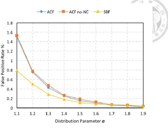
Figure 4a and 4b study the false positive rate of the two ACF variants and 3 other types of filters in the Zipf distribution with different distribution parameters. We show two different bits per item – 8 bit and 12 bit. The main competitor of ACF is split Bloom

Filters. Each point in the figures is the average of 10 independent experiments.

In Figure 4a and 4b, it’s clear that ACF and SBF can adapt to skewed workloads gracefully because they are designed to do so, so the more skewed the workload is, the better the precision is.

In Figure 4a, it can be seen that SBF has the smallest false positive rate in all different degree of skew. But it’s reasonable that our approach is not the best, because according to (1), (2), Cuckoo filter can only outperform Bloom filter in false positive rate when the bits per item is over 10 bits. Thus, in Figure 4b, when the bits per item is 12 bit, we can see that ACF is the clear winner in all degree of skew. Furthermore, the “ACF no-NC” variant is always worse than ACF, showing that we can have further improvement using only a small negative cache and proving the effectiveness of the negative cache described in Chapter 4.5.

Figure 6 shows the results under uniform workloads when the bits per item is 12 bit. It can be seen that ACF has higher false positive rate than Cuckoo filter, because it has no “skew” to adapt.

However, we can easily make ACF not adaptive by turning off the “grow” and “shrink” operation and not using negative cache to achieve the same precision as Cuckoo filter.

(a) Average bits per item = 8

(b) Average bits per item = 12

Figure 4. Zipf Workload, Vary Distribution Parameter

5.3.2 Real Workload

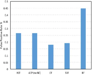
Figure 5 shows the results of experiment with the real workload from the Safe Box server which uses BUSC as its database engine. This workload is a query log during a short period of time, con- sisting of 200,000 insertions and 8,000,000 lookups from multiple users. The workload is also skewed because some objects are requested more often than other objects. In Figure 5, we can see that ACF outperforms other types of filters again. Besides, by using a small negative cache, the precision is improved phenomenally (halved from 0.06% to 0.03%).

.

Figure 5. BUSC Workload Figure 6. Uniform Workload

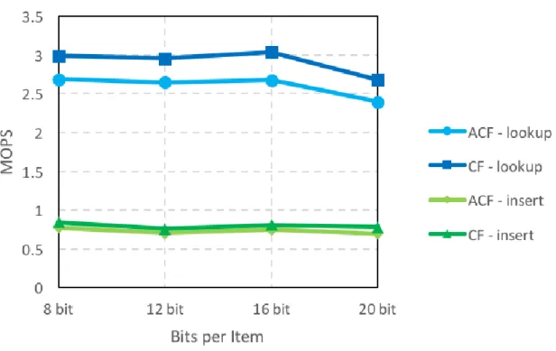
5.4 Experiment 2: Speed

In Figure 7, we can see that for lookup speed and insertion speed, ACF has a little bit perfor- mance degradation (7.4%~10.5%) than cuckoo filter. Because ACF has an added complexity of in- dexing the queried cuckoo filter, the use of extra bits and the use of negative cache, the query speed of ACF will be slower than cuckoo filter. However, this performance penalty is worth it, because we can save many unnecessary disk accesses that will lower the overall read throughput intensely.

In Figure 5, we can see that ACF has 4x lower false positive rate than cuckoo filter.

Figure 7. Lookup/Insert Speed

5.5 Experiment 3: Grow/Shrink Buckets

In this experiment, our goal is to determine how many buckets to grow/shrink at each time.

Figure 8 shows the results of growing/shrinking different number of buckets with limited/unlimited memory budget. With limited memory budget, the memory budget is set to the amount of used memory after inserting all keys into the ACF. In Figure 8a, it can be seen that as the number of growing/shrinking buckets increases, the shrinking times also increases steadily because it gets

more easily to exceed the tight memory budget. The more ACF shrinks, the higher false positive rate ACF has. We can observe that when growing/shrinking over 13 buckets at each time, the false positive rate will be higher than not growing/shrining at all (red line). In Figure 8b, we set the memory budget of ACF to be infinite, thus ACF will only grow but not shrink. It can be seen that the false positive rate does not decrease as we grow more buckets.

Therefore, we can view the process of growing more buckets of a filter as rehashing – just to

prevent the same false positive key from happening again. However, it is still possible that a filter will confront multiple different false positive keys. But, since ACF uses many filters, it has a small probability that multiple high-frequency keys will locate in the same filter. Even if this situation happens, ACF can adapt to it quickly.

In conclusion, we choose to grow/shrink 1 bucket at each time. In other words, we adjust ACF in the most fine-grained way, and this will lead to the best performance.

(a) Limited Memory Budget

(b) Unlimited Memory Budget

Figure 8. Limited/Unlimited Memory Budget, Vary Grow/Shrink Buckets

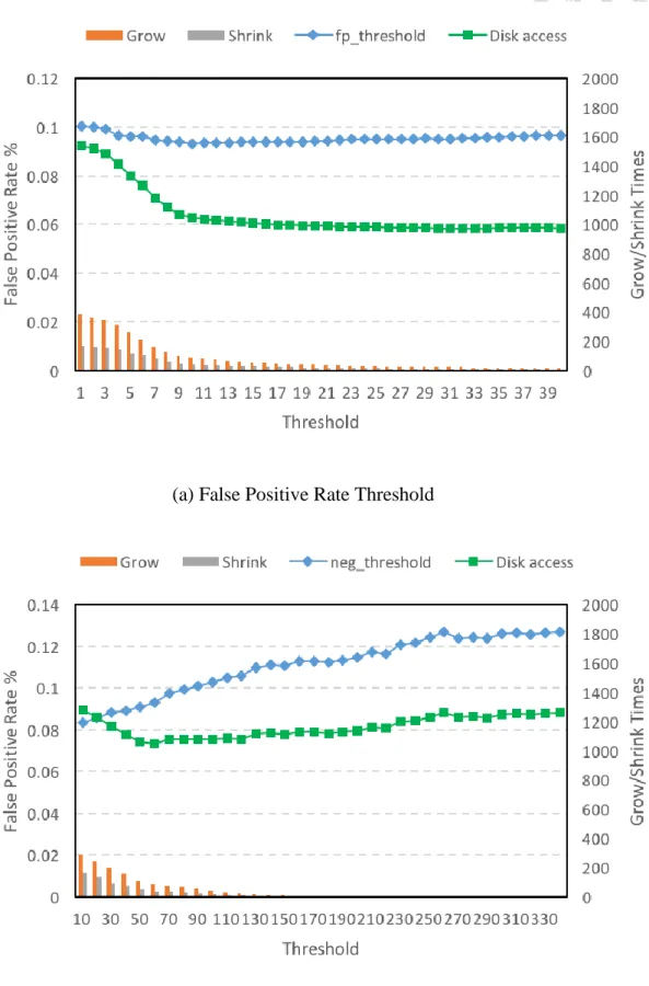
5.6 Experiment 4: Grow Threshold

In this experiment, we aim to choose the appropriate threshold value of fp_threshold and neg_threshold in Algorithm 3. The bigger the threshold value is, the less frequent will ACF grow.

We do not want to grow too much because every growing will cause a disk access, and it might in- cur more shrinking which will also cause disk accesses. In contrast, if we grow too conservatively, we cannot adapt to the skewed pattern properly. Thus, we need to choose a good balance between the two extremes.

Figure 9 shows the results of the tuning of the two threshold values. We show two lines – false positive rate and total disk accesses. Disk access includes the total disk accesses caused by false positives and growing/shrining. In Figure 9a, we fix neg_threshold to 60 and vary fp_threshold from 1 to 40. We can observe that when fp_threshold = 10, the false positive rate is at the mini- mum, and the total disk access stop decreasing. Thus, we choose 10 as the value of fp_threshold.

In Figure 9b, we fix fp_threshold to 10 and vary neg_threshold from 10 to 340. Although the false positive rate increases linearly as fp_threshold increases, the total disk accesses is at the minimum when neg_threshold = 60. Thus, we choose 60 to be neg_threshold.

The reasoning behind choosing the right threshold is that we want ACF to react in the best tim- ing while maintaining the false positive rate low but not causing too much growing/shrink which will offset the benefit of low false positive rate.

(a) False Positive Rate Threshold

(b) Negative Threshold

Figure 9. Vary Thresholds (fp_threshold, neg_threshold) in Algorithm 3

5.7 Experiment 5: Negative Cache

In this experiment, we aim to choose the proper size of the negative cache and show the ad- vantages of adopting second-chance strategy and treating the negative cache as a victim cache. We turn off the functionalities of growing/shrinking, thus ACF only uses the negative cache to adapt to skewed workload in this experiment.

5.7.1 Negative Cache Size

In Figure 10a, we can observe that the false positive rate decreases as the size of the negative cache increases, which is intuitive because the negative cache can store more false positive keys and the keys stored in the negative cache are less likely to be replaced by others.

We can observe that there is a turning point when the negative cache has 12 buckets, and after- ward the false positive rate decreases slowly. Because only a small fraction of the keys are frequently accessed, we can capture the skewness using a small size of negative cache. After the turning point, it will be less effective of adding more buckets to the negative cache. Moreover, since the keys in the negative cache is in its complete representation, not compressed, we should make the negative cache as small as possible. Therefore, we choose 12 buckets, the turning point, as the negative cache heu- ristically.

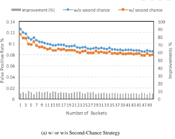
5.7.2 Second-Chance Strategy and Victim Cache

In Figure 10a, it can be seen that adopting second-chance strategy achieves consistently lower false positive rate than not adopting, leading to the average 8% improvements.

In Figure 10b, we place the negative cache before ACF (as regular cache) or after ACF (as victim cache) to find which one has better lookup performance. We can observe that the size of the negative cache will not affect the lookup performance, and treating the negative cache as a victim cache achieves consistently better performance, resulting in the average 15.4% improvements.

(a) w/ or w/o Second-Chance Strategy

(b) Victim Cache

Figure 10. Effect of Second-Chance Strategy and Victim Cache

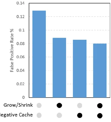
5.8 Experiment 6: Combinations

Figure 11 shows the different combinations of ACF adopting Grow/Shrink strategy or Nega- tive Cache or both. We can see that adopting Grow/Shrink strategy solely can achieve 31.4% im-

provements compared to the not adaptive version (the first bar). Using negative cache solely can achieve 33.5% improvements. If we combine both the two adaptive strategies, then we can achieve 38% improvements, getting additional 7% and 5 % improvements than using only one of the two adaptive strategies.

Figure 11. Combinations

Chapter 6

Conclusion

This thesis presented ACF, a new data structure called Adaptive Cuckoo Filters (ACF). ACF can exploit the skewed access pattern and dynamically adjust the size of an array of cuckoo filters to achieve significant smaller false positive rate than a single cuckoo filter. In addition, ACF uses a small hash table as Negative Cache which stores false positive keys to further lower the false positive rate. We determined the best parameters for ACF and proved the effectiveness of adopting second- chance strategy and treating the negative cache as a victim cache through experiments. Extensive experiments showed that when the workload is skewed, ACF can outperform traditional Bloom filters and cuckoo filters, and a state-of-the-art split Bloom filters that can also adapt to skewed workload.

For future work, we plan to do the quantitative analysis of ACF and develop a mathematical framework for optimizing ACF under various query distributions.

Bibliography

[1] A. Rousskov and D. Wessels. 1998. Cache digests. In Computer Netw. ISDN Syst., vol. 30, no.

22–23, pp. 2155–2168.

[2] A. Malik and P. Lakshman. 2010. Cassandra: a decentralized structured storage system. In SI- GOPS Operating System Review, vol. 44, no. 2.

[3] A. Eldawy, J. J. Levandoski, and P. Larson. 2014. Trekking through Siberia: Managing cold data in a memory-optimized database. In Proc. Int. Conf. Very Large Data Bases, pp. 931–942.

[4] B. H. Bloom. 1970. Space/time trade-offs in hash coding with allowable errors. Communica- tions of the ACM, 13(7):422–426.

[5] Bruck, J., Gao, J., and Jiang, A. 2006. Weighted Bloom Filter. In IEEE International Sympo- sium on Information Theory.

[6] Bin Fan, Dave G. Andersen, Michael Kaminsky, and Michael D. Mitzenmacher. 2014. Cuckoo filter: Practically better than Bloom. In Proc. 10th ACM Int. Conf. Emerging Networking Exper- iments and Technologies (CoNEXT ’14), pages 75–88, 2014. doi:10.1145/2674005. 2674994.

[7] C. Diaconu, C. Freedman, E. Ismert, P.-A. Larson, P. Mittal, R. Stonecipher, N. Verma, and M.

Zwilling. 2013. Hekaton: SQL Server’s memory-optimized OLTP engine. In SIGMOD, pages 1–12.

[8] D. N. Simha, M. Lu, and T.-c. Chiueh. 2012. An update aware storage system for low-locality update intensive workloads. In Proceedings of the International conference on Architectural Support for Programming Languages and Operating Systems, pages 375–386. ACM.

[9] F. Putze, P. Sanders, and S. Johannes. 2007. Cache-, hash- and space efficient bloom filters. In Experimental Algorithms, pages 108–121. Springer Berlin / Heidelberg.

[10] J. K. Mullin. 1990. Optimal semijoins for distributed database systems. In IEEE Trans. Soft- ware Eng., 16(5):558–560.

[11] L. Fan, P. Cao, J. Almeida, and A. Z. Broder. 1998. Summary cache: A scalable wide-area Web cache sharing protocol. In Proc. ACM SIGCOMM, Vancouver, BC, Canada.

[12] L. Sidirourgos and P.Å . Larson, Adjustable and Updatable Bloom Filters. Available from the authors.

[13] N.P.Jouppi. 1990. Improving direct-mapped cache performance by the addition of a small fully-associative cache and prefetch buffers. In 17th Annual International Symposium on Com- puter Architecture. doi:10.1109/ISCA.1990.134547

[14] Zhong, M., Lu, P., Shen, K., and Seiferas, J. 2008. Optimizing Data Popularity Conscious Bloom Filters. In Proceedings of the 27th ACM symposium on Principles of Distributed Compu- ting.