基於後向切割的等效驗證和工程變更指令演算法之最佳化

(1)

國立臺灣大學電機資訊學院電機工程學研究所碩士論文

Graduate Institute of Electrical Engineering

College of Electrical Engineering and Computer Science

National Taiwan University Master Thesis

基於後向切割的等效驗證和工程變更指令演算法之最佳化 Optimizing Backward-Cut-Based EC and ECO Algorithms

李友岐 Yo-Chi Lee

指導教授：黃鐘揚博士

Advisor: Chung-Yang (Ric) Huang, Ph.D.

中華民國 108 年 7 月

July, 2019

(2)

摘要

在晶片設計的流程中，如果流程後期需要修改原本的電路設計，工程變更指令是一個普遍使用的方法。我們提出新的演算法以優化基於後向切割的工程變更指令引擎效能。我們藉著後向切割在兩個電路中找出改正配對，接著精鍊這些配對以去除多餘的部份。實驗結果顯示我們提出的演算法不但減少了修補邏輯電路的成本也降低了程式運行的時間。除此之外，我們進一步將後向切割應用於等效驗證，實驗結果說明了我們的演算法是可行的。

關鍵詞：工程變更指令、後向切割、修補邏輯電路、等效驗證

(3)

ABSTRACT

Engineering change order (ECO) is a popular approach for rectifying circuit errors and specification changes in late design stages. Backward-cut-based ECO solves the problem by divide and conquer from the output side to input side. In this thesis, we present new algorithms to optimize the performance of ECO engine. We first discover the rectification pairs in two circuits by backward-cut approach and then remove the redundant parts by refinement technique. The experimental results show that our algorithm not only reduce the patch circuit cost but also improve the run time of ECO engine. Moreover, we further apply backward-cut approach to the Equivalence Checking (EC) and experimental results prove that our algorithms work.

Index Terms – Engineering change order, backward-cut, patch circuit, equivalence checking.

(4)

LIST OF FIGURES

Fig. 1 IC Design Flow and the purpose of a functional ECO tool. [4] ... 2

Fig. 2 A functional ECO example. [4] ... 2

Fig. 3 Resource-aware functional ECO. [5] ... 3

Fig. 4 Definition of backward and forward direction in a circuit ... 5

Fig. 5 A miter example. [10] ... 7

Fig. 6 And-inverter graph example ... 8

Fig. 7 Structural hashing example ... 8

Fig. 8 Functionally reduced and-inverter graph algorithm. [8]... 9

Fig. 9 Single-fix interpolation circuit. [17] ... 11

Fig. 10 Partial-fix interpolation circuit. [19] ... 11

Fig. 11 Cofactor reduction algorithm. [20] ... 12

Fig. 12 The main phases of DeltaSyn. [14]... 13

Fig. 13 Match-and-Replace ECO. [7]. ... 14

Fig. 14 Cut-matching algorithm in [7]. ... 15

Fig. 15 Matching matrix in [7] ... 15

Fig. 16 An example of rectification pairs. [7] ... 17

Fig. 17 Basic output-side frontier identification algorithm... 22

Fig. 18 Overview of our dual-phases ECO engine ... 23

Fig. 19 The backward-cut-based ECO. ... 24

Fig. 20 An example of using merged gates to construct patch. [8] ... 26

Fig. 21 Output-side identification algorithm... 27

Fig. 22 The simulation of cut pair candidate ... 28

Fig. 23 Cut-matching algorithm ... 29

(7)

Fig. 24 Rectification pair selector. [7]... 31

Fig. 25 Rectification pair refinement algorithm... 31

Fig. 26 The illustration of further cut-matching approach ... 34

Fig. 27 The repeatedly solving algorithm. ... 35

Fig. 28 Backward-cut-based EC algorithm ... 37

Fig. 29 The change of patch size after each iteration... 51

Fig. 30 The change of patch size in iteration #1 ... 51

Fig. 31 The change of patch distribution after each iteration ... 52

(8)

LIST OF TABLES

Table 1 Performance comparison under the testcases modified from [29]. ... 40

Table 2 Performance comparison under the testcases modified from [5] ... 41

Table 3 Performance comparison between solving repeatedly and one time ... 42

Table 4 Performance comparison between with and without Method #1 ... 44

Table 5 Performance comparison between with and without Method #2. ... 45

Table 6 Performance comparison between with and without Method #3 ... 46

Table 7 Performance comparison between forward and backward approach ... 48

(9)

Chapter 1 Introduction

In VLSI design flow, late design changes are inevitable and the complexity to handle these changes is increasing since the modern design size is growing rapidly. If these design changes occur towards the end of the design cycle, it is impractical to go through the entire VLSI design flow again due to the time-to-market pressure. Moreover, significant time and efforts already spent on the original design would be wasted. To deal with this problem, a method called Engineering Change Order (ECO) was proposed to keep these changes local [1]-[3]. Fig. 1 and Fig. 2 show the purpose and an example of ECO. RTL 1 is the original design while RTL 2 represents the new specification, which can be viewed as the golden design. Instead of generating a whole new converged netlist for the golden design, we compare the original converged netlist with the netlist synthesized from the golden RTL by ECO tool. In other words, we want to find the minimal difference between the original and the golden (new) circuits. The identified logic difference is called the patch, which can be implemented by technology mapping with spare cells. More specifically, spare cells are the extra cells inserted to the design for the ECO purpose. Normally, they have nothing to do with the function of original design. We can then realize the function of computed patch with the available spare cell resource. As a result, there is no need to restart the whole design flow from scratch. Since the original design is usually optimized after a series of processes, it is hard to revise the

(10)

netlist to bring in the corresponding RTL changes. Therefore, we need an ECO engine to automatically implement these changes.

Fig. 1. IC design flow and the purpose of a functional ECO tool. [4]

Fig. 2. A functional ECO example. [4]

(11)

ECOs can be divided into functional ECO and timing ECO. Functional ECO handles the logical changes to the design, while timing ECO concentrates on improving the performance of design or repairing timing violations caused by the specification changes. For functional ECO, the target is to fix the logic difference between the original and the golden circuits and to make the size of resulted patch as small as possible. By adding the patch to the original circuit, two circuits should become functionally equivalent. During this stage, we usually focus on the rectification of logic function. In contrast, when dealing with timing ECO, we need to consider the physical constraints, such as the location of spare cells and the wiring length of composing patch. Recently, some researches consider physical issues simultaneously when handling functional correction, which is called resource-aware functional ECO [5] [6]. Fig. 3 presents the concept of resource-aware functional ECO.

Fig. 3. Resource-aware functional ECO. [5]

(12)

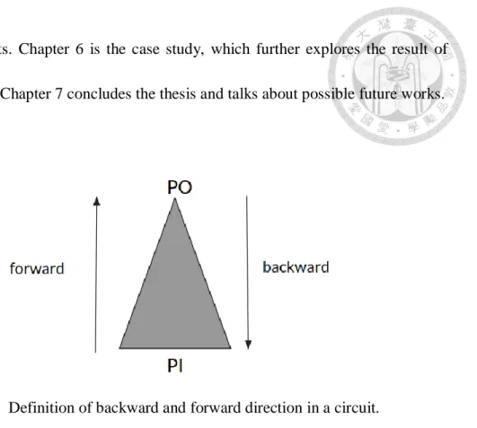
In this thesis, however, we only discuss the solution to pure functional ECO problems. That is to say, we consider no physical constraint during the process and focus on how to make the given two circuits functionally equivalent with minimal patch. We usually solve the ECO problem by divide and conquer since the modern designs are too large. Some researches narrow down the problem by iteratively finding equivalence cuts for the original and the golden circuits. We call this approach backward-cut since it generates cuts from the output side to the input side of circuits. Fig. 4 illustrates the definition of backward and forward direction in a circuit. Both of [7] and [8] demonstrate the backward-cut-based ECO techniques.

Past researches, however, still have room for improvement. As a consequence, we propose a two-phases approach, which optimizes backward-cut-based ECO algorithms in [7] and [8]. Our approach contains two phases: 1) merging phase: to find the gates in the original and golden circuits which are functionally equivalent to each other and then merge them into one gate; 2) matching phase: to explore the matches between the original and golden circuits in order to identify the minimal regions for rectification. In addition, we further apply this backward-cut approach to equivalence checking, which is usually solved forwardly. Experimental results show that our idea works.

The remainder of this paper is organized as follows. Chapter 2 gives some preliminaries. Chapter 3 describes our backward-cut-based ECO algorithm in detail.

Chapter 4 shows our backward-cut-based EC algorithm. Chapter 5 discusses our

(13)

experimental results. Chapter 6 is the case study, which further explores the result of particular testcase. Chapter 7 concludes the thesis and talks about possible future works.

Fig. 4. Definition of backward and forward direction in a circuit.

(14)

Chapter 2 Preliminaries

In this chapter, we present the prior knowledges related to our work. First, chapter 2.1 ~ 2.4 describe the fundamental concepts we need for ECO. Chapter 2.5 and 2.6 briefly introduces previous works and the criteria of ECO problem, respectively. The techniques proposed in past researches are then described in the remaining chapter.

2.1 Boolean Satisfiability

Boolean satisfiability problem (SAT) is a decision problem taking a propositional formula which represents a Boolean function. It would answer whether this formula is satisfiable. The formula is satisfiable (SAT) if there is at least an input assignment to evaluate the formula to 1 (true). Otherwise, the propositional formula is unsatisfiable (UNSAT). If the formula is unsatisfiable, then the Boolean function is proved to be a constant 0. A SAT solver is a software program for solving SAT problems. When a SAT problem is satisfiable, the solver returns SAT with a satisfying assignment. Our ECO engine adopts Minisat [9], which is the most popular SAT solver over the world.

2.2 Equivalence Checking (EC) & Miter

Two circuits are regarded as functionally equivalent if and only if their output values are equal under all input assignments. Equivalence checking plays an important role in functional ECO. In the ECO process, we need to check the functional

(15)

correctness after circuit rectification. If two circuits are non-equivalent, it means that there are still errors in the circuit. We usually transform the equivalence checking problem to a satisfiability problem with a miter [10]. If we want to check the functional equivalence between two Boolean networks F (Original) and G (Golden), then we build a miter like Fig. 5, which applies an exclusive-or gate (XOR) to F and G. They are functionally equivalent if and only if there is no input assignment making the miter outputs 1. That is, two Boolean networks F and G are functionally equivalent if and only if the miter of F and G is UNSAT.

Fig. 5. A miter example in [10].

2.3 AIG, Strash & FRAIG

And-inverter graph (AIG) is a directed and acyclic graph that represents a structural implementation of the logic circuit. In AIG structure, each node represents an AND gate and contains two inputs. Each input includes a node it connects to and a flag

(16)

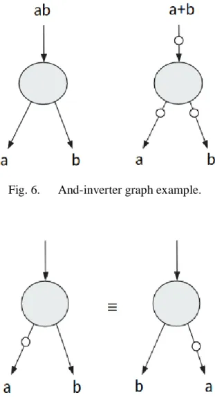
to signify whether this input is inverted. Since {AND, NOT} is a functionally complete set, every Boolean function can be transformed into an AIG. Fig. 6 illustrates two simple AIG examples. Normally, when a circuit problem is modeled in AIG, the implementation can be simplified due to the simplicity of the AIG data structure and thus the room to optimize the algorithm will become larger. For example, to speed up equivalence checking, AIG-based Strash and FRAIG are two commonly used techniques. We can also utilize the merged gates discovered in these two processes to guide the pairing during cut- matching.

Fig. 6. And-inverter graph example.

Fig. 7. Structural hashing example.

(17)

Structural hashing (Strash) is to map each AND gate and its two inputs into a canonical form. Fig. 7 shows the concept of structural hashing. With this method, we can efficiently discover some equivalent gates and then merge them.

Functionally reduced and-inverter graph (FRAIG) [11] technique first find the functional equivalent candidates (FEC) by simulation and then check whether they are actually equivalent by SAT solver. The algorithm is presented in Fig. 8.

Algorithm Functionally-Reduced And-Inverter Graph 1: Input: Circuit ckt

2: Output: Circuit ckt

3: solver ⟵ Init_Proof_Model(ckt)

4: classes ⟵ Init_FEC_By_Random_Simulation(ckt) 5: for each gate g in ckt in a topological order do 6: fec ⟵ Get_FEC(classes, g)

7: if fec == null then continue 8: for each m in fec do

9: if Sat_Check_Equivalence(solver, g, m) == UNSAT then 10: Merge(ckt, g, m)

11: else

12: pattern ⟵ Get_Sat_Pattern(solver)

13: classes ⟵ Simulate_And_Update_FEC(classes, pattern) 14: end for

15: end for Fig. 8. Functionally reduced and-inverter graph algorithm. [8]

2.4 Boolean Matching

Boolean matching is a problem determining the functional equivalence between two Boolean functions under permutations and negations of their inputs and outputs. In logic synthesis and verification, Boolean matching has been widely adopted.

(18)

Besides, it has also been applied to the backward-cut matching in the functional ECO and the technology mapping. Given two Boolean functions f(X¹) and g(X²) with same amount of inputs (|X¹| = |X²|). Boolean matching under NPN-equivalence decides whether f and g can be functionally equivalent or complementary under negations and permutations of the variables of X¹ and X². The first and second “N” in “NPN” represent the negations on the inputs and outputs, respectively. The “P” means the permutations on the inputs. In our ECO technique, we apply a simulation-guided cut-matching algorithm to discover the output-side boundaries of the patch, which can be viewed as an NP-equivalent Boolean matching problem. We check the equivalence between two circuits under the negations and permutations on the inputs but the negations on the outputs are excluded. Moreover, the boundaries are not predefined in our cut-matching process so we need to search for the matching candidates first.

2.5 Previous Works on Functional ECO

There are many works focusing on functional ECO in recent years. [12]–[14]

propose fault models to describe the design errors, such as incorrect gate-type, inverter missing, and wire misplaced. These techniques rectify the buggy designs based on their fault models. As a result, the patch circuits are usually predictable. In most cases, however, these techniques fail to generate the patch circuit since the fault models are not enough to represent the functional difference.

(19)

Fig. 9. Single-fix interpolation circuit in [17].

Fig. 10. Partial-fix interpolation circuit in [19].

Synthesis-based ECO algorithms [15]–[19] explore an internal rectification signal by some diagnosis approaches, and then produce a patch function for the functional difference by re-synthesis techniques. Despite the fact that these algorithms are able to automate the functional ECO flow, relying on a single-fix signal is their main disadvantage, as Fig. 9 shows. In the worst case, the only possible single-fix signal is the primary output itself in real-world testcases. Therefore, the resulted patches may be

(20)

extremely large, which is unacceptable. In order to handle these problems, a partial-fix interpolation-based ECO engine is proposed in [19]. This ECO engine generates partial rectifications iteratively and thus incrementally fix multiple errors in the design as Fig.

10 shows. Although this technique can deal with the problem more efficiently, it considers the errors in the design to be independent. However, there may be some correlations between the errors in circuit. As a consequence, the iterative process may not be able to converge. A cofactor reduction algorithm in [20] is applied to generate multi- fix rectification patches by interpolation, which takes multiple errors into consideration simultaneously. Fig. 11 presents the algorithm in [20].

Fig. 11. Cofactor reduction algorithm in [20].

(21)

Sweeping-based ECO algorithms are proposed in [21]–[24]. They demonstrate a structural comparison between the original and golden circuits. Due to the fact that the functional rectifications in RTL often comes from small and local changes, sweeping- based approaches are very rational for functional ECO. DeltaSyn [24] proposes a dual- phase flow to first identify the input-side and output-side frontiers of the changes and then collect the logic gates within two frontiers to be the patch circuit, as Fig. 12 shows.

[25] and [26] provide efficient forward sweeping algorithms to merge the functionally equivalent gates and then derive the input-side boundary between the original and the golden circuits. Nevertheless, it still remains a huge challenge to discover the output-side matching boundary. The computational complexity of output-side matching algorithm is usually much higher.

Fig. 12. The main phases of DeltaSyn. [24]:

(a) The original and the modified specification (ECO) are given as inputs.

(b) Input-side boundary of the changes are identified.

(c) Output-side boundary of the changes are located and verified.

(22)

Match-and-Replace (M&R) [7] explores functional matches in the original and golden circuits by the cut matching algorithms and SAT-sweeping technique. Fig. 13 and Fig. 14 illustrate the concept of M&R and the flow of cut-matching algorithm. In the matching phase, M&R first discovers the matched gates (g, g’) of two circuits, where

gates g and g’ are in the original and the golden circuit, respectively. After that, M&R enumerates a cut from the matched gate g randomly, and then gradually selecting the candidate gates according to the selected cut of g and the matched gate g′. To get the matched cut, the SAT-based matching is applied by constructing a matching matrix shown in Fig. 15.

Fig. 13. Match-and-Replace ECO. [7]

(23)

Fig. 14. Cut-matching algorithm in [7].

Fig. 15. Matching matrix in [7].

(24)

Since M&R generates the cut from the matched gate g without a clue, the matching process is extremely time-consuming. Besides, even though we find a matched cut, the quality of the matched cut pairing might be poor, which would lead to large patch size. As a result, [8] proposes a semi-formal ECO method, where the simulation-guided cut-matching algorithm is applied to render a clue based on circuit similarity in matching the cuts. Since ECO usually means that multiple design errors or specification changes occur in the original circuit and need to be rectified, the gates affected by the buggy gate might be functionally non-equivalent with the corresponding gates in the golden circuit.

The functional difference between these gates, however, is hard to be observed. In other words, the values of these gates are different in a few input patterns only and are the same for most of them. Therefore, the two gates might be a promising pairing if their responses are highly similar. In some multi-errors ECO testcases, however, the performance of [8]

is not as good as we expect, which implies that there is still room for improvement. Thus, we optimize the algorithms in [8] and propose a more efficient ECO engine.

2.6 ECO Problem Formulation and Optimization Criteria

Given two circuits: original and golden, which are functionally non-equivalent to each other. Our ECO engine takes original and golden as inputs and outputs the patched circuit. The patched circuit is rectified from original circuit and functionally equivalent to the golden circuit. The functional equivalence between the patched and golden circuit

(25)

is verified by the academic tool ABC [27] using cec command. All circuits are described in AIGER [28], which is a circuit format for AIG.

Accommodating RTL changes with little rectification to the original converged design is the core objective of a functional ECO. Therefore, the basic criterion for the ECO tool is to make the ECO changes (patch), called “patch size”, as small as possible.

The second important criterion is the run time of the ECO tool. Since ECOs are often done at the later stage of a project, which is very close to Tape Out, we only have limited time to handle it. The process of an ECO tool should be finished within a reasonable time.

2.7 Rectification Pair

Fig. 16. An example of rectification pairs. [7] (a) Cir1. (b) Cir2.

(e, f) and (g, c) are a pair of matched cuts from h ↔ i.

Thus, e ↔ g and f ↔ c are their rectification pairs.

The idea of rectification pair is first introduced by [7]. The definition is shown as follows according to [7]:

(26)

Definition 1: A set of pairs RP_Set: 𝑔 ⃗⃗⃗ ↔ 𝑔 ⃗⃗⃗ ′ is called a set of rectification pairs if each 𝑔_𝑖 ∈ 𝑔 ⃗⃗⃗ belongs to the original circuit and 𝑔′_𝑖 ∈ 𝑔 ⃗⃗⃗ ′ belongs to the golden one, and the original circuit becomes functionally equivalent to the golden one after replacing every 𝑔_𝑖 with 𝑔′_𝑖.

For a rectification pair (𝑔_𝑖, 𝑔′_𝑖), 𝑔_𝑖 is called the patched gate and 𝑔′_𝑖 is its corresponding patch. With the rectification pair, the rectification of functional equivalence can be formulated as

∀X, Ori (X)|

𝑔

⃗⃗⃗ ^Ｒ← 𝑔 ⃗⃗⃗ ^′(X) ≡ Gold (X) (1) where X is the primary inputs, and 𝑔 ⃗⃗⃗ ← 𝑔 ^Ｒ ⃗⃗⃗ ′(X) represents the operation of replacing each 𝑔_𝑖 ∈ 𝑔 ⃗⃗⃗ with 𝑔′_𝑖 ∈ 𝑔 ⃗⃗⃗ ′.

Please note that it is always possible to derive a set of rectification pairs to fix the functional differences between the original and the golden circuits. For instance, the primary output (PO) pairs form a trivial set of rectification pairs naturally. Thus, replacing all outputs in the original circuit with the outputs in the golden circuit is definitely a solution to rectification. The patch size, however, might be unacceptably large. The following lemma introduces an iterative approach to reduce the patch size:

Lemma 1: Given a rectification pair P: 𝑔_𝑖 ↔ 𝑔′_𝑖 ∈ RP_Set, 1 ≤ i ≤ n and a set of

pairs P_Set: ℎ ⃗⃗⃗ ↔ ℎ ⃗⃗⃗ ^′ , the set (RP_Set − {P} + P_Set ) is also a set of rectification pairs if P_Set is a set of rectification pairs of P.

Proof: Since

∀X, Ori (X)| Ｒ _′ ≡ Gold (X). (2)

(27)

If a set of pairs P_Set: ℎ ⃗⃗⃗ ↔ ℎ ⃗⃗⃗ ′ is a set of rectification pairs of pair P : 𝑔_𝑖 ↔ 𝑔′_𝑖, which can be formulated as

𝑔_𝑖(X)|

⃗⃗⃗ ℎ ^Ｒ← ℎ ⃗⃗⃗ ′(X) ≡ 𝑔′_𝑖(X) (3) by (2) and (3)

∀X, Ori (X)|

𝑔 ⃗⃗⃗ [1,i−1]^Ｒ← 𝑔 ⃗⃗⃗ ^′[1,i−1](X), 𝑔 ⃗⃗⃗ [i+1,n]^Ｒ← 𝑔 ⃗⃗⃗ ^′[i+1,n](X), ℎ ⃗⃗⃗ ^Ｒ← ℎ ⃗⃗⃗ ^′(X) ≡ Gold (X) (4) where 𝑔 ⃗⃗⃗ [1, i−1] denotes the concatenation of {𝑔₁, 𝑔₂,... , 𝑔_𝑖−1} and g [i+1, n] denotes the concatenation of {𝑔_𝑖+1, 𝑔_𝑖+2,... , 𝑔_𝑛}.

By (4), ( RP_Set − {P} + P_Set ) must also be a set of rectification pairs of Ori(X).

According to the above lemma, we can iteratively derive a set of new rectification pairs on the existing pairs. [7]

2.8 Cut Function

In our ECO engine, we discover new rectification pairs by a cut-matching algorithm, which finds two cut function in original circuit and golden circuit, respectively. After replacing the cut in original circuit with the other cut, the two circuits become functionally equivalent. According to [7], the cut function is defined as follows:

Definition 2: Given a cut (𝑔₁, 𝑔₂,... , 𝑔_𝑛) in circuit Cir, a cut function 𝐶𝐹_{𝐶𝑖𝑟 (𝑔}₁_,𝑔₂_,...,𝑔_𝑛₎ represents the function of the circuit with respect to (𝑔₁, 𝑔₂,... , 𝑔_𝑛).

As Cir1 in Fig. 16(a) shows, the output function with respect to (a, b, f ) is

(28)

h(a, b, c, f )=(a+b)f and the cut function of the cut (a, b, f ) is 𝐶𝐹_{ℎ(𝑎,𝑏,𝑓 )}(x1, x2, x3) = (x1 + x2)x3, where (x1, x2, x3) are the corresponding input variables of h on (a, b, f ). We say two cut functions are equivalent if

𝐶𝐹_{𝐶𝑖𝑟( 𝑔}_{⃗⃗⃗ )}(X) ≡ 𝐶𝐹_𝐶𝑖𝑟^′_{( 𝑔}_⃗⃗⃗^′₎(X)

is valid.

Given two equivalent cut functions, called matched cuts, the rectification pairs can be easily derived by the following theorem:

Theorem 1: Given two cuts 𝑔 ⃗⃗⃗ : (𝑔₁, 𝑔₂,... , 𝑔_𝑛) and 𝑔 ⃗⃗⃗ ^′: (𝑔′₁, 𝑔′₂, 𝑔′_𝑛 ) in circuits 𝐶𝑖𝑟 and 𝐶𝑖𝑟^′, respectively, if 𝐶𝐹_{𝐶𝑖𝑟( 𝑔}_{⃗⃗⃗ )}and 𝐶𝐹_𝐶𝑖𝑟^′_{( 𝑔}_⃗⃗⃗^′₎ are equivalent, then 𝑔 ⃗⃗⃗ ↔ 𝑔

⃗⃗⃗ ′ is a set of rectification pairs and the revised circuit 𝐶𝑖𝑟^′′(X) : 𝐶𝑖𝑟(X) |

𝑔

⃗⃗⃗ ^Ｒ← 𝑔 ⃗⃗⃗ ^′(X) will be functionally equivalent to C𝑖𝑟^′(X).

Proof: Since the cut functions 𝐶𝐹_{𝐶𝑖𝑟( 𝑔}_{⃗⃗⃗ )}(X) ≡ 𝐶𝐹_𝐶𝑖𝑟^′_{( 𝑔}_⃗⃗⃗^′₎(X), if 𝐶𝑖𝑟 and 𝐶𝑖𝑟^′ are not functionally equivalent, it must result from the functional differences between 𝑔 ⃗⃗⃗

and 𝑔 ⃗⃗⃗ ′. Once we do the replacement for every pair in ( 𝑔 ⃗⃗⃗ , 𝑔 ⃗⃗⃗ ^′ ), 𝑔 ⃗⃗⃗ become equivalent to 𝑔 ⃗⃗⃗ ^′. Thus, after replacing, the revised circuit 𝐶𝑖𝑟^′′(X) : 𝐶𝑖𝑟(X) |

𝑔

⃗⃗⃗ ^Ｒ← 𝑔 ⃗⃗⃗ ^′(X) will be functionally equivalent to C𝑖𝑟^′(X).

Concluding the above descriptions, we are able to derive the rectification pairs from the matched cuts. In addition, given a rectification pair where two gates are functionally non-equivalent, we can iteratively find a matched cut for this pair and thus identify more rectification pairs. Therefore, we will keep getting new rectification pairs with smaller patches after each iteration. [7]

(29)

2.9 Similarity between the Candidate Gates

Exploring equivalent cut function is an important part of cut-matching. However, the inputs of cut function, such as 𝑔 ⃗⃗⃗ and 𝑔 ⃗⃗⃗ ^′, are not yet defined. Therefore, we need to

find 𝑔 ⃗⃗⃗ and 𝑔 ⃗⃗⃗ ^′ before checking the equvalence of two cut functions. [8] proposed a simulation-guided cut-matching approach to deal with this problem. The first step is to discover the candidate gates in the two circuits, respectively. Second, we pair these candidate gates according to the simulation results. Two gates might be a promising pairing if their simulated responses are highly similar. Finally, we check the equivalence between the two resulted cut functions. For instance, given (a, b, c) and (e, f, g) to be the candidate gates of 𝑔 ⃗⃗⃗ and 𝑔 ⃗⃗⃗ ^′, respectively. We first simulate the whole circuits 𝐶𝑖𝑟(X) and C𝑖𝑟^′(X) with lots of patterns. After that, we calculate the similarity between these six candidate gates. If a has the highest similarity to e out of (e, f, g), then we pair a and e.

For b and c, the pairing principle is the same. Figure 22(a) shows how to simulate the whole circuit. We bind the inputs of the two circuits and only check the cases with same output response.

(30)

2.10 Output-side Frontier Identification

Algorithm Basic Output-side Frontier Identification Algorithm 1: Input: Ori_Ckt, Gold_Ckt

2: Output: RP_Set

3: for each pair(po, po′) in POs do 4: if po ≡ po′ then continue

5: RP_Set ⟵ RP_Set + pair(po, po′) 6: end for

7: for each pair(g, g′) in RP_Set do

8: (cut, cut′ )⟵ Cut_Matching(g, g′, Ori_Ckt, Gold_Ckt) 9: for each pair(n, n′) in (cut, cut′ ) do

10: if n ≡ n′ then continue

11: RP_Set ⟵ RP_Set + pair(n, n′) 12: end for

13: end for

14: RP_Set ⟵ Pair_Refinement (RP_Set) Fig. 17. Basic output-side frontier identification algorithm.

Fig. 17 shows the basic algorithm of output-side frontier identification. Since all PO pairs are trivial rectification pairs, we put all of them into the RP_Set except the one with equivalent (po, po′) at the beginning (line 3~6). After that, we apply cut-matching algorithm on the existing rectification pairs to explore more rectification pairs iteratively.

Cut-matching algorithm is invoked on the rectification pair (g, g′). After generating the matched cuts, we obtain a set of new matched pairs with the returned matched cuts (cut, cut′ ) and the functionally non-equivalent pairs among these matched pairs are added into

the RP_Set, where we iteratively explore new pairs. The process keeps operating until there are no rectification pairs newly derived (line 7~13). Finally, a pair-refinement technique is applied to remove the redundant rectification pairs.

(31)

Chapter 3 Backward-Cut-Based ECO Engine

In this chapter, we present the flow of our dual-phase ECO method. Chapter 3.1 is the overview while chapter 3.2 and 3.3 detail the techniques in the two phases.

3.1 Overview of Our ECO Engine

Fig. 18. Overview of our dual-phases ECO engine.

(32)

Fig. 18 shows the flow of our ECO engine, where the merging phase and the matching phase represent the input-side and the output-side patch frontier identifications, respectively. After reading the original and the golden circuits, we perform Strash and FRAIG techniques to explore the functionally equivalent gates and then merge them. The matching phase then proceeds to identify the output-side patch boundary. We discover rectification pairs by cut-matching algorithm and optimize the rectification pairs by pair- refinement algorithm. At last, our ECO engine outputs the patched circuit. To verify the functional equivalence between the patched and the golden circuits, we use state-of-the- art academic tool ABC [27]. Fig. 19 illustrates the concept of backward-cut-based ECO, which is corresponding to our matching phase.

Fig. 19. The backward-cut-based ECO

(33)

3.2 Merging Phase - Input Side Patch Frontier Identification

Strash and FRAIG techniques explore and merge functionally equivalent gates. For a rectification pair (g, g′), a simple way to replace g by g′ is to patch the whole g′ logic to g, which might result in a large patch size. Since a merged gate represents the gates in

both original and golden circuits that are functionally equivalent, we can redirect the wire on the merged gates in g′ logic to their corresponding merged gates in the original circuit and then obtain a smaller patch. Fig. 20 illustrates an example. When replacing a rectification pair (g, g′), we can patch the whole g′ logic to g, which leads the patch size to 20. If we reuse the merge gates in the original circuit to form the g′ logic, then the patch size is reduced to 2. The higher the level of the merged gate located is, the more the patch size we can reduce. The merging frontier is defined as follows according to [8]:

Definition 3: A merging frontier is a set of merged gates 𝑚 ⃗⃗⃗⃗⃗ : (𝑚₁, 𝑚₂,… 𝑚_𝑛), where all primary inputs can find a cut 𝑔 ⃗⃗⃗⃗ : (𝑔₁, 𝑔₂,… 𝑔_𝑚) in their fanout cone such that 𝑔 ⃗⃗⃗⃗ ⊆ 𝑚 ⃗⃗⃗⃗⃗ .

Note that collecting all primary inputs can easily form a merging frontier since they are all merged gates naturally. The objective of input-side merging frontier identification is to find the highest-level merging frontier by the Strash and FRAIG processes. All gates below the input-side merging frontier are regarded as don’t-care gates. [8]

(34)

Fig. 20. An example of using merged gates to construct patch. [8]

3.3 Matching Phase - Output Side Patch Frontier Identification

[8] explores the rectification pairs iteratively and terminates when there is no new rectification pair found. In addition, a pair-refinement technique is applied to remove the redundant pairs and thus reduce the patch size. However, it still takes time to find matched cuts for the redundant rectification pairs. If a rectification pair is redundant, then we should not waste time to do cut-matching on it. As a result, we propose a new output-side identification algorithm, which refines the rectification pairs in each iteration rather than after finishing the whole process. This modification avoids spending time exploring matched cuts for redundant rectification pairs. Thus, the pair-refinement technique not

(35)

only reduces the patch size but also save the run time for the next iteration. In some complex testcases, this change can highly improve the performance. Fig. 21 presents our output-side identification algorithm.

Algorithm Output-side Identification Algorithm 1: Input: Ori_Ckt, Gold_Ckt

2: Output: RP_Set

3: for each pair(po, po′) in POs do 4: if po ≡ po′ then continue

5: RP_Set ⟵ RP_Set + pair(po, po′) 6: end for

7: while RP_Set is changed do 8: RP_Set′ ⟵ RP_Set

9: for each pair(g, g′) in RP_Set do

10: (cut, cut′ )⟵ Cut_Matching(g, g′, Ori_Ckt, Gold_Ckt) 11: for each pair(n, n′) in (cut, cut′ ) do

12: if n ≡ n′ then continue

13: RP_Set′ ⟵ RP_Set′ + pair(n, n′) 14: end for

15: end for

16: RP_Set ⟵ Pair_Refinement(RP_Set′ )

17: end while Fig. 21. Output-side identification algorithm

3.3.1 Cut Matching Algorithm

[8] simulates the whole circuits with lots of patterns. However, it takes much time to do simulation if the circuit is extremely large. Therefore, we modify the method of simulation. In our engine, we only simulate the cut function itself rather than the whole circuit, which is shown in Fig. 22(b). This modification can save us much run time.

(36)

(a) (b)

Fig. 22. The simulation of cut pair candidate. (a) Simulate the whole circuits.

(b) Simulate the circuits of cut functions only.

Given two circuits 𝐶𝑖𝑟(X) and C𝑖𝑟^′(X) with candidate gates (a, b, c) and (e, f, g) that can potentially form the matched cuts. We simulate 𝐶𝐹𝐶𝑖𝑟( 𝑎,𝑏,𝑐 ) and 𝐶𝐹_𝐶𝑖𝑟^′_{( 𝑒,𝑓,𝑔)}with (a, b, c) and (e, f, g) treated as pseudo inputs. The values of pseudo inputs are given randomly without any constraint during simulation. For the simulation results, we only consider the results where two outputs have same response. Since how the values of pseudo inputs vary is what we care. If a has the highest similarity to e out of (e, f, g), then we pair a and e. For b and c, the pairing principle is the same. Note that if the similarity between a and e is equal to p, then the similarity between a and 𝑒^′ is equal to 1-p.

For those non-merged gates in the cut, we first perform simulation and extract their response. After calculating the pairwise similarity, the similarity between each non-merged gate is collected. The pairing is then decided by the calculated similarity.

(37)

To make the pairing more promising, we consider not only the functional circuit similarity but also the structural information, which is based on the number of merged gates within the fanin cones of each possible pairing, since the merged gate is an important guidance in the cut-matching process.

The flow of the cut-matching algorithm is shown in Fig. 23. We increase the level gradually to find more merged gates (line 5, 13). The more the merged gates we find, the more the guidance of the cut pairing we get. For each level range, we first discover cut

pair candidate ( 𝑐𝑎𝑛𝑑⃗⃗⃗⃗⃗⃗⃗⃗⃗⃗ , 𝑐𝑎𝑛𝑑′⃗⃗⃗⃗⃗⃗⃗⃗⃗⃗⃗ ), where both of them represents a cut and

|𝑐𝑎𝑛𝑑⃗⃗⃗⃗⃗⃗⃗⃗⃗⃗ |=|𝑐𝑎𝑛𝑑′⃗⃗⃗⃗⃗⃗⃗⃗⃗⃗⃗ | (line 6). After that, we check the equivalence between two cut functions

(line 7). If the two cut functions are functionally equivalent, it means this candidate is a valid cut pair. Among all the cut pairs we find for (g, g′), the cut pair (𝑐𝑢𝑡⃗⃗⃗⃗⃗⃗ , 𝑐𝑢𝑡′⃗⃗⃗⃗⃗⃗⃗ )with the smallest patch size is what we output finally.

Algorithm Cut-Matching Algorithm 1: Input: g, g′, Ori_Ckt, Gold_Ckt

2: Output: (cut, cut′) 3: level ⟵ level_Initial

4: patch_Min ⟵ patch_size(g, g′) 5: while level < level_Limit do

6: (cand, cand′ ) ⟵ Get_Cut_Cands(g, g′, Ori_Ckt, Gold_Ckt, level) 7: if two cut functions (g w.r.t cand, g′ w.r.t cand′ ) are equivalent then 8: if the patch size of (cand, cand′ ) < patch_Min then

9: patch_Min ⟵ patch_size(cand, cand′ ) 10: (cut, cut′) ⟵ (cand, cand′ )

11: end if 12: end if

13: level ⟵ level + 1

14: end while Fig. 23. Cut-matching algorithm

(38)

3.3.2 Rectification Pair Refinement Algorithm

After identifying the rectification pairs, a refinement technique is proposed to determine the necessity of each rectification pair. A rectification pair is redundant if its

corresponding functional errors can be covered by other rectification pairs. The core objectives of the rectification pair refinement process are 1) to minimize the final patch circuit, and 2) to ensure all output functions are correct after the rectification.

In order to refine the rectification pairs, we construct a rectification pair selector RPS( 𝑥⃗⃗ , 𝑠 ⃗⃗⃗ ), which is a miter and is shown in Fig. 24. 𝑥⃗⃗ and 𝑠 ⃗⃗⃗ represent the primary inputs and selection signals, respectively. For each rectification pair (𝑔_𝑖, 𝑔′_𝑖), we insert a MUX(𝑠_𝑖, 𝑔_𝑖, 𝑔′_𝑖) on the outputs of 𝑔_𝑖 and 𝑔′_𝑖, and the original fanouts of 𝑔_𝑖 is driven

by the outputs of the MUX. The assignment of 𝑠_𝑖 represents the selection of the patch logic. When we assign 1 to 𝑠_𝑖 ∈ 𝑠 ⃗⃗⃗ , the fanout of 𝑔_𝑖 in the original circuit is driven by 𝑔′_𝑖, which means this specific patch is committed. On the other hand, when 𝑠_𝑖 is

assigned 0, 𝑔_𝑖 in the original circuit would not be replaced and its function remains unchanged. The patch selection process can then be formulated as a QBF:

∃ 𝑠 ⃗⃗⃗ , ∀ 𝑥⃗⃗ , RPS( 𝑥⃗⃗ , 𝑠 ⃗⃗⃗ ) ≡ 0 (5)

With the rectification pair selector, we are able to derive a valid patch by solving (5).

Exploring the minimal patch circuit, however, is very inefficient on QBF, since it is an optimization problem. Consequently, we propose a feasible rectification pair refinement algorithm to get a solution with good quality. The rectification pair refinement algorithm is shown in Fig. 25.

(39)

Fig. 24. Rectification pair selector. [7]

Algorithm Rectification Pair Refinement Algorithm 1: Input: RP_Set, Miter

2: Output: RP_Set_Opt

3: for each pair(gi, gi′) in RP_Set with MUX selection signal si do 4: si ⟵ 1

5: end for

6: Sort RP_Set by the decreasing order of patch_size(gi, gi′) 7: for each pair(gi, gi′) in RP_Set with MUX selection signal si do 8: si ⟵ 0

9: if Miter.solve() == SAT then

10: RP_Set_Opt ⟵ RP_Set_Opt + pair(g, g′) 11: si ⟵ 1

12: end if

13: end for Fig. 25. Rectification pair refinement algorithm

(40)

In the beginning of the flow, we replace all patched gates 𝑔_𝑖 with 𝑔′_𝑖. That is, 𝑠 ⃗⃗⃗

= (1, 1, ..., 1) (line 3-5). Note that the original circuit must be equivalent to the golden circuit under this assignment since all POs of original circuit are replaced by the corresponding ones in golden. After that, we undo a rectification pair replacement 𝑔_𝑖 ↔ 𝑔′_𝑖 by assigning 0 to the MUX selection variable 𝑠_𝑖 iteratively (line 7, 8). We solve the

miter for each rectification pair. If the miter is still unsatisfiable, it means the functional errors corresponding to this pair are covered by other rectification pairs, and thus we can get rid of this rectification pair. Otherwise, the replacement is necessary for the rectification since the original and then golden circuits become functionally non- equivalent without this rectification pair. Therefore, we restore 𝑠_𝑖 to 1 and put this pair into the optimized RP_Set (line (9~12). Since we tend to discard the rectification pairs with large patch size and keep the ones with small patch size, we sort the RP_Set by the decreasing order of the patch size of each rectification pair before the undoing process (line 6). RP_Set_Opt is the final patch to rectify the revised circuit.

3.3.3 Advanced (Further) Cut Matching Approach

In [8], we stop the iteration of exploring rectification pairs if there are no new equivalent cut functions found. Sometimes, the patch size is still large when the iteration ends. To handle this problem, we propose an advanced cut-matching approach. With this approach, we can keep discovering rectification pairs even if the cut functions we find are non-equivalent.

(41)

Given two non-equivalent cut functions. The pairs on these cuts are not valid rectification pairs since they cannot fix the function difference between circuits after replacement. However, we can still treat them as pseudo POs and do cut-matching for them to find more rectification pairs except that the logic of cut function should be added to the patch. Fig. 26(a) shows the original method, which would terminate when failing to find equivalent cut functions, while Fig. 26(b) presents our advanced cut-matching approach, which continues discovering rectification pair for a non-equivalent cut pair.

Fig. 26(c) compares the resulting patch between them and it is obvious that the patch size can be reduced with our approach.

Theorem 2: Given two circuits 𝐶𝑖𝑟 and 𝐶𝑖𝑟^′ with two cuts 𝑔 ⃗⃗⃗⃗ = (𝑔₁, 𝑔₂ ) and 𝑔 ⃗⃗⃗ ^′ = (𝑔′₁, 𝑔′₂ ). If

𝐶𝐹_{𝐶𝑖𝑟( 𝑔}_{⃗⃗⃗ )}(X) ≢ 𝐶𝐹_𝐶𝑖𝑟^′_{( 𝑔}_⃗⃗⃗^′₎(X) (6)

is valid and 𝑔₁(X)|

ℎ ⃗⃗⃗ ^Ｒ← ℎ ⃗⃗⃗ ′(X) ≡ 𝑔′₁(X) and 𝑔₂(X)|

⃗⃗⃗ 𝑘 ^Ｒ← 𝑘 ⃗⃗⃗ ′(X) ≡ 𝑔′₂(X) (7) are discovered, then

𝐶𝑖𝑟(X)|

𝐶𝐹_{𝐶𝑖𝑟( 𝑔}_{⃗⃗⃗ )}^Ｒ← 𝐶𝐹_{𝐶𝑖𝑟′( 𝑔}_{⃗⃗⃗ ′)}(X) , ℎ ⃗⃗⃗ ^Ｒ← ℎ ⃗⃗⃗ ^′(X) , 𝑘 ⃗⃗⃗ ^Ｒ← 𝑘 ⃗⃗⃗ ^′(X) ≡ 𝐶𝑖𝑟^′(X) (8)

Proof: By (7), we know that 𝑔 ⃗⃗⃗⃗ and 𝑔 ⃗⃗⃗ ^′ are equivalent after finishing the replacement with each pair of ( ℎ ⃗⃗⃗⃗ , ℎ ⃗⃗⃗ ^′) and ( 𝑘 ⃗⃗⃗⃗ , 𝑘 ⃗⃗⃗ ^′). Thus, the function difference between 𝐶𝑖𝑟 and 𝐶𝑖𝑟^′ can be resulted by the inequality of cut functions 𝐶𝐹_{𝐶𝑖𝑟( 𝑔}_{⃗⃗⃗ )}and 𝐶𝐹_𝐶𝑖𝑟^′_{( 𝑔}_⃗⃗⃗^′₎only. If we replace 𝐶𝐹_{𝐶𝑖𝑟( 𝑔}_{⃗⃗⃗ )}by 𝐶𝐹_𝐶𝑖𝑟^′_{( 𝑔}_⃗⃗⃗^′₎, then the two

(42)

circuits 𝐶𝑖𝑟 and 𝐶𝑖𝑟^′ must be function equivalent. Since the inequality of two cut functions is gone, there exists no function difference between the two circuits.

(a)

(b)

(c)

Fig. 26. The illustration of advanced cut-matching approach

(43)

3.4 Repeatedly Solving ECO Algorithm

Normally, our ECO engine takes the original and the golden circuits as inputs and then outputs the patched circuits. The more the two input circuits are similar, the easier the ECO process would be. Since it is simple to optimize circuits and find matched cuts when the structures of two input circuits are highly similar. Patched circuit is generated by revising the original circuit with rectification pairs. Thus, the original and patched circuits should be more similar compared to the original and golden circuits. Based on these facts, we propose a repeatedly solving algorithm shown in Fig. 27, which takes the resulting patched circuit as new golden and solves again (line 5). If the new patched circuit has smaller patch size, then we use it to replace the original one (line 6, 7) and the process continues. Otherwise, we terminate the operation. Despite the fact that repeatedly solving can reduce the patch size, it also increases the run time substantially. Therefore, our ECO engine only operates one time (stop at line 3) in default.

Algorithm Repeatedly Solving Algorithm 1: Input: Ori_Ckt, Gold_Ckt

2: Output: Patched_Ckt

3: Patched_Ckt ⟵ Backward_Cut_Based_ECO(Ori_Ckt, Gold_Ckt) 4: while true do

5: Patched_Ckt’ ⟵ Backward_Cut_Based_ECO(Ori_Ckt, Patched_Ckt) 6: if patch_size(Patched_Ckt’) < patch_size(Patched_Ckt) then

7: Patched_Ckt ⟵ Patched_Ckt’

8: else 9: break

10: end while Fig. 27. The repeatedly solving algorithm

(44)

Chapter 4 Backward-Cut-Based EC Algorithm

In this chapter, we apply the backward-cut approach to equivalence checking (EC).

EC can be solved by a miter but it would be slow if SAT solver has to handle the whole circuit. As a result, we usually optimize the circuit by FRAIG first. FRAIG can be view as a forward technique since it optimizes the circuit from the input-side to the output-side.

However, it takes much time to complete FRAIG process for some testcases. Thus, we propose a backward-cut-based EC algorithm, which divides the original problem into several sub-problems.

Fig. 28 illustrates our backward-cut-based EC algorithm. Given two circuits golden and revised with g and g’ being their output. Similar to ECO, we find the matched cuts (𝑐𝑢𝑡⃗⃗⃗⃗⃗⃗ , 𝑐𝑢𝑡′⃗⃗⃗⃗⃗⃗⃗ ) by cut-matching algorithm (line 5). By the property of matched cuts, we

can easily derive that golden and revised circuits are functionally equivalent if their matched cuts are functional equivalent. Thus, we only need to check the equivalence of their matched cuts instead of the whole circuit. If there is no valid cut pair found, then we solve the miter of whole circuit, which is named as Basic_EC (line 6). For each pair (n, n’) in (cut, cut’), we can treat them as pseudo PO and solve the equivalence of them by

recursively calling Backward_Cut_Based_EC(n, n’), if n is functionally equivalent to n’, then we merge them into one node (line 7~9). Note that even if n and n’ are non- equivalent, there is still a chance for g and g’ to be equivalent, since the functional

(45)

difference between cut and cut’ might be a don’t-care to g and g’. Thus, we have to apply Basic_EC on (g, g’) rather than directly response false.

. Algorithm Backward-Cut-Based EC Algorithm 1: Input: g, g’, Gold_Ckt, Rev_Ckt

2: Output: whether g and g’ are functionally equivalent 3: CutsAreEq = true

4: (cut, cut’) ⟵ Cut_Matching(g, g′, Gold_Ckt, Rev_Ckt) 5: if (cut, cut’) is empty then return Basic_EC(g, g’) 6: for each pair(n, n′) in (cut, cut’) do

7: if Backward-Cut-Based EC(n, n’) then 8: Merge (n, n’)

9: else

10: CutsAreEq=false 11: end for 12: if ( CutsAreEq) then 13: return true

14: else

15: return Basic_EC(g, g’) Fig. 28. Backward-cut-based EC algorithm

(46)

Chapter 5 Experimental Results

We implement our backward-cut-based ECO engine and EC algorithm in C++

language and apply MiniSAT [9] as our SAT solver. All of our experiments are conducted on a Linux workstation with 128 GB RAM and 2.20 GHz Intel Core i7 CPU.

5.1 ECO

For ECO, the functional correctness of the experiments was verified by the ABC command cec [27]. To generate ECO testcases, [8] modified the benchmarks of iwls2017 programming contest [29]. Table 1 shows the experimental results under these testcases.

The first column is the name of circuits. The second and third column show the number of primary inputs/outputs and the max/average level of the circuits. The fourth column presents the number of three modifications to the circuits. “RW” means gate rewiring.

We choose two gates f and g, and reconnect one of g’s two fanins to f. Note that we should make sure there is no combination loop caused by rewiring. “INV” means inverter

insertion. An inverter is applied to the output of the selected gate and the function is inverted. “TC” means gate type change. We change the type of the selected gate from an AND gate to an XOR gate. After these changes, the circuit is resynthesized by ABC command dc2 to make the structure less similar. The performance comparison between prior work [8] and our ECO engine is shown in remaining columns. The experimental

(47)

results demonstrate that our ECO engine can rectify the circuits with small patch size within reasonable runtime. Also, the runtime of our ECO engine mainly depends on the total gate count of the circuit. It is obvious that our engine outperforms [8] on not only the patch size but also the run time. For the circuit with high level like y3, our improvement on run time is even more conspicuous. Averagely, the patch size and run time of our engine is 11% and 60% better than the prior work [8].

To demonstrate that our engine is generally better, we introduce more ECO testcases.

ICCAD-2017 CAD contest in resource-aware patch generation [5] provides 20 representative ECO testcases with physical constraints. Since we focus on functional correction only, those physical constraints are excluded. Table 2 shows the performance comparison between previous work [8] and our ECO engine. Obviously, we still result in a better performance, which reduces 12% in patch size and 74% in run time averagely.

Note that the testcases we use are slightly different from [5], since the format of original testcases doesn’t meet with what our engine requires.

Chapter 3.4 presents the algorithm of repeatedly solving, which regards patched circuit as the new golden and operates the ECO process again. Our engine doesn’t apply repeatedly solving in default. That is, the ECO process operates exactly one time. Table 3 demonstrates the performance of our engine with and without repeatedly solving.

Although repeatedly solving can lead to 5% improvement of patch size, it also results in 127% more run time averagely. Therefore, it doesn’t seem worthy to run ECO process repeatedly when considering run time cost.

(48)

Table 1. Performance comparison under the testcases modified from [29].

(49)

Table 2. Performance comparison under the testcases modified from [5].

(50)

Table 3. Performance comparison between solving repeatedly and one time.

(51)

In chapter 3, we promote several methods to improve the performance of ECO engine. In the remaining section, we demonstrate how each method affects the performance individually. First, we define the approach that applying pair-refinement after each cut-matching iteration as Method #1, which is illustrated in Fig. 21. Second, we define the cut-function simulation as Method #2, which is shown in Fig. 22(b). Note that simulating the whole circuit is the original technique, as Fig. 22(a) shows. Chapter 3.3.3 and Fig. 26 introduce the further cut-matching approach, which we define as Method #3. Our ECO engine contains all of these three methods and we remove one method from the engine at one time to do three experiments. That is, these three methods are our independent variables. The patch size and run time are our dependent variables.

Table 4, Table 5 and Table 6 show the experimental results of our engine without Method

#1, Method #2 and Method #3, respectively. By comparing these results, we can find that Method #1 reduces the patch size and run time by 2% and 25%, respectively. For the circuits with high level ranges like y3, the improvements of run time are extremely obvious. Method #2 leads to 24% less run time but has no impact on patch size. In addition, Method #3 reduces 2% in patch size but results in 2% more run time. Since the final patch size is usually the most important concern in ECO, applying further cut-matching seems worthwhile for us.

(52)

Table 4. Performance comparison between with and without Method #1.

(53)

(54)

(55)

5.2 EC

To produce EC testcases, we pick some circuits from EPFL benchmark [30] and then resynthesize them by ABC command dc2. After that, we use EC solver to check whether the original circuit and the resynthesized circuit are functionally equivalent. If two input circuits are equivalent, the solver returns UNSAT. Otherwise, it returns SAT, which means there exists at least one input pattern that can make their output values different. All of our testcases result in UNSAT since the function remains unchanged after resynthesizing. Run time is our major criterion. We compare the performance between FRAIG, which is a forward-based EC method, and our backward-cut-based EC approach. Moreover, we combine FRAIG and backward-cut-based EC to see whether it leads to a better result. Note that the effort limit of FRAIG can be adjusted. The more the efforts we spend on FRAIG, the more the logic gates we merge. Merging more logic gates normally means we can spend less time solving miter. However, it also leads to more run time of the process of FRAIG. Thus, how to strike a balance between them is a key to overall run time. With FRAIG alone, we make full effort and merge logic gate as more as possible. With the combination, we put less effort on FRAIG and let our backward- cut-based EC approach cover the remain parts. The results are shown in Table 4. In some testcases, our engine leads to better run time. However, FRAIG technique is also dominant on a few testcases. The main problem of our backward-cut-based EC approach

(56)

is that we can’t guarantee a valid cut found when the structure of two circuits are highly dissimilar. Therefore, the process is stuck and increases the run time.

Table 7. Performance comparison between forward and backward approach.

(57)

Chapter 6 Case Study

In this chapter, we detail the ECO process of our backward-cut-based ECO engine.

According to Table 1, circuit y3 has the highest level among all benchmarks, which exceeds 200. As a result, the initial patch size is very large and it requires multiple cut- matching iterations to generate the final patch. Thus, we pick one of the five ECO testcases modified from circuit y3 to be the representative and demonstrate how we reduce the patch during each iteration.

The change of patch size after each iteration is shown in Fig. 29. The blue line and red line are corresponding to the total patch size and the average level of patched nodes.

Note that a rectification pair is composed of a node in original circuit and a node in golden circuit. The former is called the patched node due to the fact that we replace it with the patch, which is the fanin cone of the latter. Initially, we directly pair every non-equivalent PO of the golden and the original circuit to form the trivial patch. Therefore, the resulting patch size of iteration #0 is extremely large. For each iteration, we discover new rectification pairs from the original rectification pairs by cut-matching and then remove the redundant parts of rectification pairs by pair-refinement technique. After first cut- matching iteration, the patch size is reduced from more than 1000 to less than 100, as Fig.

30 presents.

(58)

Fig. 31 illustrates the change of patch distribution from iteration #1 to #5. There are eight bubble charts totally. For each chart, y-coordinate represents the level of each patched node while x-coordinate represents nothing since the logic gates don’t have actual location. In addition, the size of bubble represents the size of this patch. We can observe that the level of patched node is gradually decreased after each iteration and so is the total size of bubbles. Iteration #1, #2, #3 and #4 are done by the cut-matching technique introduced in chapter 3.3.1 and the operation normally terminates when there is no new rectification pair found. For the iteration #5, we apply advanced (further) cut-matching approach, which is described in chapter 3.3.3 and aimed at further reducing the patch size.

One patch would be split into two or more smaller parts during further cut-matching since we try to expand a pair of cuts which are not functionally equivalent to each other. The first part is the logic of non-equivalent cut function and the other parts are the corresponding gates on this cut pair. These corresponding gates can be treated as rectification pairs and we may find more rectification pairs from them by cut-matching.

Consequently, the patch size is further reduced.

(59)

Fig. 29. The change of patch size after each iteration.

Fig. 30. The change of patch size in iteration #1.

(60)

Fig. 31. The change of patch distribution after each iteration.

(61)

Chapter 7 Conclusion and Future Work

In this thesis, we optimize the algorithms in prior backward-cut-based functional ECO work [7] [8] and propose a dual-phase ECO method. In the merging phase, the Strash and FRAIG technique identifies the input-side frontier of the patch. In the matching phase, a cut-matching algorithm based on simulation is applied to identify the output-side frontier of the patch. For each matching iteration, we remove the redundant parts of output-side frontier by a pair-refinement algorithm. This move not only reduce the patch cost but also save us run time. The experimental results show that our ECO engine can rectify multi-errors ECO problems with small patch sizes within reasonable run time. In addition, we apply the backward-cut approach to equivalence checking and compare the performance with other forward-based method, such as FRAIG. The experimental results demonstrate that our backward-cut-based EC method works for some testcases.

For the future work on ECO problems, we plan to design a QBF solving algorithm for pair-refinement so that we can refine the rectification pairs more precisely and get a smaller patch. For EC, we need a more effective cut-matching algorithm, which can generate the matched cuts with high probability even when dealing with complex circuits.