應用強化學習於文本分類問題中對抗樣本的尋找方法

doi:10.6342/NTU201802182

國立臺灣大學電機資訊學院資訊工程學系 碩士論文

Department of Computer Science and Information Engineering College of Electrical Engineering and Computer Science

National Taiwan University Master Thesis

應用強化學習於文本分類問題中對抗樣本的尋找方法 Finding Adversarial Examples for Text Classification: A

Reinforcement Learning Approach

林宗興

Tsung-Hsing Lin

指導教授：林守德博士 Advisor: Shou-De Lin, Ph.D.

中華民國 107 年 7 月

July, 2018

doi:10.6342/NTU201802182

誌謝

首先感謝守德老師四年的指導，從大三成為 MSLAB 專題生以來 一直到碩二畢業。這段期間給予了我蠻大的空間去嘗試各種不同的題 目。從推薦式系統、分群問題、到自然語言處理中的字義向量分析、

對抗樣本等等，在不斷的嘗試中尋找自己有興趣的研究方向，並每週 撥時間跟各研究小組 meeting 討論。感謝實驗室同學平常給予的討論，

特別是一起跟教授 meeting、研究類似題目的德旺給予對於實驗資料方 面的討論、以及岳樺提供強化學習方面相關的知識。感謝朋友在課餘 時間的陪伴，不論是打球或是騎腳踏車等休閒運動，讓我在研究之餘 有個放鬆休息的管道，其中特別感謝宗憲提供硬體資源方面的協助，

對於這篇論文實驗的完成有很大的幫助。也感謝我的家人對於我求學 的支持，作為我最大的後盾讓我可以專心於學業方面上。

回首兩年的碩士生涯即將劃下句點，還是會感到些許不捨，一方 面也是對於即將從學生身份邁向另一階段的人生感到徬徨。也許之後 將投入職場，不見得會繼續在學術界奮鬥，但在 MSLAB 這些年來做 研究的日子，必定是最好的回憶，給予我動力在追尋的路途上向前邁 進。

ii

摘要

文本分類問題是自然語言處理中的一類問題，目標是學習一個模型 可以去理解句子的語意，進而去分類出不同類別。雖然現今深度類神 經網路越來越熱門並且被應用到各式各樣的領域包括自然語言處理，

也有許多研究在討論深度模型脆弱的地方。藉由一種人工產生的資 料 ── 對抗樣本 (adversarial example)，某方面說明了一個機器學習模 型的弱點。在這篇論文中我們試圖去改進文本分類問題中的對抗樣本 尋找方法。並更進一步的利用找到的對抗樣本於對抗訓練 (adversarial training) 中，發現這樣可以增進模型的泛化能力在沒看過的資料上。

我們期望這發現可以幫助我們訓練出更強健的模型，特別在資料不多 的情況下。

關鍵字： 文本分類, 對抗樣本, 對抗訓練, 強化學習

doi:10.6342/NTU201802182

Abstract

Text classification is a specific task in natural language processing that aims at learning a model to know the meaning of given sentences. While deep neural network is becoming more and more popular and be widely used in many domain including natural language processing nowadays, there are some works discussing the vulnerability of deep models. Adversarial exam- ples, a kind of synthetic data, somehow show the weakness of a machine learning model. In this work we aim to improve the efficiency of finding adversarial examples in text classification tasks. Moreover, we use the ad- versarial examples to do adversarial training and find that it may improve the generalization on the unseen data. We hope this discovery could help us train a robust enough model in the future if the dataset isn’t large enough.

Keywords: text classification, adversarial example, adversarial training, re- inforcement learning

iv

Contents

口試委員會審定書 i

誌謝 ii

摘要 iii

Abstract iv

1 Introduction 1

2 Related 3

2.1 Reinforcement Learning in Natural Language Processing . . . 3

2.2 Adversarial Examples in Natural Language Processing . . . 3

2.3 Word Dropout . . . 4

3 Problem Definition 5 3.1 Fake News Challenge . . . 5

3.2 Adversarial Examples . . . 6

3.3 Adversarial Training . . . 7

4 Model 8 4.1 Baseline Classifier . . . 8

4.2 LSTM Autoencoder . . . 9

4.3 Reinforcement Learning Environment . . . 11

4.4 Deep Q Network . . . 13

doi:10.6342/NTU201802182

4.5 Adversarial Training . . . 14

5 Experiments 17 5.1 Adversarial Examples . . . 17

5.2 Adversarial Training . . . 19

5.3 Different State Representation . . . 20

5.4 Other Datasets . . . 21

6 Conclusion 23

Bibliography 24

vi

List of Figures

4.1 Flowchart of our model . . . 8

4.2 LSTM-RNN Classifier Model . . . 9

4.3 LSTM Autoencoder . . . 10

4.4 The agent-environment interaction in reinforcement learning . . . 12

4.5 State Representation of FNC data . . . 12

4.6 Deep Q Network . . . 14

5.1 Cumulative Reward Curve with Different rp . . . . 18

5.2 Precision in Two Stage with Different Scale of Data . . . 19

5.3 Adversarial Training . . . 20

doi:10.6342/NTU201802182

List of Tables

3.1 statistics of FNC dataset . . . 6

3.2 preprocessing of FNC dataset . . . 6

5.1 F1-score with Different rp . . . . 19

5.2 Result of Adversarial Training . . . 20

5.3 Different State Representation . . . 21

5.4 statistics of zhtNews dataset . . . 21

5.5 Result of Adversarial Training of zhtNews dataset . . . 22

5.6 statistics of AG dataset . . . 22

5.7 Result of Adversarial Training of AG dataset . . . 22

5.8 statistics of IMDB dataset . . . 22

5.9 Result of Adversarial Training of IMDB dataset . . . 22

viii

Chapter 1 Introduction

Nowadays, deep learning has been used in many task and it brings exciting improvement, including natural language processing. Many natural language processing tasks such as text classification, sentiment analysis, machine translation, and question answering could benefit from deep learning technique with more powerful computing resource. Recently, there is another type of classification task in natural language process called stance clas- sification. It is different from the traditional classification task because its data is in pair format. Under this scenario, models need to classify, to learn the relationship between two given sentences, while in traditional classification task prediction is based on only one single sentence. Fake News Challenge [1], a competition held in 2017, provided a headline-body pair dataset. This competition aimed at predict the relationship between the headline and body, which is truly related or not. The dataset used in our work is mainly extracted from this competition.

Moreover, We split the dataset into some smaller subsets to simulate the insufficient data scenario, which is usually faced in real world because of the lack of data collection or human resource to label those data. To deal with the problem caused by insufficient train- ing data, we proposed a reinforcement learning based model to efficiently find adversarial examples, and moreover use these adversarial examples to do adversarial training. We find that we could train the deep Q network well with only a few part of original training data, and we obtain a efficient model to predict whether making such revision of head- line will lead to an adversarial example. And by combining adversarial examples and the

doi:10.6342/NTU201802182

train a better model in some cases.

The following is the arrangement of the left chapters: in chapter two we introduce some related works, in chapter three and four we give some definitions of our task and models we proposed, in chapter five we report our experiment results, and finally chapter six is our conclusion and some future works.

2

Chapter 2 Related

2.1 Reinforcement Learning in Natural Language Processing

Recurrent neural network is the main model that mostly used in natural language process- ing, and there are more and more architecture or techniques based on it such as sequence to sequence [14] and attention [2]. Besides, some researchers combine recurrent neu- ral network (RNN) with reinforcement learning to deal with natural language processing problem. In [5], the author proposed a encoder-decoder model combined with a deep Q network (DQN), which is used to refine the output sentences. In [12], the author proposed a model to play text-based games. They combined long short term memory (LSTM) [6]

and DQN, one for sentence representation and another for reinforcement learning. Our work is more related to the second one, while we use a different RNN architecture to learn sentence representation. Also the action space are different: the one in their work is natural language while ours is the revision way to a word.

2.2 Adversarial Examples in Natural Language Processing

Adversarial examples [16] is a kind of synthetic data by applying a small perturbation to a data. It could let a machine learning model make mistake but human cannot discriminate it from the original clean data. Although adversarial examples is first found on graphical data, there are more and more researchers switching their attention to adversarial examples

doi:10.6342/NTU201802182

perturbation in natural language is not clear due to the discrete characteristic of natural language. The most common restriction on the perturbation vector in continuous space in graphical data could not be directly applied to natural language. [10] proposed a method that not applied perturbation to discrete tokens directly. Instead, It applied perturbation to the word embedding which is in continuous space. [4] proposed a word flipping model directly operating on revising characters or words, but with constraint such as the cosine similarity between the new word and original one must be larger than a certain threshold.

2.3 Word Dropout

Dropout was first proposed in [13] to make neural network more generalized. It sets the output value of each neuron to zero by a certain probability during training phrase, mean- ing that it drops the information coming from this neuron. It somewhat keeps changing the network architecture during the training process so that it is like training many networks with different architecture simultaneously. [8] proposed another model with similar con- cept, but applying dropout technique on the word token in text classification tasks. They called it word dropout and they found that it could improve the model’s robustness. This word dropout technique is similar to our adversarial examples setting.

4

Chapter 3

Problem Definition

Our task could be divided into three main parts. First we are given a black-box classifier model. Then we need to find the adversarial examples toward this model. Finally we utilize the adversarial examples we found to train a better model by the original learning algorithm. We introduce each of them in the following sections.

3.1 Fake News Challenge

Fake News Challenge (FNC) [1] is a competition about detecting the relationship between given a headline and a body paragraph extracted from news article. This challenge aims to find out how could people deal with fake news problem by machine learning and natural language processing. To more concrete, the participants in this challenge need to train a model to classify the input headline-body pair data into one of four labels: agree, disagree, discuss, unrelated. Table 3.1 are the statistics of FNC dataset.

For minimizing the computation complexity and speeding up our test, we extract a subset from the original dataset by removing the data with headline’s length larger than 10.

Moreover, we minimize the training data to different data size for simulation of different scenarios. The files we used in our experiments and their corresponding preprocessing details are in Table 3.2.

doi:10.6342/NTU201802182

train_stances.csv 3678 840 8909 36545 49972 test_stances.csv 1903 697 4464 18349 25413

Table 3.1: statistics of FNC dataset

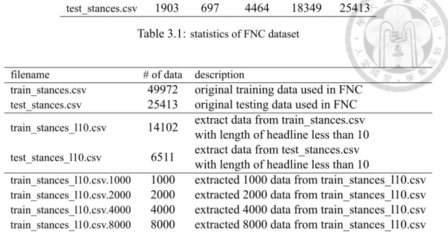
filename # of data description

train_stances.csv 49972 original training data used in FNC test_stances.csv 25413 original testing data used in FNC train_stances_l10.csv 14102 extract data from train_stances.csv

with length of headline less than 10 test_stances_l10.csv 6511 extract data from test_stances.csv

with length of headline less than 10

train_stances_l10.csv.1000 1000 extracted 1000 data from train_stances_l10.csv train_stances_l10.csv.2000 2000 extracted 2000 data from train_stances_l10.csv train_stances_l10.csv.4000 4000 extracted 4000 data from train_stances_l10.csv train_stances_l10.csv.8000 8000 extracted 8000 data from train_stances_l10.csv

Table 3.2: preprocessing of FNC dataset

3.2 Adversarial Examples

It was [16] that first proposed the term“adversarial examples”. They found that applying a imperceptible perturbation to an image may change the classifier’s prediction. Also, researchers tries to find out the reason why some models are vulnerable to adversarial examples. In [7], the authors thought that the cause to adversarial examples may be the linear behavior in high-dimensional spaces.

In our work, we define the adversarial examples in FNC classification task as changing at most one word in the headline. To be more specific, for each headline-body pair in training data, we try to revise the headline by changing a word into an unknown token

”<unk>”. Later, let the model to predict the label of this new headline-body pair to see if it would predict a label different from its previous prediction. If the new label is different from the original one, we regard this new headline-body pair as an adversarial example toward the given black-box classifier model.

Notice that we only change at most one word into a unknown token because we want to most likely preserve the meaning between the original data and the syntactic data. That is, given a sentence s = (w₁, w₂, …, w_T) with length T , a syntactic sentence

6

s^′ = (w₁^′, w^′₂, …, w_T^′ ) is a valid adversarial example if and only if∑_T

t=1Jwt ̸= w^′tK ≤ 1 whereJ·K equals to 1 if the statement is true, otherwise is 0.

3.3 Adversarial Training

[16] found that training a new model on direct combination of adversarial examples and original training data could bring an improvement. Researchers from [7] did adversarial training with a new objective function utilizing the fast gradient sign method they pro- posed. Under their setting, the adversarial examples keep changing between each itera- tion, and they think that it could let the training algorithm focus on adversarial examples corresponding to the current vision of the model.

In this work, we simply train a new classifier by the original training objective function, but we use the new training data instead. Similar to [7], we obtain the new training data by combining the original headline-body pairs and its adversarial examples. The detail will be discuss in section 4.5.

doi:10.6342/NTU201802182

Chapter 4 Model

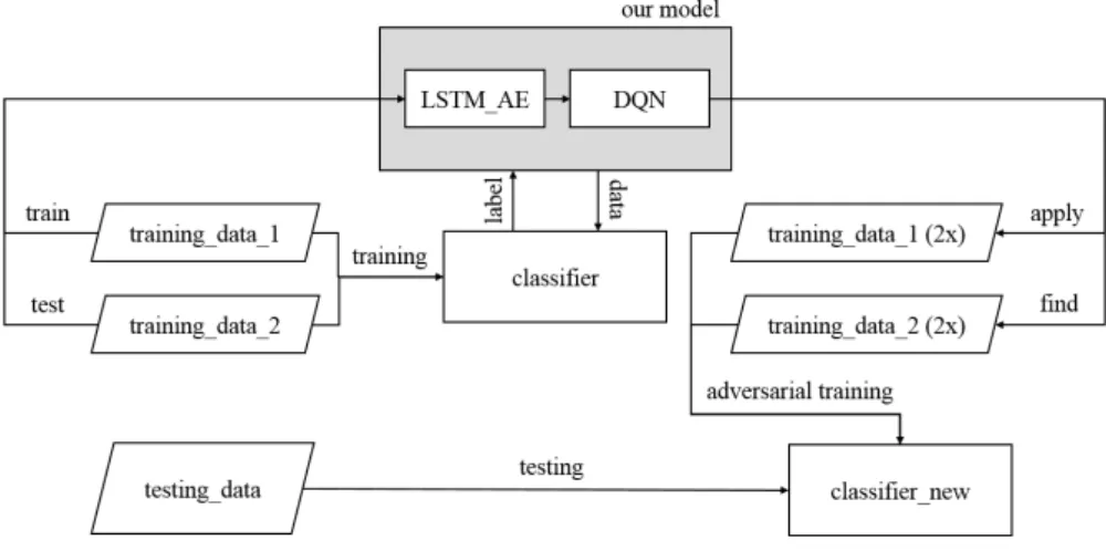
Our model consists of four parts: the baseline classifier, LSTM autoencoder, reinforce- ment learning environment, and deep Q network (DQN). Figure 4.1 is the flowchart of our model. We discuss the detail of each component in the following sections.

4.1 Baseline Classifier

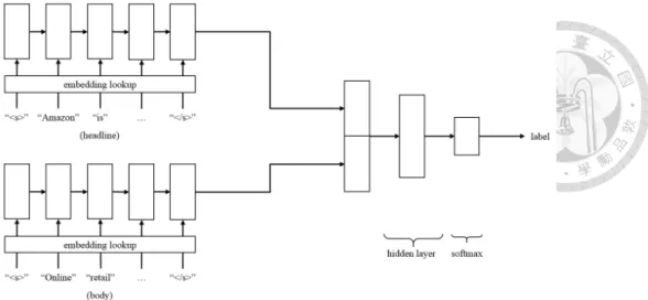
Given a black-box classifier, our model needs to find adversarial examples that this given classifier would predict wrong labels to them. For the reason that this classifier is a black box in our scenario, we could get nothing more information but the probability it predicts to our given input data. In our experiments, we implement a simple LSTM-RNN classifier as the target black-box model. Figure 4.2 is the architecture of our classifier. It uses two

Figure 4.1: Flowchart of our model

8

Figure 4.2: LSTM-RNN Classifier Model

distinct LSTM-RNN to encode input headlines and bodies into two embeddings. We keep the most frequency top|V | vocabularies, which is 20000 in our setting, and change all out of vocabularies into a unknown token <unk>. Next, the output states of these two LSTM- RNN are concatenated and served as the input of a fully connected two-layer network. The dimension of the two hidden layers is set to 100 and 200. Finally we add the output layer with dimension as the number of predict labels, which is 4 in the FNC dataset. We also implement early stopping and dropout technique [13] in each hidden layer with dropout rate set to 0.5.

Though we only carry out experiments on a simple LSTM-RNN classifier, it is easily to apply our finding framework to any black-box classifier to find corresponding adversarial examples. This is because our model is in black-box attack scenario, any classifier with interface of input sentences and output labels could be applied in our framework.

4.2 LSTM Autoencoder

As the flowchart shown in the Figure 4.1, we need a function ϕ to map discrete sentence sequence into a continuous vector representation which could be served as the input of later DQN model. The idea of using a mapping function to represent a sentence into a continuous vector could be seen in many situations such as [8]. We use an encoder as the function in our experiment and pretrain it under sequence to sequence autoencoder

doi:10.6342/NTU201802182

framework. This pretrained way was proposed by [3] and they found that combining application with weight from pretrained autoencoder could have better performance then the situation with random initialized weight. Figure 4.3 is a overview of our autoencoder model. Here we use the encoder-decoder architecture. To be more specific, we use a bidirectional RNN as the encoder to process a discrete natural language sentence, and for the decoder part we use a simple one directional RNN. Here we also use the LSTM as the RNN cell.

In our autoencoder model, we have a embedding lookup table to convert discrete words into continuous vectors for LSTM inputs. And this embedding is trained with the encoder- decoder simultaneously. We use the last hidden state from the encoder RNN as the ini- tialization of the decoder RNN. Because we use a bidirectional RNN as the encoder, we concatenate the output state from LSTM cells in both two direction as the initialization of decoder. In decoder, the hidden state of LSTM cell from each time step is connected to a softmax layer to calculate the probability of each predicted word:

p_t= softmax(h^de_t ),

where h^de_t is the hidden state in decoder in time step t, and p_t ∈ R^{|V |}. The goal of the decoder RNN is to reconstruct the original input sentence s = (w₁, w₂, …, w_T) by min- imizing the cross entropy between the softmax output and the true label. To be more

10

specific, the training process is to minimize the following function:

1

|S|

∑

s∈S

loss(s),

here S is the set consisting of all sentences in training data. And loss(s) here is the cross entropy of reconstructing a given sentence s:

loss(s) =

T−1

∑

t=1

CE(pwt+1, pt)

where p_wt+1 is a one-hot vector with 1 in the dimension representing word w_t+1.

We set |V | as 20000, and both embedding size and RNN state size as 300. The max- imum length T of RNN is set to 32. For each input sentence we add a starting token <s>

and a ending token </s> to the two endpoints of the sentence. We pretrain our autoencoder model by both headline sentences and body sentences in the training data for 20 epoch.

Then its weights are fixed during the training and testing of the DQN.

It’s believed that if the decoder could reconstruct the encoder’s input well, there may be some necessary information in the latent vector used for initialization of decoder.

We then use this encoder to map discrete sentences into continuous embedding that could be used in the reinforcement learning environment.

4.3 Reinforcement Learning Environment

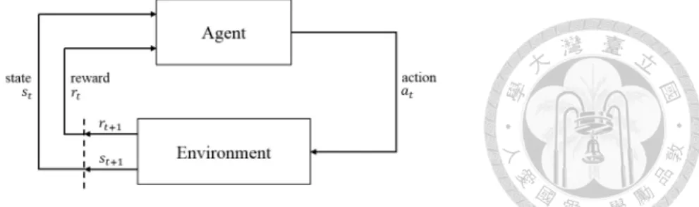
In a common reinforcement learning setting there should be an ”agent” that interacts with

”environment”. Each iteration the ”environment” gives the current ”state”, and the agent needs to make an ”action”. After that ”environment” gives a ”reward” and a new ”state” to

”agent” for next iteration. Figure 4.4 is an illustration of this interaction in reinforcement learning according to [15].

In our work, the ”state” is defined as the information of headline-body pair and the

”action” is defined as one of {<unk>, <pass>}. The action <unk> is to change a word into a unknown token <unk>, while <pass> does nothing. One problem is that the discrete

doi:10.6342/NTU201802182

Figure 4.5: State Representation of FNC data

natural language sequences are inconvenient for the later Q network, so here we utilize the LSTM autoencoder mentioned in section 4.2 as a mapping function ϕ which generates a continuous fixed-dimensional vector as state representation for a given state. To decide which word will be applied the action, we define a cursor that points to a word of the sentence. Figure 4.5 is our designed representation of state s. It consists of four 300 dimensional embeddings, totally results in a 1200 dimension vector. Assume that the cursor is now at the word w_t of headline, then the first part (s[:300]) is the

⇀

t−1 vector from the encoder given the headline sentence as input. Second part (s[300:600]) is the embedding of word that pointed by the cursor. Third part (s[600:900]) is the

↼

t+1 vector from the encoder. The last part (s[900:1200]) is the embedding of the body sentence and we just use

⇀

T from the encoder in our experiment. Here T is the length of the input sentence.

Now we give the analogy between the reinforcement learning framework and our clas- sification task. According to [15], there are some main elements of a reinforcement learn- ing system: ”policy”, ”reward function”, and ”value function”. The policy we need to learn in our experiment is to predict if changing the word currently pointed by the cursor will leads to an adversarial example. It will gives probabilities of the two action <unk>

12

and <pass>. Next we define the ”reward function” as the following

r =













1, action=<unk> and get adversarial example pori− padv − rp, action=<unk> but no adversarial example 0, action=<pass>

(4.1)

where rp is the penalty term with action <unk>. This is because the goal of our model is to find adversarial examples with as few as trails as possible, we add a penalty mechanism being as the cost of action <unk>. And the term pori and padv represent the predicted probability on true label from clean data and adversarial one, correspondingly. The next state that environment will give to agent is the same as the current state but with cursor right shifted one word, letting the model to learn if it is good to revise other words. That means no matter the agent selects action <unk> or not, the new state will always resume the original headline sentence, so that it meets the constraint that there are at more one revised word. For ”value function” here, we learn the state-action value. When given a state during inference, we just pick the action that could leads the greatest state-action value. Through the reinforcement learning process our model could lead the cumulative reward of each state and each action.

Another thing should be noticed is that we only take a portion of training data (ratio r_split) to train our DQN model, as shown in Figure 4.1. We test for different r_splitand try to find which setting is more effective. The result will be discussed in section 5.1.

4.4 Deep Q Network

[11] has shown how to use a deep neural network to learn the Q value. They applied their model on atari games and reached even better performance than human in some games.

In our work, the architecture of our Q network is shown in Figure 4.6. We concatenate the input state with a hidden layer with 128 dimension. Our Q-learning algorithm, shown in Algorithm 1, is heavily based on the learning algorithm in [11]. The main different

doi:10.6342/NTU201802182

thing is that there is only one starting state for each atari game, while there are many data and they could be different starting states in our scenario. In our algorithm, we train our deep Q network for M episode. In each episode, we feed all sentences with cursor pointing to the first word as initialized state. During the moving of the cursor to the last word, it keeps adding the transition (s_t, a_t, r_t+1, s_t+1) to the replay memory. The setting of memory queue is also different from the atari one. We find that the probability of sampling the transition with r_t+1 = 1 is low when we use the original setting, which leads to a slow learning process. So we change the setting into two independent memory queue D_hitand Dmiss. One for transitions with rt+1= 1, and the other one for other transitions.

After it finishes observing a whole sentence, it samples some transitions from both replay memory queue and train the DQN once. And it move to next sentence till the last one. Each time when we need to do memory replay to train our DQN, we sample half of batch size transitions from D_hit, and so does D_miss. We set the size of each replay memory N to 5000, sample batch size to 32, epsilon is initialized as 0.99, and decay of epsilon to 0.9. The total number of episode M is set to 40.

4.5 Adversarial Training

In our work, we also use the adversarial examples for testing whether combining original training data and adversarial examples could lead to a better performance. The amount of data in new training data will be double to the original data. Each sentence in original

14

Algorithm 1 Adversarial examples in FNC with deep Q-learning

1: Initialize replay memory D_hit, D_missto capacity N

2: Initialize action-value function Q with random weights

3: Initialize ϵ as 0.99

4: Initialize state representation function ϕ mentioned in section 4.3

5: for episode = 1, M do

6: Q^′ ← Q

7: for each headline-body pair in FNC dataset do

8: Initialize state s₁and preprocessed sequenced ϕ(s₁)

9: for t = 1,T do

10: With probability ϵ select a random action a_t

11: otherwise select a_t ← maxaQ^′(ϕ(s_t), a)

12: Execute action a_tand observe reward r_t+1and s_t+1

13: if r_t+1 = 1

14: Store transition (ϕ(s_t), a_t, r_t+1, ϕ(s_t+1)) in D_hit

15: else

16: Store transition (ϕ(s_t), a_t, r_t+1, ϕ(s_t+1)) in D_miss

17: end for

18: Sample minibatch (ϕ(s_j), a_j, r_j+1, ϕ(s_j+1)) from D_hitand D_miss

19: if terminal ϕ(s_j+1)

20: Set y_j ← rj+1

21: else

22: Set y_j ← rj+1+ γ max_a′Q^′(ϕ(s_j+1), a′)

23: Perform a gradient descent step on (y_j−Q(ϕ(s_j), a_j))²

24: end for

25: ϵ← ϵ ∗ 0.9

26: end for

doi:10.6342/NTU201802182

classifier and has an adversarial example, we replace the copied data to this adversarial example. In other words, there will be one clean sentence and one adversarial example in the new double-sized training data. Otherwise, if there are no adversarial examples of a sentence or it isn’t predicted correctly by the target classifier, there will be just two same original sentences. After having this double-sized training data, we could use it to train a new classifier.

16

Chapter 5 Experiments

In this chapter, we test our model in two orientation: adversarial examples and adversarial training. Besides, we try to modify the autoencoder part to see if it could bring better generalization. We will give discussions in each following section.

5.1 Adversarial Examples

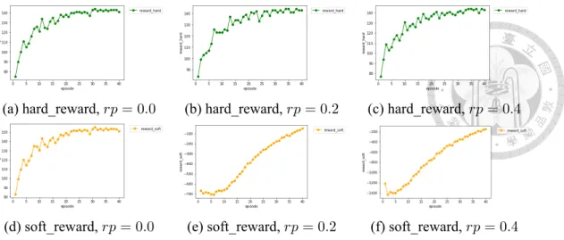
First, we test whether applying reward penalty rp in Equation 4.1 could really let our DQN predict the action leading to potential adversarial examples. We test for rp set to 0, 0.2, and 0.4, using data with size 1000. We plot the cumulative reward curve in Figure 5.1.

Here hard_reward counts the total rewards when finding adversarial examples (the first condition in Equation 4.1), while soft_reward is the summation of all rewards (all three conditions in Equation 4.1) in one episode. We could see that soft_reward is improving through the training process while keeping the number of adversarial examples it finds.

In other words, it improves the precision of predicting whether applying action <unk> on current word will lead to an adversarial examples. We calculate the precision, recall and F1-score (micro-F1) of our model on another data for testing and the result is in Table 5.1.

The last row here is greedily find all possible adversarial examples, but it has the lowest precision 0.0357. We find that 0.4 gives the highest F1-score so we use rp = 0.4 in the later experiments.

Next we evaluate whether our model could be trained by only a few parts of data.

doi:10.6342/NTU201802182

(d) soft_reward, rp = 0.0 (e) soft_reward, rp = 0.2 (f) soft_reward, rp = 0.4

Figure 5.1: Cumulative Reward Curve with Different rp

As mentioned in section 4.3, we split the training data by ratio r_split. The process is two stages: we use the r_splitpart to train DQN and 1−rsplitpart for testing DQN performance.

We test rsplit = 0.2, 0.4, 0.6, and 0.8 in four data with different scales. The performance in both two stages could be found in Figure 5.2. Here we report the average cost (trials) our DQN needs to find an adversarial example. This number is related to success rate, i.e.

lower cost means a more efficient way of finding. We report the precision in three stages:

DQN training stage (“apply”in Figure 4.1), inference stage (“find”in Figure 4.1), and the average of previous two stages. We find that in all four different scales of data, the best precision exists when r_split is set to 0.2. This is surprising that only a small portion of data is enough to train a effective finding model that perform well on the left 1− rsplit

portion, although some adversarial examples would be missed in the second stage. We also find that the precision is becoming better when the scale of data is becoming larger.

The result shows that when the amount data is 8000, using 20% of data to train our DQN and using trained network to predict on the left 80% data could lead to 16.38 average cost, while greedily revising all words leads to 29.44. It shows that our DQN and rein- forcement learning framework could actually benefit finding process. Especially when the cost to confirm with target classifier model is not negligible or the quota of confirming to the target classifier is limited, a finding process with better success rate could find more adversarial examples.

18

model rp precision recall F1-score DQN 0.0 0.0609 0.5490 0.1096 DQN 0.2 0.0830 0.4145 0.1383 DQN 0.4 0.0907 0.3709 0.1458

greedy - 0.0357 1 0.0690

Table 5.1: F1-score with Different rp

(a) data scale: 1000 (b) data scale: 2000

(c) data scale: 4000 (d) data scale: 8000

Figure 5.2: Precision in Two Stage with Different Scale of Data

5.2 Adversarial Training

We also test whether adversarial examples we find could help us train a better classifier by the same learning algorithm. Here we train the DQN with the parameter r_split set to 0.2. We combine the original data and adversarial examples by the method discussed in section 4.5. After obtaining the new data that is twice larger than the original one, we train a new classifier model on it by the same learning algorithm. The result of adversarial training is in Table 5.2. Here we report the average accuracy and standard deviation of five repeat experiments. In the result we find that adversarial training could improve the performance in three of four scales training data.

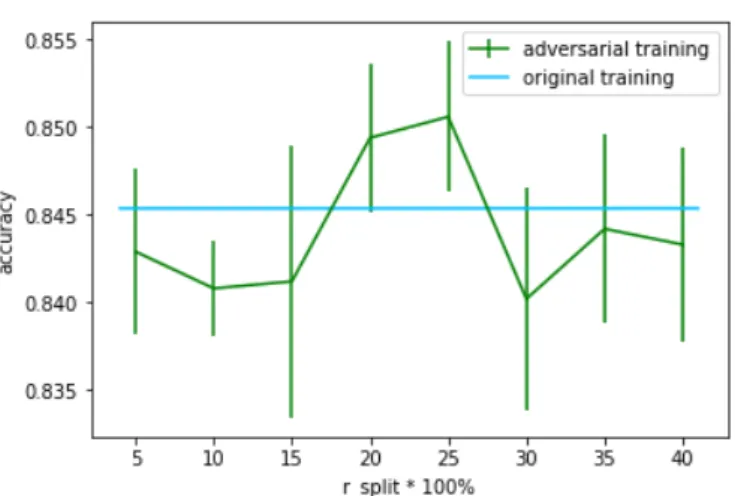
Besides the success on adversarial training with r_split set to 0.2, we want to know whether a smaller r_splitcould also brings benefit. We test for different r_split setting from 5% to 40%, and the result is in Figure 5.3 The result shows that not every adversarial

doi:10.6342/NTU201802182

train_stances_l10.csv.1000 0.8370 0.8337 train_stances_l10.csv.2000 0.8213 0.8399 train_stances_l10.csv.4000 0.8363 0.8417 train_stances_l10.csv.8000 0.8454 0.8494

Table 5.2: Result of Adversarial Training

Figure 5.3: Adversarial Training

training results are better than original accuracy. We find that our adversarial training setting only works when r_split is set to 20% and 25%. We also test for r_split = 100% (i.e.

find all adversarial examples by confirming with target model directly) and the result is not better than original training either. The reason why our adversarial training setting only works at r_split= 20% or 25% is not clear and it needs more further research.

5.3 Different State Representation

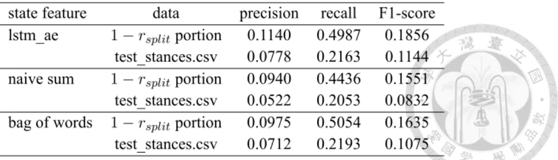
We also test our trained DQN on the data that both never seen before. That is, we test the performance of DQN on the testing data from FNC while our target classifier and DQN are trained on training data. The result is shown in Table 5.3. We could find that there is a performance gap between seen and unseen data. We initially think that this may be due to the complexity of state representation from RNN, so we also test other function such as naive sum and bag of words as the state representation in reinforcement learning. Although this is not a serious problem in FNC dataset because the high overlap of headline or body

20

state feature data precision recall F1-score lstm_ae 1− rsplitportion 0.1140 0.4987 0.1856

test_stances.csv 0.0778 0.2163 0.1144 naive sum 1− rsplitportion 0.0940 0.4436 0.1551 test_stances.csv 0.0522 0.2053 0.0832 bag of words 1− rsplitportion 0.0975 0.5054 0.1635 test_stances.csv 0.0712 0.2193 0.1075

Table 5.3: Different State Representation

filename 美牛 基薪 自經 服貿 核四 total

raw_data 128 194 116 739 125 1302

train.csv 50 50 50 50 50 250

test.csv 50 50 50 50 50 250

Table 5.4: statistics and preprocessing of zhtNews dataset

sentences between the r_split and 1− rsplit parts, we guess the gap would be a problem when applying our model to other more sparse dataset and it needs further research.

5.4 Other Datasets

Besides the success in FNC dataset, we also try our model on other more general datasets.

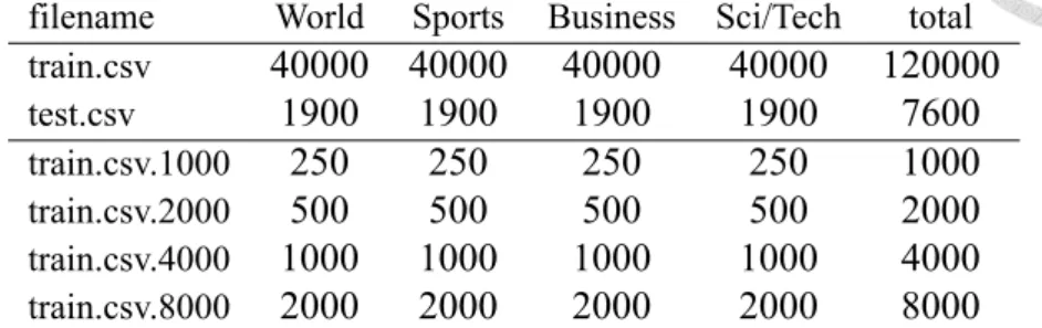
That is, the input is just one sentence instead of a headline-body pair. We apply our model on three more datasets: zhtNews, AG’s News and IMDB. zhtNews is a dataset collected by lab senior and Table 5.4 is its statistic. We find that applying data augmentation in this dataset could bring a better accuracy on unseen testing data, as shown in Table 5.5. AG’s News [17] is a dataset about News article and the statistics is in Table 5.6. We again extract some small scale subset from original training data. The result is in Table 5.7. We also find that adversarial training works on this dataset. We also test our framework on IMDB [9], an movie review dataset. The statistic and result is in Table 5.8 and Table 5.9 correspondingly. In this dataset adversarial training only works in only 1000 and 2000 scale training data.

doi:10.6342/NTU201802182

train.csv 0.7376 0.7720

Table 5.5: Result of Adversarial Training of zhtNews dataset

filename World Sports Business Sci/Tech total

train.csv 40000 40000 40000 40000 120000

test.csv 1900 1900 1900 1900 7600

train.csv.1000 250 250 250 250 1000

train.csv.2000 500 500 500 500 2000

train.csv.4000 1000 1000 1000 1000 4000

train.csv.8000 2000 2000 2000 2000 8000

Table 5.6: statistics and preprocessing of AG dataset

training file acc. w/o adv. acc. w/ adv.

train.csv.1000 0.5913 0.5922 train.csv.2000 0.6422 0.6623 train.csv.4000 0.6476 0.7041 train.csv.8000 0.7234 0.7398

Table 5.7: Result of Adversarial Training of AG dataset

filename pos neg total

train.csv 12500 12500 25000

test.csv 12500 12500 25000

train.csv.1000 500 500 1000 train.csv.2000 1000 1000 2000 train.csv.4000 2000 2000 4000 train.csv.8000 4000 4000 8000 Table 5.8: statistics and preprocessing of IMDB dataset

training file acc. w/o adv. acc. w/ adv.

train.csv.1000 0.5978 0.6332 train.csv.2000 0.6529 0.6622 train.csv.4000 0.6942 0.6877 train.csv.8000 0.7257 0.6953

Table 5.9: Result of Adversarial Training of IMDB dataset

22

Chapter 6 Conclusion

In this work, we apply reinforcement learning framework to find adversarial examples in text classification task. By applying a reward penalty, 0.4 in this work, our experiments show that it could actually lead to a efficient finding rate better than greedy baseline. Be- sides we propose a adversarial training setting to combine clean training data and adver- sarial examples. By training on the new data consisting of original data and adversarial examples we reach a better performance in all of our four scales data in FNC dataset.

Moreover we test for different portion used in training deep q network and find that the adversarial training performance is good while r_splitset to 0.2 or 0.25.

There are three potential direction of future works. One is extending the adversarial examples to semantic attack, that is, changing words into its synonyms instead of the un- known token. Although the computation complexity is larger then unknown-token attack, it might bring better performance in adversarial training phrase because the adversarial examples in this constraint will be closer to real data. Another research direction is the design of reward in reinforcement learning environment. Current adversarial training is two-stage: finding adversarial examples and then retraining classifier. The relationship is not clear between the adversarial examples we define and the benefit of adversarial train- ing. Whether it is possible to combine the improvement of adversarial training into the reward design is a potential research direction. The third one is the limit of distribution of data. Currently there is a performance gap between seen and unseen data. It would be better if the model could be more general to unseen data.

doi:10.6342/NTU201802182

Bibliography

[1] Fake news challenge. http://www.fakenewschallenge.org, 2017.

[2] D. Bahdanau, K. Cho, and Y. Bengio. Neural machine translation by jointly learning to align and translate. arXiv preprint arXiv:1409.0473, 2014.

[3] A. M. Dai and Q. V. Le. Semi-supervised sequence learning. In Advances in neural information processing systems, pages 3079–3087, 2015.

[4] J. Ebrahimi, A. Rao, D. Lowd, and D. Dou. Hotflip: White-box adversarial examples for nlp. arXiv preprint arXiv:1712.06751, 2017.

[5] H. Guo. Generating text with deep reinforcement learning. arXiv preprint arXiv:1510.09202, 2015.

[6] S. Hochreiter and J. Schmidhuber. Long short-term memory. Neural computation, 9(8):1735–1780, 1997.

[7] C. S. Ian J. Goodfellow, Jonathon Shlens. Explaining and harnessing adversarial examples. arXiv preprint arXiv:1412.6572, 2014.

[8] M. Iyyer, V. Manjunatha, J. Boyd-Graber, and H. Daumé III. Deep unordered com- position rivals syntactic methods for text classification. In Proceedings of the 53rd Annual Meeting of the Association for Computational Linguistics and the 7th In- ternational Joint Conference on Natural Language Processing (Volume 1: Long Pa- pers), volume 1, pages 1681–1691, 2015.

[9] A. L. Maas, R. E. Daly, P. T. Pham, D. Huang, A. Y. Ng, and C. Potts. Learning word vectors for sentiment analysis. In Proceedings of the 49th Annual Meeting

24

of the Association for Computational Linguistics: Human Language Technologies, pages 142–150, Portland, Oregon, USA, June 2011. Association for Computational Linguistics.

[10] T. Miyato, A. M. Dai, and I. Goodfellow. Adversarial training methods for semi- supervised text classification. arXiv preprint arXiv:1605.07725, 2016.

[11] V. Mnih, K. Kavukcuoglu, D. Silver, A. Graves, I. Antonoglou, D. Wierstra, and M. Riedmiller. Playing atari with deep reinforcement learning. arXiv preprint arXiv:1312.5602, 2013.

[12] K. Narasimhan, T. Kulkarni, and R. Barzilay. Language understanding for text-based games using deep reinforcement learning. arXiv preprint arXiv:1506.08941, 2015.

[13] N. Srivastava, G. Hinton, A. Krizhevsky, I. Sutskever, and R. Salakhutdinov.

Dropout: a simple way to prevent neural networks from overfitting. The Journal of Machine Learning Research, 15(1):1929–1958, 2014.

[14] I. Sutskever, O. Vinyals, and Q. V. Le. Sequence to sequence learning with neural networks. In Advances in neural information processing systems, pages 3104–3112, 2014.

[15] R. S. Sutton, A. G. Barto, et al. Reinforcement learning: An introduction. MIT press, 1998.

[16] C. Szegedy, W. Zaremba, I. Sutskever, J. Bruna, D. Erhan, I. Goodfellow, and R. Fer- gus. Intriguing properties of neural networks. arXiv preprint arXiv:1312.6199, 2013.

[17] X. Zhang, J. Zhao, and Y. LeCun. Character-level convolutional networks for text classification. In Advances in neural information processing systems, pages 649–

657, 2015.