半導體廠金屬蝕刻機台於預防保養時之空氣污染物逸散控制研究

全文

(1)國立交通大學環境工程研究所. 碩士論文. 半導體廠金屬蝕刻機台於預防保養時之空氣污染物逸散控制研究. Research on the Control of Air Pollutant Dispersion during Preventive Maintenance of a Metal Etcher in a Semiconductor Factory. 研究生 : 簡誌良指導教授 : 蔡春進. 博士. 中華民國九十五年七月.

(2) 半導體廠金屬蝕刻機台於預防保養時之空氣污染物逸散控制研究 Research on the Control of Air Pollutant Dispersion during Preventive Maintenance of a Metal Etcher in a Semiconductor Factory. 研究生：簡誌良. Student: Chih-Liang Chien. 指導教授：蔡春進博士. Advisor: Chuen-Jinn Tsai, Ph.D.. 國立交通大學環境工程研究所碩士論文. A Thesis Submitted to Institute of Environmental Engineering College of Engineering National Chiao Tung University in Partial Fulfillment of the Requirements for the Degree of Master in Environmental Engineering July 2006 Hsinchu, Taiwan, Republic of China. 中華民國九十五年七月.

(3) 半導體廠金屬蝕刻機台於預防保養時之空氣污染物逸散控制研究學生：簡誌良. 指導教授：蔡春進博士國立交通大學環境工程研究所碩士班摘要. 半導體金屬蝕刻製程主要使用氯氣及氯化硼等氣體，以高能電漿離子化產生自由基後使其與晶圓表面之鋁反應將多餘之鋁蝕刻而產生溝槽。為維持晶圓生產良率須定期進行腔體的預防維護保養，主要清除反應腔壁所附著製程副產物，在此過程中在打開密閉反應腔及擦拭腔壁時會產生極刺鼻味道且含有毒性氣體，會逸散至潔淨室，造成勞工健康危害並汙染製程。本研究之主要目的在於利用數值模擬方法研究應用材料公司 P5000 金屬蝕刻機台於預防保養時的空氣污染物逸散控制方法與控制效率。前人曾以 1000 ppm 的追蹤氣體 SF6 在腔底連續釋放，測試反應腔上方有氣罩或反應腔上方無氣罩時的在側邊大量抽氣(3130 L/min)的控制效率，本研究則利用數值模擬方法驗證實驗數據，並探討側邊抽氣流率改變時對空氣污染物逸散的控制效率。研究結果顯示，不論反應腔上方全開(無氣罩)或上方有氣罩時在反應腔上方進行大量抽氣，可有效地控制危害性氣體的逸散，模擬的控制效率結果與實驗數據相符合，且發現在人員呼吸帶的 SF6 濃度均低於 FTIR 之偵測下限。當側邊抽氣流率降低但仍維持在一定流量以上時，空氣污染物的逸散仍可有效的獲得控制，而反應腔上方有氣罩時的控制效率會優於無氣罩時的控制效率。. I.

(4) Research on the Control of Air Pollutant Dispersion during Preventive Maintenance of a Metal Etcher in a Semiconductor Factory Student：Chih-Liang Chien. Advisors: Chuen-Jinn Tsai, Ph.D.. Institute of Environmental Engineering National Chiao Tung University ABSTRACT Main process gases used in the metal etcher of the semiconductor industry are chlorine and boron chloride. Process gases are ionized in the reactor chamber to form free radicals by plasma, which etches off aluminum film from the wafer surface. To increase the product yield, by-products deposited on the chamber wall must be cleaned periodically during preventive maintenance. As the chamber is being cleaned, toxic gases are released which may disperse in the clean room posing heath threat to workers, contaminate process tool, and create wafer defects. The main objective of this study is to use the numerical model to investigate the control method of pollutant dispersion and its control efficiency for a type P5000 metal etcher of Applied Materials Inc. during preventive maintenance. In previous work, sulfur hexafluoride (SF6 ) tracer gas of 1000 ppm was released at different flow rates at the chamber bottom to evaluate the control efficiency of the chamber with the hood at the chamber top, or without the hood by side venting at a large flow rate of 3130 L/min. Numerical results of the control efficiency were verified with the experimental data at the large venting flow rate. The control efficienc y of side venting at different flow rates was also investigated. Results show that pollutant dispersion of a metal dry etcher during preventive maintenance can be effectively controlled by side venting at a large flow rate near the chamber top whether the chamber is fully open (without the hood) or with the hood. Good agreement between the experimental data and the simulation results is obtained. The SF6 concentration at the breathing zone was also found to be lower than the detection limit of the FTIR spectrometer. When the side venting flow rate is reduced but maintaining above a fixed value, the pollutant dispersion still can be effectively controlled, and the control efficiency of the chamber with the hood is superior to that of the chamber without the hood. II.

(5) Contents Abstract (Chinese)… … … … … … … … … … … … … … … … … … … … … … .... I. Abstract (English)… … … … … … … … … … … … … … … … … … … … … … …. II. Contents… … … … … … … … … … … … … … … … … … … … … … … … … … .... III. List of tables… … … … … … … … … … … … … … … … … … … … … … … … … .. V. List of figures… … … … … … … … … … … … … … … … … … … … … … … … ... VI Nomenclature… … … … … … … … … … … … … … … … … … … … … … … … ... IX. Chapter 1 Introduction… … … … … … … … … … … … … … … … … … … … .... 1. 1.1 Toxicity originated from waste gases of the metal etcher… … … .. 1. 1.2 FTIR application in clean room… … … … … … … … … … … … … .. 2. 1.3 Control efficiency of hood… … … … … … … … … … … … … … …. 2. 1.4 Objectives of this study… … … … … … … … … … … … … … … … .. 3. Chapter 2 Experimental methods… … … … … … … … … … … … … … … … .... 4. 2.1 Experimental system… … … … … … … … … … … … … … … … … .. 4. 2.2 Control efficiency… … … … … … … … … … … … … … … … … … ... 5. Chapter 3 Numerical methods… … … … … … … … … … … … … … … … … …. 10. 3.1 Governing equations… … … … … … … … … … … … … … … … … .. 10 3.2 Turbulence model… … … … … … … … … … … … … … … … … … .. 10 3.3 Wall functions… … … … … … … … … … … … … … … … … … … .... 11. 3.4 Mass sink… … … … … … … … … … … … … … … … … … … … … .... 12. 3.5 CFD modeling… … … … … … … … … … … … … … … … … … … .... 13. 3.6 Boundary conditions… … … … … … … … … … … … … … … … … .. 14. III.

(6) 3.7 Rotating reference frames… … … … … … … … … … … … … … … .. 15. 3.8 Control efficiency… … … … … … … … … … … … … … .................. 15 Chapter 4 Results and discussions… … … … … … … … … … … … … … … … .. 22. 4.1 Simulated airflow field and concentration field (case 1)… … … ... 22. 4.2 Comparison between experimental data and simulation results (case 1)… … … … … … … … … … … … … … … … … … … … … … ... 22. 4.3 Simulated airflow field and concentration field (case 2)… … … ... 23. 4.4 Comparison between experimental data and simulation results (case 2)… … … … … … … … … … … … … … … … … … … … … … ... 24. 4.5 Simulated airflow field and concentration field at different venting flow rates (case 1)… … … … … … … … … … … … … … …. 25. 4.6 Simulation results at different venting flow rates (case 1)… … …. 26. 4.7 Simulation results at different venting flow rates (case 2)… … …. 27. Chapter 5 Conclusions… … … … … … … … … … … … … … … … … … … … .... 57. Reference … … … … … … … … … … … … … … … … … … … … … … … … … ... 58 Appendix … … … … … … … … … … … … … … … … … … … … … … … … … ... 61. IV.

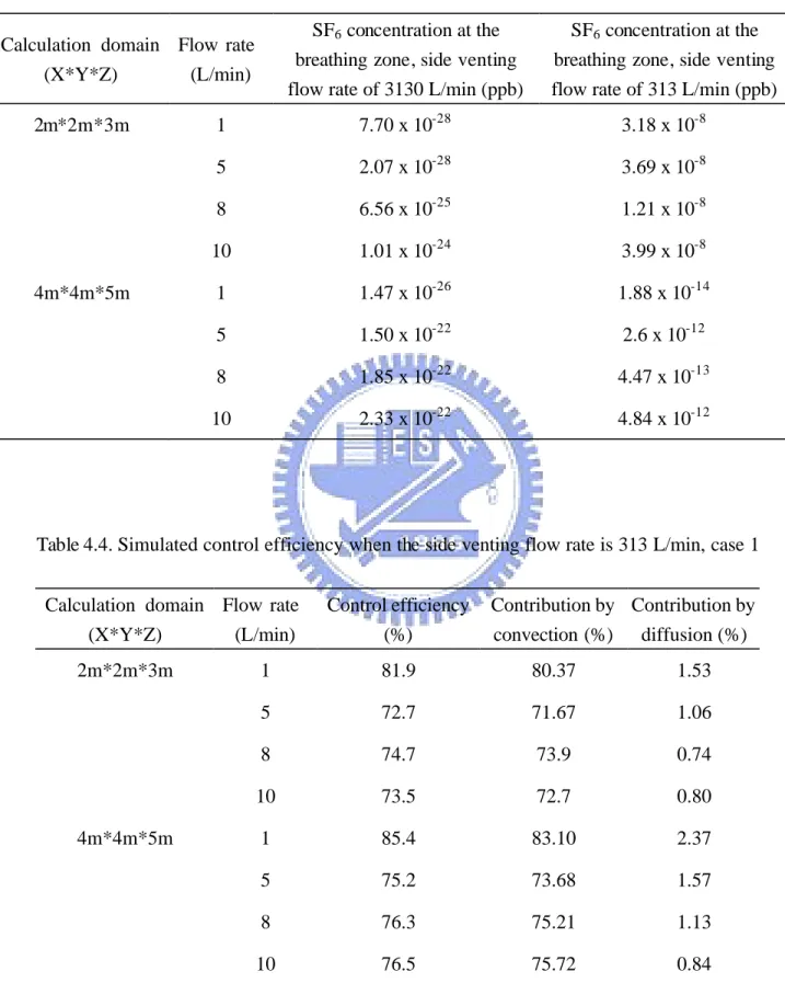
(7) List of tables Table 3.1 Information of mass sink… … … … … … … … … … … … … … … .... 17. Table 3.2 Size of calculation domains and grids used for simulation… … .... 17. Table 3.3 Inlet flows at the opening of each gas distribution tube… … … …. 17. Table 4.1 Experimental data under different conditions when the side venting flow rate is 3130 L/min (Ku, 2004)… … … … … … … … .. 29 Table 4.2 Simulated control efficiency when the side venting flow rate is 3130 L/min, case 1… … … … … … … … … … … … … … … … … …. 29. Table 4.3 Simulated SF6 concentration at the breathing zone when the side venting flow rate is 3130 L/min or 313 L/min, case 1.… … … … .. 30. Table 4.4 Simulated control efficiency when the side venting flow rate is 313 L/min, case 1… … … … … … … … … ..… … … … … … … … …. V. 30.

(8) List of figures Fig 2.1 Chamber configuration of a metal etcher… … … … … … … … … ... 7. Fig 2.2 Chamber configuration of a metal etcher with a designed cover.... 8. Fig 2.3 Schematic diagram of the setup for evaluating the control efficiency of the ventilation system… … … … … … … … … … … .... 9. Fig 3.1 Sink region at the side window… … … … … … … … … … … … … .. 18 Fig 3.2 Mesh scheme of the chamber… … … … … … … … … … … … … …. 19. Fig 3.3 Mesh scheme of the chamber with a designed cover… … … … … . 21 Fig 4.1 Velocity vector for SF 6 release flow rate of 10 L/min, venting flow rate of 3130 L/min in the 2x2x3m domain, case 1… … … …. 31. Fig 4.2 Concentration distribution for SF 6 release flow rate of 10 L/min, venting flow rate of 3130 L/min in the 2x2x3m domain, case 1... 32. Fig 4.3 Measurements and simulated control efficiency of SF6 versus total gas flow rate when the side venting flow rate is 3130 L/min, case 1… … … … … … … … … … … … … … … … … … … … .. 33 Fig 4.4 Concentration distribution at the breathing zone for SF6 release flow rate of 10 L/min, venting flow rate of 3130 L/min in the 2x2x3m domain, case 1… … … … … … … … … … … … … … … … .. 34 Fig 4.5 Velocity vector of the chamber with the hood for SF 6 release flow rate of 10 L/min, venting flow rate of 3130 L/min in the 2x2x3m domain, case 2… … … … … … … … … … … … … … … … .. 35 Fig 4.6 Concentration distribution of the chamber with the hood for SF 6 release flow rate of 10 L/min, venting flow rate of 3130 L/min in the 2x2x3m domain, case 2… … … … … … … … … … … … … … …. VI. 36.

(9) Fig 4.7 Measurements and simulated control efficiency of SF6 versus total gas flow rate when the side venting flow rate is 3130 L/min, case 2… … … … … … … … … … … … … … … … … … … … .. 37 Fig 4.8 Velocity vector for SF 6 release flow rate of 10 L/min, venting flow rate of 313 L/min in the 2x2x3m domain, case 1… … … … ... 38. Fig 4.9 Concentration distribution for SF 6 release flow rate of 10 L/min, venting flow rate of 313 L/min in the 2x2x3m domain, case 1… .. 39. Fig 4.10 Velocity vector for SF 6 release flow rate of 10 L/min, venting flow rate of 0 L/min in the 2x2x3m domain, case 1… … … … … ... 40. Fig 4.11 Concentration distribution for SF 6 release flow rate of 10 L/min, venting flow rate of 0 L/min in the 2x2x3m domain, case 1… … .. 41. Fig 4.12 Simulated control efficiency of SF6 versus total gas flow rate when the side venting flow rate is 1565 L/min, case1… … ...… …. 42. Fig 4.13 Simulated control efficiency of SF6 versus total gas flow rate when the side venting flow rate is 313 L/min, case 1… … … … …. 43. Fig 4.14 Simulated control efficiency of SF6 versus total gas flow rate when the side venting flow rate is 156.5 L/min, case1… … … … .. 44 Fig 4.15 Simulated control efficiency of SF6 versus total gas flow rate when the side venting flow rate is 93.9 L/min, case 1… … … … ... 45 Fig 4.16 Simulated control efficiency of SF6 versus total gas flow rate when the side venting flow rate is 31.3 L/min, case 1..… ............. 46 Fig 4.17 Simulated control efficiency of SF6 versus total gas flow rate when the side venting flow rate is 4695 L/min, case 1..… … … …. 47. Fig 4.18 Simulated control efficiency of SF6 versus different side venting flow rates when SF6 release flow rate is 10 L/min, case1… … … .. 48 Fig 4.19 Simulated control efficiency of SF6 versus different side venting flow rates when SF6 release flow rate is 8 L/min, case1… … … …. 49. Fig 4.20 Simulated control efficiency of SF6 versus different side venting flow rates when SF6 release flow rate is 5 L/min, case1… … … … VII. 50.

(10) Fig 4.21 Simulated control efficiency of SF6 versus different side venting flow rates when SF6 release flow rate is 1 L/min, case1… … … …. 51. Fig 4.22 Velocity vector of the chamber with the hood for SF 6 release flow rate of 10 L/min, venting flow rate of 313 L/min in the 2x2x3m domain, case 2… … … … … … … … … … … … … … … … .. 52 Fig 4.23 Concentration distribution of the chamber with the hood for SF 6 release flow rate of 10 L/min, venting flow rate of 313 L/min in the 2x2x3m domain, case 2… … … … … … … … … … … … … … …. 53. Fig 4.24 Simulated control efficiency of SF6 versus total gas flow rate when the side venting flow rate is 313 L/min, case 2… … … … …. 54. Fig 4.25 Velocity vector of the chamber with the hood for SF 6 release flow rate of 10 L/min, venting flow rate of 0 L/min in the 2x2x3m domain, case 2… … … … … … … … … … … … … … … … .. 55 Fig 4.26 Concentration distribution of the chamber with the hood for SF 6 release flow rate of 10 L/min, venting flow rate of 0 L/min in the 2x2x3m domain, case 2… … … … … … … … … … … … … … … … .. 56. VIII.

(11) Nomenclature A. cross section area. Aout. area at outlet cross section. C. concentration. Γf. associated diffusion and source coefficients. CE. control efficiency. D. diffusion coefficient. dij. Kronecher delta. E. empirical coefficient. J. diffusion flux. ?. von Karman constant. •. m •. min •. m out •. m sin k. mass flow rate of the injected/extracted stream per unit volume mass flow of inlet mass flow rate of outlet by convection mass flow rate of sink. µ. molecular dynamic fluid viscosity. µe. effective viscosity. µt. turbulent viscosity. P. sub-layer resistance factor. p. ensemble average pressure. ρ. density. ?air. air density. IX.

(12) Q. venting flow rate. Qin. inlet flow rate. Qout. outlet flow rate. sij. rate of strain tensor. sf. associated diffusion and source coefficients. sφ. molecular Prandtl number. sφ ,t. turbulent Prandtl number. τij. stress tensor component. Ud. venting velocity. u. fluid velocity vector. ui. ensemble average velocity in direction xi. Vout. velocity at outlet cross section. Vd. removal volume. x. distance. xi. Cartesian coordinate. f. dependent variables. Y. mass fraction of species. [ Yin ]kg / m. 3. mass concentration of species at the inlet in kg/m3. y+. dimensionless normal distance from the wall. ym+. cross-over point between the viscous sub-layer and the logarithmic region. ψ. mass fraction. X.

(13) Chapter 1 Introduction Main process gases used in the metal etcher of the semiconductor industry are chlorine and boron chloride. Process gases are ionized in the reactor chamber at a pressure below 1 torr to form free radicals by plasma, which etches off aluminum film from the wafer surface. To increase the product yield, by-products deposited on the chamber wall must be cleaned periodically during preventive maintenance, when the reaction chamber is opened and de-ionized water or isopropyl alcohol (IPA) is applied to clean up the chamber wall. As the chamber is being cleaned, toxic gases are released which may disperse in the clean room posing heath threat to operators.. 1.1 Toxicity originated from waste gases of the metal etcher The toxicity of waste gases, contaminated vacuum oils, and solid debris originated from the metal etcher has been studied in the acute oral and subchronic inhalation tests with laboratory rats by many previous investigators. Bauer et al. (1992) exposed rats to exhaust gas of a plasma etcher and found statistically significant increases in chromosomal aberrations and sister chromatid exchanges in bone marrow cells. Schmidt et al. (1995) found that pregnant mice suffered from prenatal toxic effects when treated with solid waste products originated from aluminum plasma etching processes. For rats fed with contaminated vacuum oil from a plasma etcher, all the ir livers showed hypertrophic degenerations. And clear genotoxic effects caused by the contaminated oil samples were observed in the Ames assay and Micronucleus assay (Bauer et al., 1995). Bauer et al. (1996) concluded that waste produc ts from plasma etching process had clear genotoxic, embryotoxic, and teratogenic effects that could be demonstrated as chromosomal aberrations, micronuclei, sister chromatid exchanges, embryo lethality, fetal developmental retardation, and spontaneous abortions. Muller et al. (2002). 1.

(14) studied the genotoxicological characterization of a complex mixture of mostly perhalogenated hydrocarbons generated as waste products from plasma etching process by use of tests in human cell types (lymphocytes and normal bronchial epithelial cells) and in rat hepatocytes. Results showed that the mixture acted as direct genotoxicant and there was no detoxification by the external enzyme system.. 1.2 FTIR application in clean room An extractive Fourier transform infrared (FTIR) spectrometer was successfully used to locate, identify, and quantify the odor sources inside the clean room of a semiconductor manufacturing plant (Li et al., 2003). The FTIR spectrometer was used to monitor the potential hazardous gas emission during preventive maintenance of a metal etcher. Toxic gases such as HCl, HCN, CCl4, HCOOH, CO, and IPA etc. were detected by the FTIR spectrometer and found to release into the clean room during preventive maintenance of a metal etcher, with the peak concentrations of 195, 220, 5.4, 5.18, 5.93, and 464 ppm (Chang et al., 2000).. 1.3 Control efficiency of hood Because of the release of potential toxic gases, workers normally wear full- face breathing respirator as a standard operation procedure during preventive maintenance. To further reduce the health risk of maintenance workers, it is very critical to control toxic gas dispersion during chamber cleaning. One of the effective ways to control toxic gas dispersion is by ventilation. In the literature, the gas tracer technique was used to evaluate the control efficiency of an industrial local exhaust hood (Hampl, 1984; Hampl et al., 1986), and laboratory fume hood (Ivany et al., 1989). In these studies, sulfur hexafluoride (SF6 ) was used as a tracer gas which was monitored by specific detectors. In addition, numerical simulations were used to evaluate 2.

(15) the control efficiency of the local exhaust/ventilation hood by calculating airflow and concentration fields (Kulmala, 1994; Kulmala, 1995; Kulmala, 1995; Kulmala et al., 1996; Heinonen et al., 1996; Kulmala, 2000). Although the numerical results were in satisfactory agreement with the experimental data, these studies only focused on the location of exhaust openings, the physical hood designs, and the use of local supply air. In the clean room of the semiconductor industry, the on-site testing results compared with the numerical solutions for the local ventilation hood are very limited. Both the local ventilation hood and the flexible house vacuum line appeared to be effective ways to prevent the toxic gas emission during preventive maintenance activities that may deteriorate the clean room air quality (Li et al., 2005).. 1.4 Objectives of this study In previous work, SF6 tracer gas was released at different flow rates at the chamber bottom to simulate gas pollutants generated during preventive maintenance. A FTIR spectrometer was used to measure the control efficiency and SF6 concentration near the breathing zone of workers. In this study, we evaluated the efficiency of controlling pollutant dispersion of a metal dry etcher by side venting at a large flow rate near the chamber top. Numerical results of the control efficiency were verified with the experimental data at the large venting flow rate. The control efficienc y of side venting for the chamber with or without the hood at different venting flow rates were also investigated by changing the mass flow rate of sink in the simulation.. 3.

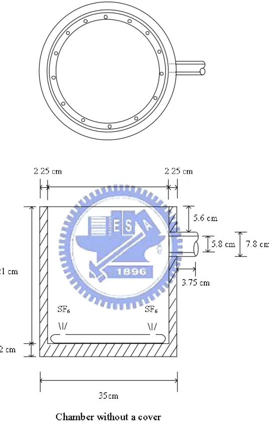
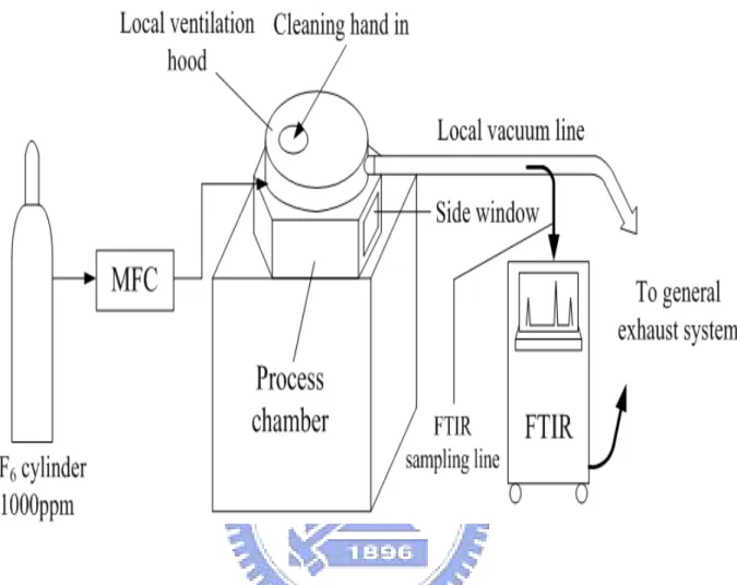
(16) Chapter 2 Experimental methods 2.1 Experimental system The experiment using a type P5000 metal etcher of Applied Materials Inc. was conducted in the earlier study (Ku, 2004). As shown in Fig. 2.1, the etcher has a cylindrical chamber (diameter: 30.5cm, depth: 21cm), and the distance from the chamber opening to the center of the sight window (diameter of the side window: 5.8cm) is 9.5 cm. The top of the chamber is about 122 cm in height from the clean room floor. Two cases were tested. In case 1, the chamber was open at the top and the gas was vented through the sight window via a low vacuum line (inner diameter: 3.8cm, outer diameter: 4.5cm, and length: 5.6m) near the opening at the flow rate of 3130±60 L/min. In case 2, the chamber was covered by an enclosed hood and shown in Fig. 2.2. At the top leaves a hole with 10 cm in diameter for the hand of a worker to access the chamber to mimic the chamber cleaning action. In this case, the gas was vented at the same flow rate near the top of the hood. For the purpose of preventive maintena nce, the workers can access the chamber by hands through the opening (diameter: 10cm, airflow velocity: 4.9m/s, and average flow rate of supply air: 2.31m3 /min) of the hood. The hood was also vented through the low vacuum line to control tracer gas dispersion. SF6 tracer gas of 1000 ppm was released for 5 minutes at the chamber bottom through a circular 1/4 inch PFA distribution tube with 14 holes of 2 mm in diameter while the gas was vented through the sight window (case 1, without a hood) or hood (case 2) via a low vacuum line in both cases. The control efficiency with a hood (case 2) was measured when the SF6 flow rate was 5 L/min, and the control efficiency without a hood (case 1) was measured at the SF6 flow rate of 1, 5, 8, and 10 L/min, respectively. Fig. 2.3 shows the schematic diagram of the setup for evaluating the control efficiency of. 4.

(17) the ventilation system (Li et al., 2005). The low vacuum venting line was connected with the chamber at the side window to control tracer gas dispersion without using the hood (case 1). The airflow velocity at the chamber opening (average flow rate of supply air: 2.54m3 /min) of the type P5000 metal etcher chamber was 0.58 m/s in average, and 0.65 m/s at the center. In case 2, we stretched hands into the chamber through the access hole to simulate the cleaning and wiping action during preventive maintenance. Also, the venting velocity through the low vacuum venting tube was 46±1 m/s at the flow rate of 3130±60 L/min. The vertical downward flow velocity of the clean room was 0.3 m/s. The height of the personnel breathing zone near the chamber was 150 cm from the clean room floor. The experimental data were obtained using Bomen FTIR (ABB Bomem, Canada), which was equipped a liquid-nitrogen detector and a gas cell with an optical path length of 10m. The infrared absorbance spectra were recorded over the frequency range of 500 cm-1 to 4500 cm-1 at a resolution of 1 cm-1 . The gas sample was introduced into the gas cell using a vacuum pump. The sampling flow rate was maintained at about 5 L/min, checked by a standard bubble meter, by monitoring the pressure drop of the sampling train. Details of FTIR experimental procedures and configurations were described in the earlier work (Li et al., 2003).. 2.2 Control efficiency The control efficiency in case 1 with a hood, CE1 , is defined as CE1 =. Cm1 ×100% Ci1. (2.1). where Cm 1 is the SF6 concentration in the low vacuum venting tube when the tracer gas is released at the bottom of the chamber, and Ci1 is the SF6 concentration in the low vacuum venting line when the tracer gas is introduced directly into the vacuum line. Similarly, the control efficiency in case 2 without using a hood, CE2 , is defined as. 5.

(18) CE2 =. Cm2 ×100% Ci 2. (2.2). where Cm 2 is the SF6 concentration in the low vacuum venting line when the tracer gas is released at the bottom of the chamber, and Ci2 is the SF6 concentration in the low vacuum venting line when the tracer gas is introduced into the vacuum line directly.. 6.

(19) Fig. 2.1. Chamber configuration of a metal etcher.. 7.

(20) Fig. 2.2. Chamber configuration of a metal etcher with a designed cover.. 8.

(21) Fig. 2.3. Schematic diagram of the setup for evaluating the control efficiency of the ventilation system (Li et al., 2005).. 9.

(22) Chapter 3 Numerical methods 3.1 Governing equations According to the characteristics of airflow in the clean room, steady state and incompressible flow with constant physical properties and temperature was assumed. The mass continuity equations and Reynolds-averaged Navier-Stokes equations were solved with turbulence closure provided by the standard k-ε turbulence model. The governing equations of airflow can be written as (STAR-CD version 3.22 methodology, 2004). ∂ ( ?u j ) = 0 ∂x j. (3.1). ∂ ∂p ?u jui − t ij ) = − ( ∂x j ∂xi. (3.2). In the above equations, the over bar denotes the ensemble averaging process. xi is Cartesian coordinate ( i = 1, 2, 3 ), ui is the ensemble average velocity in direction xi , p is the ensemble average pressure, and ρ is the mass density. τij is stress tensor component and can be written as. τ ij = 2µs ij −. 2 ∂u k µ δ − ρ u ′iu ′j 3 ∂xk ij. (3.3). where µ is molecular dynamic fluid viscosity and dij , the Kronecher delta, is unity when and zero otherwise. sij , the rate of strain tensor, is given by sij =. 1  ∂ui ∂u j + 2  ∂x j ∂xi.    . (3.4). 3.2 Turbulence model The standard k-ε turbulence model was applied to model the turbulent effects in this study. The equation of turbulence kinetic energy can be written as. 10.

(23) ∂ µ ∂k 2 ∂u ∂u ( ?u j k − e ) = µt Pt − ?e − ( µt i + ?k ) i ∂x j s k ∂x j 3 ∂xi ∂xi. (3.5). where µt is the turbulent viscosity and is defined as µt =. Cµ ? k 2. (3.6). e. and µe is the effective viscosity defined by µe = µ + µt. (3.7). The equation of turbulence dissipation rate is expressed as follows. ∂ µ ∂e e ( ?u j e − e ) = Ce1 ∂x j s e ∂x j k.  2 ∂ui ∂ui  e2 ∂u µ P − ( µ + ?k ) − C ? − Ce 3 ?e i  t t 3 t ∂x  e2 ∂xi  k ∂ xi  i. (3.8). where Cµ, Cε1, C ε2, C ε3, σk, σε, are empirical coefficients whose values are given below Cµ = 0.09, Cε1 = 1.44 , Cε2 = 1.92, Cε3 = 0.33, σk = 1.0, and σε = 1.22.. 3.3 Wall functions To make the simulation time economical, wall functions were used to resolve the near-wall flows in this study. Due to the damping effects of the wall surfaces in the near-wall region, the transport equations do not accurately represent the turbulence. Logarithmic law of wall functions concept is to extend the Couttee flow analysis and apply algebraic relations close to the near-wall region. The main idea of the wall functions approximation is based on that the flow in the near-wall region can be divided into three sub- layers, i.e. fully turbulent layer, buffer zone, and viscous sub-layer. Although the flow in the near-wall region comprises three zones, the wall functions approach assumes that the flow in the near-wall region can generally be divided into a fully turbulent layer and a viscous sub-layer. For standard wall functions formulae, the scaled velocity in terms of the normal distance from the wall can be expressed as below. 11.

(24)  y+  u = 1 +  ln( Ey ) κ +. y + < ym+ y + > ym+. (3.9). where y + is the dimensionless normal distance from the wall, ? is von Karman constant, E is empirical coefficient, and ym+ is the cross-over point between the viscous sub- layer and the logarithmic region. If ψ denotes mass fraction, then. φ + = sφ , t (u + + P). (3.10).  sφ 3 / 4   −0.007 sφ  P = 9.24  ( ) − 1 1 + 0.28exp( ) sφ ,t  sφ , t   . (3.11). where P is the sub- layer resistance factor， sφ is molecular Prandtl number, and sφ ,t is turbulent Prandtl number.. 3.4 Mass sink In STAR-CD, the differential equations governing the conservation of mass, momentum, and energy are discretised by the finite volume method. They are first integrated over the individual computational cells and then approximated in terms of the cell-center nodal values of the dependent variables. This approach has the merit of ensuring that the discretised forms preserve the conservation properties of the parent equations. General coordinate- free form of the conservation equations can be written as div ( ?uf − Γf gradf ) = sf. (3.12). where u is the fluid velocity vector, f stands for any of the dependent variables；and Γf , sf are the associated diffusion and source coefficients, respectively.. Local injection/extraction can be used anywhere within the mesh. The injection/extraction. 12.

(25) process is modeled as an additional source/sink term sf in the finite volume equation. The term is of the form •. sf = mf. (3.13). •. where m is the mass flow rate of the injected/extracted stream per unit volume. In order to simulate venting at the large flow rate at the side window (case 1) or from the hood (case 2), the mass sink was calculated by the user subroutine fluinj.f, as described in the appendix. The subroutine initiates fluid removal at specified cells and at a prescribed rate in •. units of kg/m3 /s. The mass flow rate of sink, m sin k , can be calculated as •. msin k = −. ρair ×U d × A Q = − ρair × Vd Vd. (3.14). where ?air is air density, Ud is venting velocity, A is cross section area, Q is venting flow rate, and Vd is removal volume. Fig. 3.1 shows the assumption for the sink region with a thickness of 0.3 cm in fluid at the low vacuum line. The overall process of setting up mass sink is described as follows. First, create a set of cells where mass sink is located. A separate cell type index number should be assigned to this set. Finally, insert appropriate code in the user subroutine fluinj.f to specify the mass flux removed for cells of the required type. The control efficiencies of side venting at different flow rates were investigated by changing the mass sink in the simulation. In addition to simulate venting at the flow rate of 3130 L/min as listed in Table 3.1, different sink flow rates were also simulated: 0, 31.3, 313, 1565, and 4695 L/min.. 3.5 CFD modeling The grids were generated as multi-blocked tetragon grids by using an automatic mesh 13.

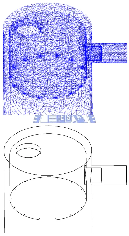
(26) generation tool, Pro-Modeler 2003 (CD-adapco Japan Co., LTD). Fig. 3.2 shows mesh scheme of the chamber with 14 sets of gas distribution tube which is 2 mm in diameter and 2 mm in height at the chamber bottom, and Fig. 3.3 shows mesh scheme of the chamber with a designed cover. The computational domain is 2m x 2m x 3m (393,000 grids) or 4m x 4m x 5m (799,000 grids). The maximum and the minimum length of mesh are 10 cm and 0.02 cm, respectively. The computational domains and the computational time are listed in Table 3.2. The above equations were solved using the STAR-CD 3.22 code (CD-adapco Japan Co., LTD), based on the finite volume discretization method. The estimation of diffusion fluxes at the cell faces was obtained by a centered approximation while upwind differencing was adopted for the convective fluxes. The pressure-velocity linkage was solved by the SIMPLE (semi- implicit method for pressure linked equation) algorithm (Patankar, 1972). A guessed pressure field was used to solve the momentum equations and a pressure correction equation derived from the continuity equation was solved to obtain a pressure correction field which was in turn used to update the velocity and pressure fields. The process was iterated until convergence of the velocity and pressure fields Turbulence intensity was assumed to be 10%, and turbulence length scale was assumed to be 0.1 times the diameter of the distribution tube opening. The convergence criterion of the flow field calculation was set to 0.001 for the summation of the residuals. The computations were performed on a computer with Intel Pentinum4 processor 3.0 GHz, 1 GB RAM.. 3.6 Boundary conditions A uniform, downward airflow of 0.3 m/s was assigned as one of the inlets at the top boundary of the domain. The rest of 5 boundaries of the simulation domain were assigned as pressure boundaries. Moreover, 14 inlets were imposed separately at the opening of each distribution tube. Table 3.3 shows the velocity of the inlet flows at the opening of the. 14.

(27) distribution tube. In this study, SF6 released from the gas distribution tubes was solved as a scalar species.. 3.7 Rotating reference frames To simulate the wiping of the chamber wall during preventive maintenance, rotating reference frames method was applied to the chamber with a cover. The rotating reference frames enables one to model the cases where entire mesh is rotating at a constant angular velocity. Modeling strategy was that the mesh of fluid inside the chamber was assigned to the rotating frame to make the fluid rotating, and local coordinate systems was defined from Cartesian to Cylindrical at the center of the chamber bottom. Entire fluid inside the chamber was made to rotate at an angular velocity of 5 rpm about a prescribed axis.. 3.8 Control efficiency By Fick’s law, the total one-dimension diffusion flux, J, can be defined as J = − A× D. dc Y −Y = − ∑ Ai × D × ?air i+1 i dx xi+1 − xi. (3.15). where A is the area across which diffusion occurs, D is the diffusion coefficient, c is the concentration, x is the distance, ?air is the air density, Y is the mass fraction of species, and the subscript i is the grid. In data reduction, D is the diffusion coefficient of SF6 in air and is calculated to be 9.64 × 10 −6 m/s by Champman-Enskog theoretical equation (Cussler, 1997). The complete description of the mass transfer requires separating the contribution of convection and diffusion. The usual way of effecting this separation is to assume that these two effects are additive：. (Total masstransport ) = ( Masstransported by convection) + ( Masstransported by diffusion) For the predicted control efficiency, CE, it can be written as 15.

(28) •. CE =. mout + J out •. ×100%. (3.16). min. where •. m out = ∑ Yout ×Qout × ?air = ∑ Yout × Vout × Aout × ?air. (3.17). •. min = [ Yin ]kg / m3 × Qin •. (3.18). •. where min and m out are the mass flow of inlet and the mass flow rate of outlet by convection, respectively. Qin and Qout are the inlet flow rate and the outlet flow rate, respectively. [ Yin ]kg / m3 is the mass concentration of species at the inlet in kg/m3 . Vout and Aout are the velocity at outlet cross section and the area at outlet cross section, respectively. The subscript out is outlet which represents the side window in this study.. 16.

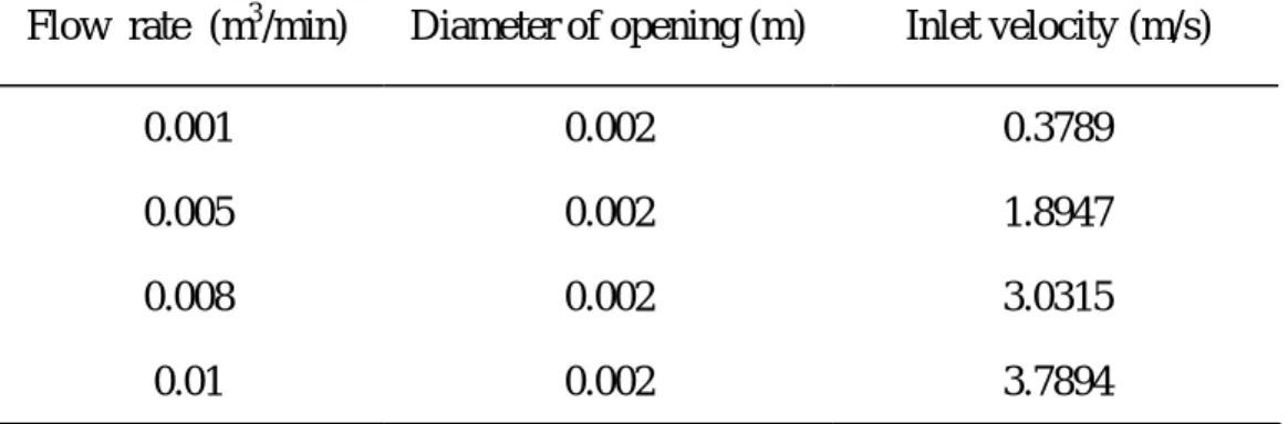
(29) Table 3.1. Information of mass sink. Flow rate (m /min). Diameter of cross section for the sight window(m). Thickness of sink region (m). Fluid removal rate (kg/m3 /s). 4.695. 0.058. 0.003. - 11690.25. 3.13. 0.058. 0.003. - 7793.50. 1.565. 0.058. 0.003. - 3896.75. 0.313. 0.058. 0.003. - 779.35. 3. Table 3.2. Size of calculation domains and grids used for simulation Calculation domain (X * Y * Z). Grids. CPU time (min). 2m * 2m *3m. 393,000. 130. 4m * 4m *5m. 799,000. 280. Table 3.3. Inlet flows at the opening of each gas distribution tube. Flow rate (m3 /min). Diameter of opening (m). Inlet velocity (m/s). 0.001. 0.002. 0.3789. 0.005. 0.002. 1.8947. 0.008. 0.002. 3.0315. 0.01. 0.002. 3.7894. 17.

(30) Fig. 3.1. Sink region at the side window. 18.

(31) (a). (b). 19.

(32) (c). Fig. 3.2. Mesh scheme of the chamber (a) mesh scheme (b) in edge plot (c) in total view.. 20.

(33) (a). (b). Fig. 3.3. Mesh scheme of the chamber with a designed cover (a) mesh scheme (b) in edge plot.. 21.

(34) Chapter 4 Results and discussions 4.1 Simulated airflow field and concentration field (case 1) In the study, the flow and concentration fields were simulated for both case 1 (without the enclosed hood, the chamber is open at the top), and case 2 (with the enclosed hood). Different SF6 release flow rates (1, 5, 8 and 10 L/min) and side venting flow rates (0, 31.3, 93.9, 156.5, 313, 1565, 3130 and 4695 L/min) were simulated. Only the flow and concentration fields of the maximum SF6 flow rate are shown here. Small velocity vectors are difficult to display clearly in the figures, so the following airflow fields are presented using a fixed velocity scale. Fig. 4.1 shows the airflow field when SF6 is released at the flow rate of 10 L/min, and the side venting flow rate is at the maximum of 3130 L/min, at two different cross-section planes of the domain 2x2x3m. Upward injected SF6 flow at the opening of the gas distribution tubes can be observed vividly at the bottom of the chamber. Both airflows inside the chamber and near the chamber top are seen to be sucked into the side window completely. There is no outward SF6 flow at the top of the chamber. The concentration fields of SF6 at the SF6 release flow rate of 10 L/min, and the side venting flow rate of 3130 L/min (100%) is shown in Fig. 4.2. It is observed that with large venting flow rate of 3130 L/min, the SF6 concentration near the top of the chamber is about zero, meaning there is no observable SF6 outflow from the chamber. The results are consistent with the flow fields seen in Fig. 4.1.. 4.2 Comparison between experimental data and simulation results (case 1) To validate the simulation model, the experimental data are compared with the numerical results. Good agreement is obtained. Table 4.1 is the summary of the experimental data for case 1 and case 2, when the side venting flow rate is 3130 L/min. As listed in Table 4.1, the control efficiency by side venting without the hood (case 1) is 95.5%, 97.8%, 98.3%, and 22.

(35) 98.0% for the SF6 release flow rate of 1, 5, 8, and 10 L/min, respectively. The agreement between experimental data and simulation results is greatly affected by the reliability of the boundary conditions used in the calculations. In the simulation, a uniform downward airflow of 0.3 m/s is assigned as one of the inlets at the top boundary of the domain. Table 4.2 shows the simulated control efficiency when the side venting flow rate is 3130 L/min for case 1. Convection is mainly responsible for the control efficiency at different SF6 release flow rates. In smaller domain, the simulated control efficiency are 98.8%, 95.6%, 95.5% and 95.5% at the inlet flow rate of 1, 5, 8, and 10 L/min, respectively. In larger domain, the simulated control efficiency are 99.5%, 96%, 95.4% and 95.7% at the inlet flow rate of 1, 5, 8, and 10 L/min, respectively. The contribution to the control efficiency by diffusion is weak, which is about 0.1%. As shown in Fig. 4.3, the simulation results compare well with the experimental data. Hence, the modeling method and the setting of boundary conditions should be reliable in this study. It is necessary to look into the personnel exposure at the breathing zone after utilizing the side venting method for fully open chamber (case 1). As shown in Fig 4.4, there is no observable SF6 concentration at the breathing zone at different planes when SF6 is released at the flow rate of 10 L/min, and the venting flow rate is at a maximum of 3130 L/min. In Table 4.1, the experimental results of case 1 show that SF6 concentration at the breathing zone is lower than FTIR detection limit of 5 ppb at different SF6 release flow rates. Simulated SF6 concentration at the breathing zone is also lower than FTIR detection limit at different SF6 release flow rates when the side venting flow rate is 3130 L/min, as listed in Table 4.3.. 4.3 Simulated airflow field and concentration field (case 2) In order to simplify the geometrical configuration in the simulation, a cover was designed and installed at the chamber top to simulate the chamber with the enclosed hood (case 2). To. 23.

(36) simulate the wiping of the chamber wall during preventive maintenance, in case 2 the mesh of fluid inside the chamber was assigned to the rotating frame to make the fluid rotating at an angular velocity of 5 rpm about a prescribed axis. Fig. 4.5 shows the airflow field for the chamber with the enclosed hood (case 2) when SF6 is released at the flow rate of 10 L/min, and the venting flow rate is at a maximum of 3130 L/min. It can be observed that downward airflow enters the chamber through the opening of the hood and upward airflow inside the chamber is confined by the hood. Both airflows inside the chamber and near the chamber top are seen to be sucked into the side window more completely. And there is no outward SF6 flow at the opening of the hood. A large circulation exists at the cross plane of the side window by the effect of the rotational fluid inside the chamber. The concentration fields of SF6 at the SF6 release flow rate of 10 L/min, and the venting flow rate of 3130 L/min (100%) is shown in Fig. 4.6, for case2. In Fig. 4.6, it is observed that when there is an enclosed hood at the top of the chamber with the venting flow rate of 3130 L/min, the SF6 concentration near the opening of the hood is about zero, meaning there is no observable SF6 outflow through the opening of the hood then leaving from the chamber.. 4.4 Comparison between experimental data and simulation results (case 2) The measurements and the simulated control efficiency of SF6 versus total gas flow rate when the side venting flow rate is 3130 L/min is shown in Fig. 4.7, for case 2. When the venting flow rate is 3130 L/min, the simulated control efficiency is 100% at the SF6 release flow rate of 1, 5, 8, and 10 L/min. The measurements control efficiency is 97.5% or 98.8% when the SF6 release flow rate is 5 L/min, as listed in Table 4.1. Based on the simulation results, the downward airflow patterns and the enclose hood that confine pollutant to stay in the chamber in combination with the side venting method can enhance the control efficiency. For the chamber with the hood (case 2), in the experimental results SF6 concentration at the 24.

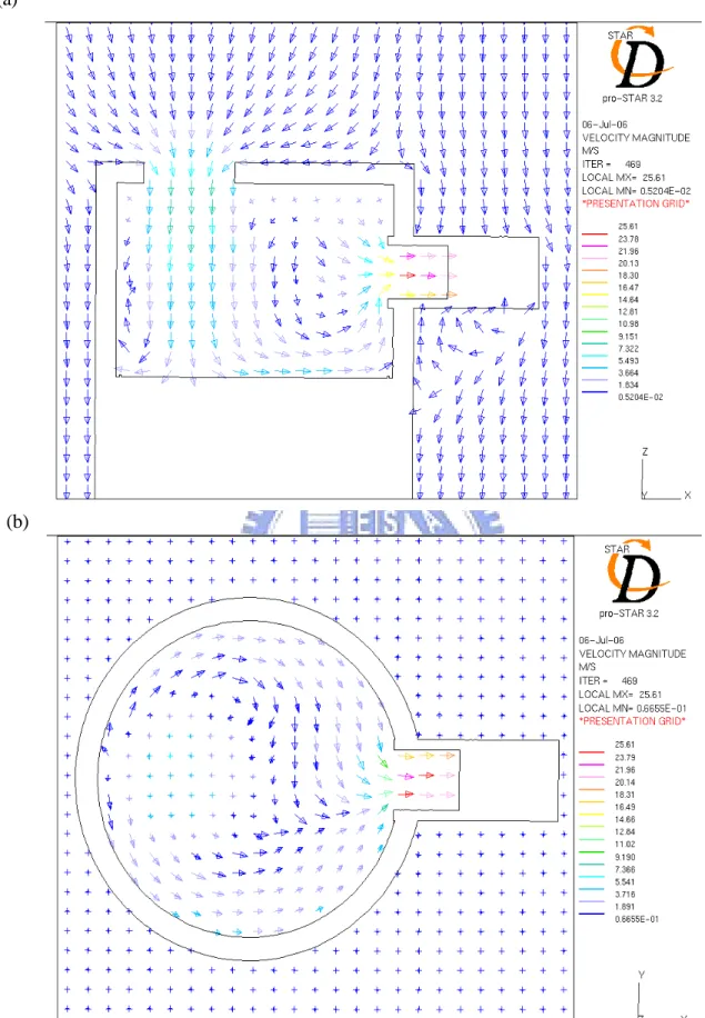
(37) breathing zone is lower than FTIR detection limit (< 5 ppb) when the SF6 release flow rate is 5 L/min and the venting flow rate is 3130 L/min, as listed in Table 4.1. Furthermore, simulated SF6 concentration at the breathing zone is also lower than FTIR detection limit at different SF6 release flow rates when the venting flow rate is 3130 L/min.. 4.5 Simulated airflow field and concentration field at different venting flow rates (case 1) When the venting flow rate is reduced to 10% of the maximum value (or 313 L/min), the flow filed is changed completely, as shown in Fig 4.8. The flow near the side window is still converged into it while some of the flows at the far end of the side window escape the chamber top, leading to potential SF6 leaking into the clean room from the chamber. The concentration fields of SF6 at the SF6 release flow rate of 10 L/min, and the side venting flow rate of 313 L/min (10%) is shown in Fig. 4.9, for case2. In comparison, when the venting flow is small at 313 L/min, significant SF6 concentration exists at the top of the chamber, indicating the leaking of SF6 from the chamber into the clean room. These results are consistent with the flow fields seen in Fig. 4.8. Therefore, to prevent the contamination of the clean room during preventive maintenance, enough venting flow at the side window is effective even when the chamber is open at the top (case 1). When the venting flow rate is too small to capture the air flow effectively, it is quite possible that the contaminant escapes the chamber and pollutes the clean room and the working personnel. When the venting flow rate is zero, the flow fields for case 1 is shown in Fig. 4.10. It is observed that the downward clean room air flow enters the chamber, mixes with the SF6 release flow and then leaves at the top of the chamber. The SF6 concentration field in Fig. 4.11 further shows that SF6 leaves from the top of the chamber into the clean room creating pollution of the room. Therefore, without the venting flow, contamination of the clean room is serious. Although the pollutant concentration is possible low at the breathing zone after 25.

(38) dispersion, contamination still pose health risks to workers and causes wafer defects and process tool corrosion due to the air recirculation and change in the clean room. The occupational hygiene of these workers and the problem how to apply the side venting method properly deserve attentions.. 4.6 Simulation results at different venting flow rates (case 1) The control efficiencies of side venting at different flow rates were investigated by changing the mass flow rate of sink in the simulation. Table 4.4 shows the simulated control efficiency when the side venting flow rate is 313 L/min for case 1. In smaller domain, the control efficiency are 81.9%, 72.7%, 74.7% and 73.5% at the inlet flow rate of 1, 5, 8, and 10 L/min, respectively. In larger domain, the control efficiency are 85.4%, 75.2%, 76.3% and 76.5% at the inlet flow rate of 1, 5, 8, and 10 L/min, respectively. These results are consistent with the flow and concentration fields seen in Fig. 4.8 and Fig. 4.9 that SF6 concentration exists at the top of the chamber when the side venting flow rate is reduced to 313 L/min. Although a very small concentration is increased when the side venting flow rate is reduced to 313 L/min, simulated SF6 concentration at the breathing zone is also lower than FTIR detection limit whether the venting flow rate is 3130 L/min or 313 L/min, as listed in Table 4.3. The side venting method is effective to control pollutant dispersion and improve the air quality in the clean room. The simulated control efficienc y of SF6 versus total gas flow rate when the side venting flow rate is reduced to 50%, 10%, 5%, 3%, or 1% of the maximum value (1565 L/min, 313 L/min, 156.5 L/min, 93.9 L/min, or 31.3 L/min) are shown in Fig. 4.12, Fig. 4.13, Fig. 4.14, Fig. 4.15, and Fig. 4.16, respectively. In Fig. 4.12, the simulated control efficiency is still above 95% when the side venting flow rate is reduced to 50% (or 1565 L/min). However, the simulated control efficiency keeps in low va lues at different SF6 release flow rates when the. 26.

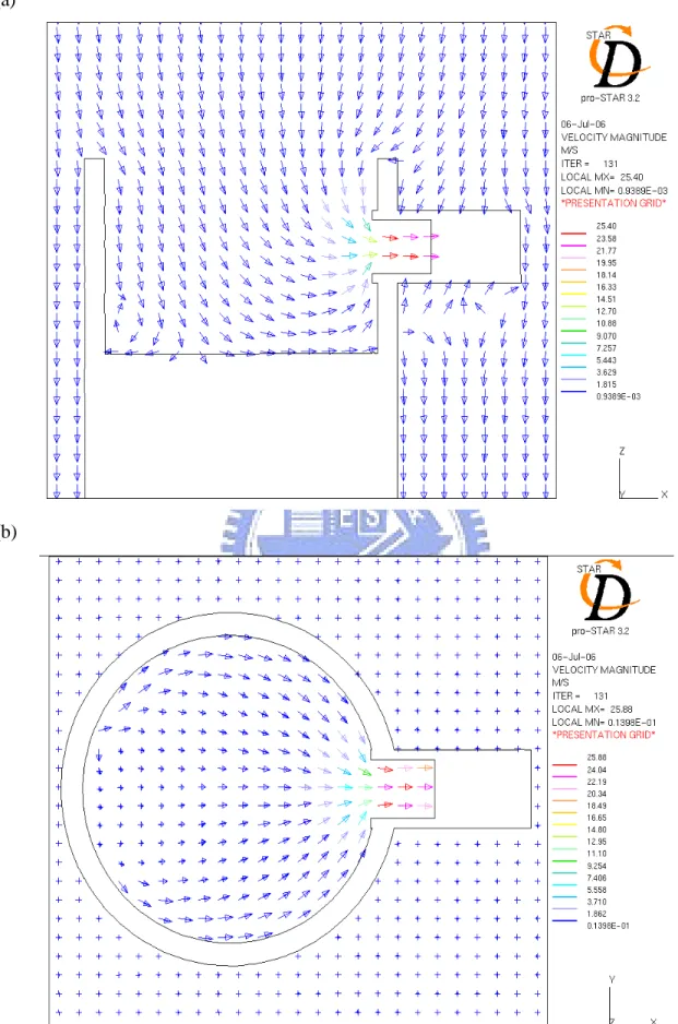
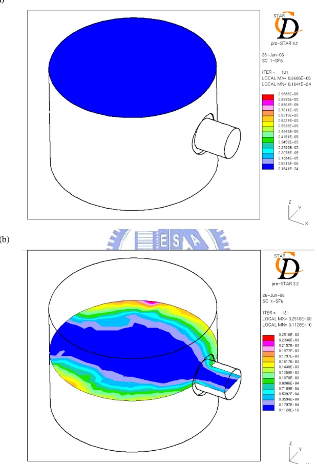
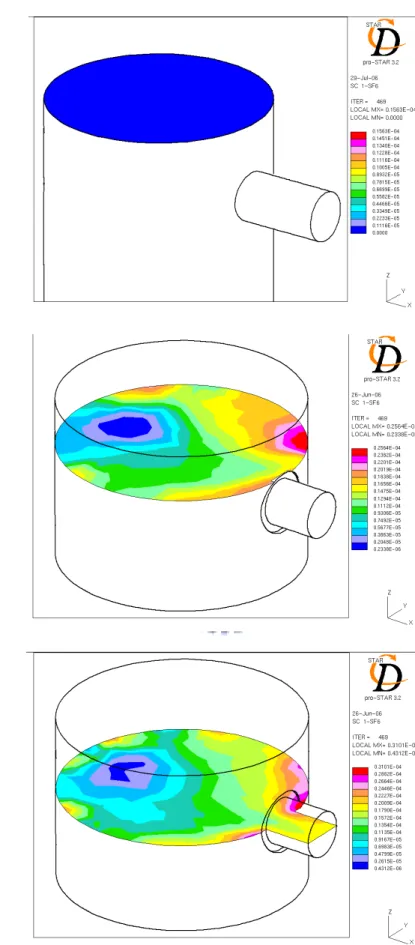
(39) side venting flow rate is reduced to 1% (or 31.3 L/min), as shown in Fig. 4.16. In Fig. 4.17, the control efficiency increases very close to 100% with the increasing of the side venting flow rate to 150% of the maximum value (or 4950 L/min). Simulated control efficiency of SF6 versus different side venting flow rates when SF6 release flow rate is 10 L/min, 8 L/min, 5L/min, and 1L/min are shown in Fig. 4.18, Fig. 4.19, Fig. 4.20, and Fig. 4.21, respectively. Although there are many parameters and operation conditions that could influence the control efficiency of the chamber without the hood by side venting, this study has found that the side venting flow rate is the most important parameter. For example, for the simulated control efficiency of SF6 shown in Fig. 4.18, when the side venting flow rate is less than about 700 L/min, the control efficiency increases with the increasing venting flow rate. When the side venting flow rate is higher than 1200 L/min, the control efficiency is found to be higher nearly 100% and becomes more or less a constant. Similar trend also occurs for SF6 release flow rate is 8 L/min, 5L/min, and 1L/min. For case 1, the results show that side venting at a large flow rate should be an effective way to control pollutant dispersion and reduce the worker’s exposure during preventive maintenance.. 4.7 Simulation results at different venting flow rates (case 2) When the venting flow rate is reduced to 10% of the maximum value (or 313 L/min), the flow filed is similar to the results of the venting flow rate of 3130 L/min for the chamber with the hood, as shown in Fig 4.22. The flow near the side window is still converged into it. A large circulation exists at the cross plane of the side window by the effect of the rotational fluid inside the chamber. The concentration fields of SF6 at the SF6 release flow rate of 10 L/min, and the venting flow rate of 313 L/min (10%) is shown in Fig. 4.23, for case2. In comparison with the venting flow rate of 3130 L/min, it is also observed that when there is an enclosed hood at the top of the chamber with the venting flow rate of 313 L/min, the SF6. 27.

(40) concentration near the opening of the hood is about zero, meaning there is also no observable SF6 outflow through the opening of the hood then leaving from the chamber. As shown in Fig. 4.24, when the venting flow rate is 313 L/min, the simulated control efficiency for case2 is 100% at the SF6 release flow rate of 1, 5, 8, and 10 L/min. When the venting flow rate is zero, the flow and SF6 concentration fields for case 2 are shown in Fig. 4.25 and Fig. 4.26, respectively. In Fig. 4.25, it can be seen that without side venting the downward clean room air flow enters the chamber through the opening of the hood, then also mixes with the SF6 release flow and leaves from the opening of the hood. The SF6 concentration field in Fig. 4.26 further shows that SF6 can leaves from the opening of the hood and the rest of SF6 concentration accumulate at the lower side of the hood. Dispersion of SF6 is restricted to the downward airflow and the installation of the hood. It can be concluded that high degree isolation can effectively protect the worker’s exposure by the effect of installing the hood in combination with the side venting method at a large flow rate during preventive maintenance.. 28.

(41) Table 4.1. Experimental data under different conditions when the side venting flow rate is 3130 L/min (Ku, 2004).. Control SF6 flow rate SF6 Concentration at SF6 concentrationa SF6 concentrationb Case breathing zone (ppm) efficiency (%) (ppm) (ppm) (L/min) 5. 2. N.D.. 0.78. 0.80. 97.5. 5. 2. N.D.. 0.81. 0.82. 98.8. 1. 1. N.D.. 0.21. 0.22. 95.5. 5. 1. N.D.. 0.88. 0.90. 97.8. 8. 1. N.D.. 1.18. 1.20. 98.3. 10. 1. N.D.. 1.46. 1.49. 98.0. a : SF6 concentration at the end point of the low vacuum venting line when SF6 is released at the bottom of the chamber. b : SF6 concentration at the end point of the low vacuum venting line when SF6 is released inside the low vacuum line. Table 4.2. Simulated control efficiency when the side venting flow rate is 3130 L/min, case 1. Experimental Calculation domain Flow rate control efficiency (X*Y*Z) (L/min) (%) 2m*2m*3m. 4m*4m*5m. Control efficiency (%). Contribution by Contribution by convection (%) diffusion (%). 1. 95.5. 98.8. 98.68. 0.12. 5. 97.8. 95.6. 95.52. 0.11. 8. 98.3. 95.5. 95.42. 0.11. 10. 98.0. 95.5. 95.43. 0.12. 1. 95.5. 99.5. 99.36. 0.17. 5. 97.8. 96.0. 95.84. 0.16. 8. 98.3. 95.4. 95.25. 0.16. 10. 98.0. 95.7. 95.55. 0.16. 29.

(42) Table 4.3. Simulated SF6 concentration at the breathing zone when the side venting flow rate is 3130 L/min or 313 L/min, case1.. SF6 concentration at the breathing zone, side venting flow rate of 3130 L/min (ppb). SF6 concentration at the breathing zone, side venting flow rate of 313 L/min (ppb). 1. 7.70 x 10-28. 3.18 x 10-8. 5. 2.07 x 10-28. 3.69 x 10-8. 8. 6.56 x 10-25. 1.21 x 10-8. 10. 1.01 x 10-24. 3.99 x 10-8. 1. 1.47 x 10-26. 1.88 x 10-14. 5. 1.50 x 10-22. 2.6 x 10-12. 8. 1.85 x 10-22. 4.47 x 10-13. 10. 2.33 x 10-22. 4.84 x 10-12. Calculation domain Flow rate (X*Y*Z) (L/min) 2m*2m*3m. 4m*4m*5m. Table 4.4. Simulated control efficiency when the side venting flow rate is 313 L/min, case 1 Calculation domain Flow rate (X*Y*Z) (L/min) 2m*2m*3m. 4m*4m*5m. Control efficiency (%). Contribution by Contribution by convection (%) diffusion (%). 1. 81.9. 80.37. 1.53. 5. 72.7. 71.67. 1.06. 8. 74.7. 73.9. 0.74. 10. 73.5. 72.7. 0.80. 1. 85.4. 83.10. 2.37. 5. 75.2. 73.68. 1.57. 8. 76.3. 75.21. 1.13. 10. 76.5. 75.72. 0.84. 30.

(43) (a). (b). Fig. 4.1. Velocity vector for SF6 release flow rate of 10 L/min, venting flow rate of 3130 L/min in the 2x2x3m domain, case 1 (a) xz plane (b) xy plane. 31.

(44) (a). (b). Fig. 4.2. Concentration distribution for SF6 release flow rate of 10 L/min, venting flow rate of 3130 L/min in the 2x2x3m domain, case 1 (a) plane across the chamber top (b) plane across the side window.. 32.

(45) Control Efficiency (%). 100. 80. SF6 Control Efficiency SF 6=1000ppm (exp. results) SF 6=1000ppm (sim. results, domain 2x2x3) SF 6=1000ppm (sim. results, domain 4x4x5). 60. 40. 20. 0 0. 2. 4 6 QSF (L/min). 8. 10. 6. Fig. 4.3. Measurements and simulated control efficiency of SF6 versus total gas flow rate when the side venting flow rate is 3130 L/min, case 1.. 33.

(46) (a). (b). Fig. 4.4. Concentration distribution at the breathing zone for SF6 release flow rate of 10 L/min, venting flow rate of 3130 L/min in the 2x2x3m domain, case 1 (a) xz plane (b) the plane across the center of domain. 34.

(47) (a). (b). Fig. 4.5. Velocity vector of the chamber with the hood for SF6 release flow rate of 10 L/min, venting flow rate of 3130 L/min in the 2x2x3m domain, case 2 (a) xz plane (b) xy plane. 35.

(48) (a). (b). (c). Fig. 4.6. Concentration distribution of the chamber with the hood for SF6 release flow rate of 10 L/min, venting flow rate of 3130 L/min in the 2x2x3m domain, case 2.. 36.

(49) Control Efficiency (%). 100. 80. SF6 Control Efficiency SF 6=1000ppm (exp. results) SF 6=1000ppm (sim. results, domain 2x2x3) SF 6=1000ppm (sim. results, domain 4x4x5). 60. 40. 20. 0 0. 2. 4 6 QSF (L/min). 8. 10. 6. Fig. 4.7. Measurements and simulated control efficiency of SF6 versus total gas flow rate when the side venting flow rate is 3130 L/min, case 2.. 37.


(51) (a). (b). Fig. 4.9. Concentration distribution for SF6 release flow rate of 10 L/min, venting flow rate of 313 L/min in the 2x2x3m domain, case 1 (a) plane across the chamber top (b) plane across the side window. 39.


(53) (a). (b). Fig. 4.11. Concentration distribution for SF6 release flow rate of 10 L/min, venting flow rate of 0 L/min in the 2x2x3m domain, case 1 (a) plane across the chamber top (b) plane across the side window.. 41.

(54) Control Efficiency (%). 100. 80. 60 SF6 Control Efficiency. 40 SF 6=1000ppm (sim. results, domain 2x2x3) SF 6=1000ppm (sim. results, domain 4x4x5). 20. 0 0. 2. 4 6 QSF (L/min). 8. 10. 6. Fig. 4.12. Simulated control efficiency of SF6 versus total gas flow rate when the side venting flow rate is 1565 L/min, case 1.. 42.

(55) Control Efficiency (%). 100. 80. 60 SF6 Control Efficiency. 40 SF 6=1000ppm (sim. results, domain 2x2x3) SF 6=1000ppm (sim. results, domain 4x4x5). 20. 0 0. 2. 4 6 QSF (L/min). 8. 10. 6. Fig. 4.13. Simulated control efficiency of SF6 versus total gas flow rate when the side venting flow rate is 313 L/min, case 1.. 43.

(56) Control Efficiency (%). 100. 80. 60. 40 SF6 Control Efficiency. 20. SF6=1000ppm (sim. results, domain 2x2x3) SF6=1000ppm (sim. results, domain 4x4x5). 0 0. 2. 4 6 QSF (L/min). 8. 10. 6. Fig. 4.14. Simulated control efficiency of SF6 versus total gas flow rate when the side venting flow rate is 156.5 L/min, case 1.. 44.

(57) 100. Control Efficiency (%). SF6 Control Efficiency. 80. SF6=1000ppm (sim. results, domain 2x2x3) SF6=1000ppm (sim. results, domain 4x4x5). 60. 40. 20. 0 0. 2. 4 6 QSF (L/min). 8. 10. 6. Fig. 4.15. Simulated control efficiency of SF6 versus total gas flow rate when the side venting flow rate is 93.9 L/min, case 1.. 45.

(58) Control Efficiency (%). 100. 80 SF6 Control Efficiency. 60. SF6=1000ppm (sim. results, domain 2x2x3) SF6=1000ppm (sim. results, domain 4x4x5). 40. 20. 0 0. 2. 4 6 QSF (L/min). 8. 10. 6. Fig. 4.16. Simulated control efficiency of SF6 versus total gas flow rate when the side venting flow rate is 31.3 L/min, case 1.. 46.

(59) Control Efficiency (%). 100. 80. 60 SF6 Control Efficiency. 40 SF 6=1000ppm (sim. results, domain 2x2x3) SF 6=1000ppm (sim. results, domain 4x4x5). 20. 0 0. 2. 4 6 QSF (L/min). 8. 10. 6. Fig. 4.17. Simulated control efficiency of SF6 versus total gas flow rate when the side venting flow rate is 4695 L/min, case1.. 47.

(60) Control Efficiency (%). 100. 80. 60 SF6 Control Efficiency. 40 SF6=1000ppm (sim. results, domain 2x2x3) SF6=1000ppm (sim. results, domain 4x4x5). 20. 0 0. 1000. 2000 3000 Qventing (L/min). 4000. 5000. Fig. 4.18. Simulated control efficiency of SF6 versus different side venting flow rates when SF6 release flow rate is 10 L/min, case1.. 48.





(65) (a). (b). (c). Fig. 4.23. Concentration distribution of the chamber with the hood for SF6 release flow rate of 10 L/min, venting flow rate of 313 L/min in the 2x2x3m domain, case 2.. 53.

(66) Control Efficiency (%). 100. 80. SF6 Control Efficiency SF 6=1000ppm (sim. results, domain 2x2x3) SF 6=1000ppm (sim. results, domain 4x4x5). 60. 40. 20. 0 0. 2. 4 6 QSF (L/min). 8. 10. 6. Fig. 4.24. Simulated control efficiency of SF6 versus total gas flow rate when the side venting flow rate is 313 L/min, case 2.. 54.


(68) (a). (b). (c). Fig. 4.26. Concentration distribution of the chamber with the hood for SF6 release flow rate of 10 L/min, venting flow rate of 0 L/min in the 2x2x3m domain, case 2. 56.

(69) Chapter 5 Conclusions This study presents the numerical simulation results which were verified with the experimental data to evaluate the control efficiency of the chamber with the hood at the chamber top, or witho ut the hood by side venting at the large flow rate during preventive maintenance. The control efficiency of side venting at different flow rates was also investigated. The airflow and concentration fields were calculated numerically. Results show that pollutant dispersion of a metal dry etcher during preventive ma intenance can be effectively controlled by side venting at a large flow rate near the chamber top whether the chamber is fully open (without the hood) or with the hood. Good agreement between the experimental data and the simulation results is obtained. The SF6 concentration at the breathing zone was also found to be lower than the detection limit of the FTIR. When the side venting flow rate is reduced but maintaining above a fixed value, the pollutant dispersion still can be effectively controlled, and the control efficiency of the chamber with the hood is superior to that of the chamber without the hood. The results also indicate that computational fluid dynamics simulation has potential for modeling local ventilation systems of a metal etcher during preventive maintenance in the clean room. It is a useful tool to design more efficient local contaminant control systems in semiconductor industry and for metal etching equipments manufacturer based on the understanding of the proposed control method. However, the verification of numerical modeling under controlled conditions is necessary. The reliability of the boundary conditions used in the calculations needs careful test. The numerical simulations are restricted to the conditions where the worker ’s cleaning actions is absent. Further research is requir ed to accurately consider the influence of worker ’s cleaning actions during preventive maintenance on the control efficiency of the hood. SF6 concentration variations with time during preventive maintenance also have not been determined by numerical simulations. 57.

(70) Reference Bauer, S., Werner, N., Wolff, I., Damme, B., Oemus, K., Hoffmann, P. (1992) Toxicological Investigation in the Semiconductor Industry: II Studies on the Subacute Inhalation Toxicity and Genotoxicity of Gaseous Waste Products from the Aluminium Plasma Etching Process, Toxicology and Industrial Health, 8(6), 431-444. Bauer, S., Wolff, I., Werner, N., Schmidt, R., Blume, R., Pelzing, M. (1995) Toxicological Investigation in the Semiconductor Industry: IV Studies on the Subchronic Oral Toxicity and Genotoxicity of Vacuum Pump Oil Contaminated by Waste Products from Aluminium Plasma Etching Processes, Toxicology and Industrial Health, 11(5), 523-541. Bauer, S., Wolff, I., Schmidt, R., Pelzing, M. (1996) Toxicological Hazards of Plasma Etching Waste Products, Solid State Technology, 39(7), 97-110. Chang, C. P., Song, L. Y., Chu, C. Q., Lin, Y. C. (2000) The Evaluation of Hazardous Gases Emission from the Preventive Maintenance Procedure in Semiconductor Factory, IOSH(Taiwan) Quarterly, 8(2), 205-216. Cussler, E. L. (1997) Diffusion Mass Transfer in Fluid Systems, 2nd Ed ition, Cambridge University Press, Cambridge Hampl, V. (1984) Evaluation of Industrial Exhaust Hood Efficiency by a Tracer Gas Technique, American Industrial Hygiene Association Journal, 45(7), 485-490. Hampl, V., Niemela, R., Shulman, S., Bartley, D. L. (1986) Use of Tracer for Industrial Exhaust Hood Efficiency Evaluation – Where to Sample, American Industrial Hygiene Association Journal, 47(5), 281-287. Heinonen, K., Kulmala, I., Saamamen, A. (1996) Local Ventilation for Powder Hand ling Combination of Local Supply and Exhaust Air, American Industrial Hygiene Association Journal, 57(4), 356-364.. 58.

(71) Ivany, R. E., First, M. W., Diberardinis, L. J. (1989) A New Method for Quantitative, In-Use Testing of Laboratory Fume Hoods, American Industrial Hygiene Association Journal, 50(5), 275-280. Kulmala, I. (1994) Numerical Simulation of a Local Ventilation Unit, Annals of Occupational Hygiene, 38(4), 337-349. Kulmala, I. (1995) Numerical Simulation of the Capture Efficiency of an Unflanged Rectangular Exhaust Opening in a Coaxial Airflow, Annals of Occupational Hygiene, 39(1), 21-33. Kulmala, I. (1995) Numerical Simulation of an Unflanged Rectangular Exhaust Openings, American Industrial Hygiene Association Journal, 56(11), 1099-1106. Kulmala, I., Saarenrinne, P. (1996) Air Flow near an Unflanged Rectangular Exhaust Opening, Energy and Buildings, 24(2), 133-136. Kulmala, I. (2000) Experimental Validation of Potential and Turbulent Flow Models for a Two-dimensional Jet Enhanced Exhaust Hood, American Industrial Hygiene Association Journal, 61(2), 183-191. Ku, K. W. (2004) Controlling Pollutant Dispersion during Preventative Maintenance of a Metal Etcher in Semiconductor Factory, National Chiao Tung University, Master Thesis, Taiwan Li, S. N., Chang, C. T., Shin, H. Y., Tang, A., Li, A., Chen, Y.Y. (2003) Using an Extractive Fourier Transform Infrared Spectrometer for Improving Cleanroom Air Quality in a Semiconductor Manufacturing Plant, American Industrial Hygiene Association Journal, 64(3), 408-414. Li, S. N., Shin, H. Y., Wang, K. S., Hsieh, K., Chen, Y.Y., Chen, Y.Y., Chou, J. (2005) Preventive Maintenance Measures for Contamination Control, Solid State Technology, 48(12), 53-56.. 59.

(72) Muller, P., Stock, T., Bauer, S., Wolff, I. (2002) Genotoxicological Characterisation of Complex Mixtures Genotoxic Effects of a Complex Mixture of Perhalogenated Hydrocarbons, Mutation Research Genetic Toxicology and Environmental Mutagenesis, 515(1-2), 99-109. Patankar, S.V., Spalding, D. B. (1972) A Calculation Procedure for Heat, Mass and Momentum Transfer in Three-dimensional Parabolic Flows, Intternational Journal of Heat and Mass Transfer, 15, 1787-1806. Schmidt, R., Scheufler, H., Bauer, S. Wolff, L., Pelzing, M., Herzschuh, R. (1995) Toxicological Investigation in the Semiconductor Industry: III Studies on Prenatal Toxicity Caused by Waste Products from Aluminum Plasma Etching Processes, Toxicology and Industrial Health, 11(1), 49-61. STAR-CD Version 3.22 Methodology (2004) Computational Dynamic limited.. 60.

(73) Appendix fluinj.f C************************************************************************* SUBROUTINE FLUINJ(FLUXI,UI,VI,WI,TEI,EDI,TI,SCINJ,IPMASS) C Fluid injection C************************************************************************* C--------------------------------------------------------------------------* C STAR VERSION 3.20.000 * C--------------------------------------------------------------------------* INCLUDE 'comdb.inc' DIMENSION SCINJ(50) COMMON/USR001/INTFLG(100) INCLUDE 'usrdat.inc' DIMENSION SCALAR(50) EQUIVALENCE( UDAT12(001), ICTID ) EQUIVALENCE( UDAT03(001), CON ) EQUIVALENCE( UDAT03(019), VOLP ) EQUIVALENCE( UDAT04(001), CP ) EQUIVALENCE( UDAT04(002), DEN ) EQUIVALENCE( UDAT04(003), ED ) EQUIVALENCE( UDAT04(005), PR ) EQUIVALENCE( UDAT04(008), TE ) EQUIVALENCE( UDAT04(009), SCALAR(01) ) EQUIVALENCE( UDAT04(059), U ) EQUIVALENCE( UDAT04(060), V ) EQUIVALENCE( UDAT04(061), W ) EQUIVALENCE( UDAT04(062), VISM ) EQUIVALENCE( UDAT04(063), VIST ) EQUIVALENCE( UDAT04(007), T ) EQUIVALENCE( UDAT04(067), X ) EQUIVALENCE( UDAT04(068), Y ) EQUIVALENCE( UDAT04(069), Z ) C------------------------------------------------------------------------C C This subroutine enables the user to specify fluid injection C (addition or removal) into live cells. In the case of mass C removal (sink), only the mass flux (FLUXI) can be specified. In 61.

(74) C the case of mass addition (source), the fluid will bring all its C user-specified properties (momentum, turbulence, temperature and C concentrations). Zero will be assumed for omitted properties. C C ** Parameters to be returned to STAR: C (Sink) FLUXI (<0) C (Source) FLUXI (>0),UI,VI,WI,TEI,EDI,TI,SCINJ,IPMASS C C IPMASS is an interphase mass transfer indicator used in C Eulerian two-phase (E2P) simulations only. C The default value, passed from STAR to FLUINJ, is always zero. C IPMASS=0: no interphase heat transfer - the mass sources specified C in FLUINJ are independent for each phase. C IPMASS=1: the phases are exchanging mass - the mass source specified C is directed from one phase into the other phase. C For more information, please refer to the E2P sections of the C manuals. C C------------------------------------------------------------------------C C Sample coding: Fluid injection and removal C C IF(ICTID.EQ.3) THEN CC Injection C FLUXI=0.1 C WI=0.05 C TI=373.0 C SCINJ(1)=1.0 C ELSE IF(ICTID.EQ.4) THEN CC Removal IF(ICTID.EQ.9) THEN FLUXI=-7793.5 ENDIF C-------------------------------------------------------------------------C RETURN END C. 62.

(75)