國 立 交 通 大 學
材料科學與工程學系
奈米科技碩博士班
碩 士 論 文
氮化矽微米孔隙元件於細胞濃度快速鑑別研究
Rapid resolving of bead and cell concentrations by
silicon nitride micropore sieve device
研 究 生:徐筱淋 (Hsiao-Lin Hsu)
指導教授:許鉦宗 教授 (Prof. Jeng-Tzong Sheu)
氮化矽微米孔隙元件於細胞濃度快速鑑別研究
Rapid resolving of bead and cell concentrations by
silicon nitride micropore sieve device
研究生:徐筱淋 Student:Hsiao-Lin Hsu
指導教授:許鉦宗 教授 Advisor:Prof. Jeng-Tzong Sheu
國立交通大學
材料科學與工程學系奈米科技碩博士班
碩士論文
A thesis
Submitted to Graduate Program for Nanotechnology
Department of Materials Science and Engineering,
National Chiao Tung University
in partial Fulfillment of the Requirements
for the Degree of Master
in
Institute of Nanotechnology
July, 2013
Hsinchu 300, Taiwan
I
Rapid resolving of bead and cell concentrations by
silicon nitride micropore sieve device
Student:
Hsiao-Lin Hsu
Advisor: Dr. Jeng-Tzong SheuInstitute of Nanotechnology, Department of Materials Science and Engineering
National Chiao Tung University
Abstract
In this research, silicon nitride micropore sieve was prepared and applied to resolve bead and cell concentrations via the measurement of the conductance across the pore. The micropore sieve was fabricated via microfabrication processes on the free standing silicon nitride membrane with the pore number ranging from 9 to 484. Electrical equivalent circuit model of the micropore sieve device was constructed and compared with the measurement data. Analytes were flowed through the micropores at a flow rate of 20 µl min-1 via a syringe pump. The AC sine-wave voltage (10 mV rms) at 10 Hz was applied between two Ag/AgCl electrodes across the micropores by a lock-in amplifier, and the ionic current was analyzed. Polystyrene beads and HeLa cells concentrations were characterized separately. Devices with different pore number were optimized and applied to resolve the beads/HeLa cells concentration. In 2 minutes, the device with 49 micropores exhibited the best resolving ability for polystyrene bead and HeLa cells concentration ranging from 102/ml to 106/ml.
II
氮化矽微米孔隙元件於細胞濃度快速鑑別研究
研究生:徐筱淋 指導教授:許鉦宗 教授
國立交通大學
材料科學與工程學系奈米科技碩士班
摘 要
本研究利用微米孔洞陣列氮化矽薄膜作為細胞濃度偵測之元件。
量測通過微米孔洞的導電度以分析檢體中粒子的濃度。首先,利用微
米製作技術製備出氮化矽微米孔洞陣列薄膜,孔洞數分別為 9、49、
100、484。經由電路模型的建立分析以及實際量測結果,決定後續實
驗中施加電壓的操作頻率。實驗過程中,檢體以固定流速,20 µl/min
的流速進入流道中,電壓由鎖相放大器經由氯化銀參考電極供給並且
同時量測電流值變化,操作條件為 10 mV,頻率 10 Hz。本實驗分別
量測了聚苯乙烯粒子以及子宮頸癌細胞的濃度。實驗過程中,以不同
孔洞數量的元件量測檢體中粒子濃度,並且比較其結果。結果顯示,
擁有孔洞數為 49 的元件於兩分鐘可達到最佳的濃度鑑別能力,其對
於聚苯乙烯粒子以及子宮頸癌細胞的濃度鑑別範圍為 10
2/ml to
10
6/ml。另外,在此量測系統中,所需要的量測時間不到兩分鐘,本
研究成功的提出了可以快速量測粒子濃度的系統
。III
致 謝
猶記得兩年前剛踏入實驗室時對於研究這回事懵懵懂懂,經過這段時間的學 習漸漸的培養了獨立研究的能力,這一路走來感謝身邊所有人的支持與教導。首 先感謝我的指導教授,許鉦宗教授,提供了設備完善的研究環境以及獨立思考的 空間,讓我可以無後顧之憂的完成我的研究。另外,感謝口委們提出的建議,讓 我的論文更加完善。感謝陳振嘉博士,總是耐心的和我討論實驗上遇到的困難, 教導我如何系統性的思考與設計實驗,並且與我分享了許多待人處事的方法,對 於人生價值觀與規畫也給了我不一樣的思考方式。 碩士班兩年的實驗室生活沒有當初想像的枯燥可怕,反之,我們實驗室就像 是個溫馨的大家庭一樣,大家總是互相幫忙互相照應。感謝皓恆學長提供我研究 上的建議,教我以樂觀積極的態度去面對困境,並且在我遇到瓶頸時鼓勵我繼續 堅持下去。感謝老翔在我遇到困難時提供協助及建議,感謝志偉在我實驗初期提 供了許多流道架設的建議以及教我許多電性量測的原理,感謝滷蛋和小桑時常和 我討論實驗以及聊天舒壓。感謝俏屁在碩一時的帶領,教會了我許多機台和實驗 技巧並且不厭其煩的固定和我討論 paper 交換想法,感謝華哥時常提醒我處理問 題的方法還與我分享了許多人生大道理。感謝我的好同學 Zoe 和嘉哲,一起修課, 做研究,一起朝著畢業的目標邁進,互相扶持幫忙陪我度過這兩年。感謝芋頭一 直以來提供了我許多量測時用到的細胞。還有許多實驗室的夥伴,東哥、猴子、 珮琳、舒鈺、仲廷、番茄,這兩年,和大家一起討論、聚餐、談心、出遊、運動 都是美好且難忘的回憶。 最後感謝我的家人與朋友,感謝我的父母對我求學的抉擇始終支持,提供我 經濟和精神上充裕的支援,讓我可以無後顧之憂的完成我的學業。感謝我的好友 們無時無刻給我精神支援,當我停下來休息時總給我滿滿的油量繼續向前邁進。 因為有大家的支持與鼓勵才能讓我順利完成學業,繼續往下一個目標邁進。IV
Table of content
Abstract ... I 摘 要 ... II 致 謝 ... III Table of content ... IV List of the figure ... VII List of the table ... XIIChapter 1 Introduction ... 1
1-1 Foreword ... 1
1-2 The application of cell counting ... 2
1-3 Present technology to count cells ... 3
1-4 The applications of micropores ... 9
1-5 The electrical circuit model of micropore ... 11
1-5-1 Pore resistance ... 11
1-5-2 Membrane capacitance ... 12
1-5-3 Electrolyte resistance ... 13
1-6 Motivation ... 14
1-6-1 Motivation ... 14
1-6-2 Goal of this study ... 14
Chapter 2 Device Preparation... 15
2-1 Device fabrication process ... 15
2-1-1 Silicon wafer clean ... 15
2-1-2 Silicon nitride deposition ... 16
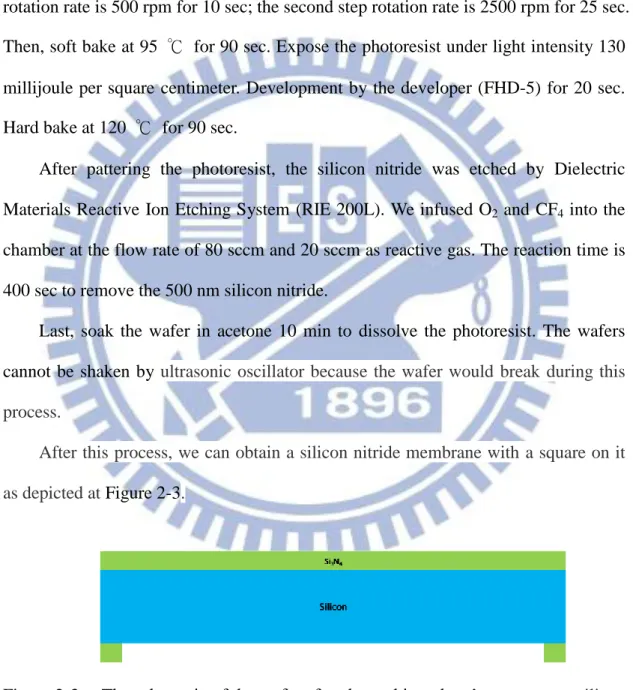
2-1-3 Top side pattern ... 16
V
2-1-5 Wet etching ... 19
2-2 Device analysis ... 20
2-2-1 SEM and OM image ... 20
2-2-2 Membrane thickness analysis ... 20
2-2-3 Pore diameter analysis ... 21
2-3 Cell culture process ... 22
2-4 Polystyrene beads sample preparing process ... 23
2-5 Acrylic block design ... 25
2-6 Microfluidic Fixture ... 26
2-7 Set-up of Measurement equipment... 28
Chapter 3 Equivalent Circuit ... 29
3-1 Theoretic value of pore resistance and device resistance ... 29
3-1-1 Maximum and minimum value of pore resistance ... 29
3-1-2 Device resistance for single pore and multiple pores ... 30
3-2 Massurement of pore resistance and device resistance ... 33
3-2-1 Micro-pores device characteristic analysis ... 33
3-2-2 Micro-pores device with polystyrene beads measurement... 35
3-3 Frequency effect ... 38
3-4 Working Frequency ... 39
Chapter 4 Results and Discussion ... 42
4-1 Current drop caused from polystyrene beads ... 42
4-1-1 49 pores device ... 42
4-1-2 9 pore device experiment ... 42
4-2 Beads measurement results and discussion ... 46
4-2-1 Resolving of bead concentrations ... 46
4-2-2 Discussion ... 52
VI
Chapter 5 Conclusion and future work ... 57
5-1 Conclusion ... 57
5-2 Future work ... 58
VII
List of the figure
Figure 1-1. Schematic of a Hemocytometer. [18] ... 3 Figure 1-2. Schematic of a Coulter counter. [19] ... 5 Figure 1-3. Schematic of a cell separator. [4] ... 5 Figure 1-4. Microfluidic devices and the experimental set up for impedance
spectroscopy measurement. (a) Schematic drawing of the impedance measurement set up. (b) Illustration showing measurement of cell ion release using impedance spectroscopy. (c)–(e) Details of the electrode layout and device. [5] ... 6 Figure 1-5. The schematic of fluorescence-based flow cytometry. [7] ... 7 Figure 1-6. Detail of V-groove and optics. Dashed lines indicate scattered
light due to a red blood cell (RBC). [8] ... 8 Figure 1-7. Sorting results for different sizes of PS particles. (A) Particle
mixture measurement before sorting; (B), (C), and (D) measurement of the smallest, intermediate and largest collected particles, respectively. [12] ... 9 Figure 1-8. Sorting results of whole blood. (A) Particle distribution
measurements of whole blood before sorting; (B) particle distribution measurements of collected red blood cells and platelets; and (C)
collected white blood cells and REH cells. [12] ... 10 Figure 1-9. The schematic model of the circuit. ... 11 Figure 1-10. Total channel resistance is a sum of the resistance of the
channel proper and access resistances at both sides of the channel.[17] ... 12 Figure 1-11. Schematics of the lumped element models superimposed on the physical geometry (not to scale) of a nitride membrane. [14] ... 13 Figure 2-1. The schematic of a silicon wafer with 500 nm silicon nitride
membrane at both side. ... 16 Figure 2-2. The top side mask pattern. ... 16 Figure 2-3. The schematic of the wafer after dry etching, there’s a square
on silicon nitride membrane... 17 Figure 2-4. The bottom side mask pattern. ... 18 Figure 2-5. Design of different pore numbers on the mask. ... 18 Figure 2-6. The schematic of silicon nitride membrane with micropore
VIII
Figure 2-7. The schematic of the micro-pores sieve. ... 19
Figure 2-8. The optical microscope and scanning electron microscope image of the device. Scale bar: 10 m. ... 20
Figure 2-9. The positions of silicon nitride thickness measurement points. ... 21
Figure 2-10. The pore diameter was analyzed by ImageJ. ... 21
Figure 2-11. The image of hemocytometer for 1.5 × 10⁶ beads/ml solution. ... 23
Figure 2-12. The image of hemocytometer for 1.5 × 10⁵ beads/ml solution. ... 23
Figure 2-13. The image of hemocytometer for 1.5 × 10⁴ beads/ml solution. ... 24
Figure 2-14. The image of hemocytometer for 1.5 × 10³ beads/ml solution. ... 24
Figure 2-15. The lateral view of the acrylic block. ... 25
Figure 2-16. The illustration of the acrylic fixture for micropore sieve device. ... 25
Figure 2-17. The photograph of the microfluidic channel including the arcrylic fixture. ... 27
Figure 2-18. The illustration of the microfluidic channel and measurement system. ... 28
Figure 3-1. The equivalent circuit model for single pore device. ... 30
Figure 3-2. The schematic of equivalent circuit model for multiple pores device. ... 31
Figure 3-3. The impedance of different device. ... 33
Figure 3-4. The Nyquist diagram and curve fitting of 9 pores device. ... 34
Figure 3-5 The Nyquist diagram fitting curve of 49 pores device. ... 34
Figure 3-6. The Nyquist diagram and curve fitting of 100 pores device. .... 34
Figure 3-7. The Nyquist diagram and curve fitting of 484 pores device. . 35
Figure 3-8. The impedance measurement curve for 49 pores device when all the pores are blocked. ... 36
Figure 3-9. The Nyquist diagram and curve fitting of 49 pores device when the all the pores are blocked. ... 36
Figure 3-10. The impedance before and after the pores be blocked for 49 pores device. ... 37
Figure 3-11. In low frequency (10 Hz), when every bead was trapped on the sieve, the ionic current would decrease obviously and there would result in a step in the curve. ... 40
IX
Figure 3-12. In high frequency (50 kHz), when every bead was trapped on
the sieve the ionic current remains in a consistent. ... 40
Figure 3-13. The impedance spectra analysis for different micropore devices... 41
Figure 4-1. The ionic current curve in following measurement conditions : applied voltage with 10 mV in 10 Hz, used the device with 49 pores, injected the sample with concentration of 106 beads/ml at the rate of 20 µl/min. ... 43
Figure 4-2. The OM image in region I of Figure 4-1. ... 44
Figure 4-3. The OM image in region II of Figure 4-1. ... 44
Figure 4-4. The OM image in region III of Figure 4-1. ... 44
Figure 4-5. The ionic current curve in following measurement conditions: applied voltage with 10 mV in 10 Hz, used the device with 9 pores, injected the sample with concentration of 104 beads/ml at the rate of 20 µl/min. ... 45
Figure 4-6. The OM image corresponds. Every figure corresponds to the time labbeld in Figure 4-5. ... 45
Figure 4-7. The current decline curve for 102 beads/ml sample by 484 pores device. ... 48
Figure 4-8 The current decline curve for 103 beads/ml sample by 484 pores device. ... 48
Figure 4-9 The current decline curve for 104 beads / ml sample by 484 pores device. ... 48
Figure 4-10 The current decline curve for 105 beads/ml sample by 484 pores device. ... 48
Figure 4-11 The current decline curve for 106 beads/ml sample by 484 pores device. ... 48
Figure 4-12 The statistics of different concentrations for 484 pores device. ... 48
Figure 4-13 The current decline curve for 102 beads / ml sample by 100 pores device. ... 49
Figure 4-14. The current decline curve for 103 beads / ml sample by 100 pores device. ... 49
Figure 4-15. The current decline curve for 104 beads / ml sample by 100 pores device. ... 49
Figure 4-16 The current decline curve for 105 beads / ml sample by 100 pores device. ... 49 Figure 4-17. The current decline curve for 106 beads / ml sample by 100
X
pores device. ... 49 Figure 4-18. The statistics of different concentrations for 100 pores device. ... 49 Figure 4-19. The current decline curve for 102 beads /ml sample by 49
pores device. ... 50 Figure 4-20. The current decline curve for 103 beads /ml sample by 49
pores device. ... 50 Figure 4-21. The current decline curve for 104 beads/ml sample by 49
pores device. ... 50 Figure 4-22. The current decline curve for 105 beads / ml sample by 49
pores device. ... 50 Figure 4-23. The current decline curve for 106 beads / ml sample by 49
pores device. ... 50 Figure 4-24. The statistics of different concentrations for 49 pores device.
... 50 Figure 4-25. The current decline curve for 102 beads /ml sample by 9
pores device. ... 51 Figure 4-26. The current decline curve for 103 beads / ml sample by 9
pores device. ... 51 Figure 4-27. The current decline curve for 104 beads / ml sample by 9
pores device. ... 51 Figure 4-28. The current decline curve for 105 beads /ml sample by 9
pores device. ... 51 Figure 4-29. The current decline curve for 106 beads/ml sample by 9 pores device. ... 51 Figure 4-30. The statistics of different concentrations for 9 pores device.
... 51 Figure 4-31. The saturation time for 49-pore device of different
concentration. ... 52 Figure 4-32. The saturation time for 100-pore device of different
concentration. ... 53 Figure 4-33. The ionic current values at 50 s after the measurement started. ... 53 Figure 4-34. The ionic current values at 100 s after the measurement
started. ... 54 Figure 4-35. The ionic current values at 150 s after the measurement
started. ... 54 Figure 4-36. HeLa cells measurement result by using the 49 pores device.
XI
... 55 Figure 4-37. The comparison of polystyrene beads and HeLa cells
measurement results by using the 49-pore device. The current ratio at 100th second after starting the measurement. ... 56
XII
List of the table
Table 3-1. The theoretic value of device resistance for different devices. 32 Table 3-2 The actual value of electrolyte resistance and device resistance.
... 35 Table 3-3 Compare of device resistance before and after the pores be
blocked for 49 pores device ... 37 Table 4-1 The actual value of electrolyte and device resistance for 484 pores device. ... 48 Table 4-2 The actual value of electrolyte and device resistance for 100 pores device. ... 49 Table 4-3 The actual value of electrolyte and device resistance for 49 pores
device. ... 50 Table 4-4 The actual value of electrolyte and device resistance for 9 pores
1
Chapter 1
Introduction
1-1 Foreword
Micro Electro-Mechanical system (MEMS) combined with bio-analytical devices was flouring in recent years because MEMS technology can miniaturize traditional analytical equipment so that only a small amount of sample is needed. Microfabrication process was usually fulfilled by repeating photolithography, deposition, oxidation, and etching steps to obtain the desired structure. The device feature can be well-controlled and the critical feature size can be easily achieved to submicrometer. Based on this technology, one can use silicon, glass, polymer or other materials to fabricate tiny device.
There are numerous advantages accompany with the device miniaturization, such as decrease the cost, reduce the reagent and sample volume, lower the pollution, high precision, convenient to carry and storage, flow production etc. Because of the advantages of MEMS technology, it was applied to a wide range of biology and medicine field.The combination of biomedical science and micro electro-mechanical system is so-call BioMEMS or biochips. BioMEMS was rapidly developed and applied as biosensors, drug delivery systems, pacemakers and immunoisolation devices[1] .
However, in the wide range applications of BioMEMS, bio-particle detection and isolation is one of its important applications and already be used frequently in biology and clinical diagnosis. In this study, we demonstrated a real-time electrical based technique to count cell and beads by using micropore sieve devices.
2
1-2 The application of cell counting
The detection of cells concentration in specific sample is needed by numerous procedures in clinical diagnosis and biology experiments.
In hematology, the physical situation could be determined from the information of the concentration of various blood cells, like circulating tumor cells (CTCs), leukocytes, erythrocytes and thrombocytes. Patients with CTCs equal to or higher than 5 per 7.5 ml of whole blood had a median progression-free survival of 2.7 months and the other group patients with CTCs fewer than 5 per 7.5 ml of whole blood had a median progression-free survival of 7.0 months [2]. Besides, the reference value of leukocytes, erythrocytes and thrombocytes for male is 3.54 ~ 9.06 × 10³
/µl, 4.00 ~ 5.52 × 10⁶/µl and 148 ~ 339 × 103/µl individually. And the reference value of leukocytes, erythrocytes and thrombocytes for female is 3.54 ~ 9.06 × 10³/µl, 3.78 ~ 4.99 × 10⁶/µl and 150 ~ 361 × 103/µl individually. A number of diseases could be discovered from blood information, like anemia, plethora, leukemia, septicemia and various infectious diseases etc.
In biology experiments, knowing the concentration of cells is needed in order to adjust the amount of culture solution or find out the growth rate of microscopic organisms. In other cases, bioparticle detection is also important in a wide range application such as bacteria in food or pollen in the environment.
3
1-3 Present technology to count cells
The technologies that widely applied in micro-particles counting are conventional Hemocytometer, optical and fluorescence detection system and electrical properties detection system.
1-3-1 Hemocytometer
The Hemocytometer was invented by Louis-Charles Malassez [20]. There is a rectangular indentation that composed by nine equally sized bigger squares and the center one and corner squares is divided into 25 and 16 smaller squares individually as shown in Figure 1-1. By counting the amount of the particles in the indentation and dividing to the indentation volume, the sample concentration could be calculated. It is the most common method applied for cell counting because of its convenience.
Figure 1-1. Schematic of a Hemocytometer. [18]
1-3-2 Impedance-based cytometry device
Wallace H. Coulter invented Coulter counter in 1953 [3]. It was the first impedance-based flow cytometry device. There was an aperture on the device for cell counting. The resistance is created as a particle passed through it. The bigger particle creates bigger resistance. Therefore, when particles traversed the aperture, it produces
4
a current drop which is proportional to the particle volume.
Based on the principle of Coulter counter, M. J. Fulwylwe developed a device capable of separating cells suspended in conducting medium according to the difference volume in 1965 [4]. Cells are isolated in medium droplets which have difference charge according to the volume, and they were classified by electrostatic field. Figure 1-3 is the illustration of cell separator.
In 2007, Xuanhong Cheng et al. presented an impedance based device in different structure to detect and count cell through cell lysate impedance spectroscopy [5]. They described an electrical method for cell concentration resolving based on the changes in conductivity of the surrounding medium due to ions released from the cells within the microfluidic channel. Figure 1-4 is the illustration of their measurement system. By using this device, it is sensitive enough to detect to the concentration of 2 × 10⁴ cells/ml.
The other research in 2012, Waseem Asghar et al. demonstrated a method for detection of tumor cells with solid-state micropore [6]. It’s based on the principle of Coulter counter. Micropore is used to detect and discriminate cells based on the cell’s translocation behavior through the micropore and the different translocation behaviors would produce different electrical signals. Therefore, CTCs could show characteristic signals which easily distinguish from others.
5
Figure 1-2. Schematic of a Coulter counter. [19]
6
Figure 1-4. Microfluidic devices and the experimental set up for impedance spectroscopy measurement. (a) Schematic drawing of the impedance measurement set up. (b) Illustration showing measurement of cell ion release using impedance spectroscopy. (c)–(e) Details of the electrode layout and device. [5]
1-3-3 Fluorescence-based flow cytometry system
In 1971, Wolfgang M. Dittrich et al. applied a United States Patent for flow-through chamber for photometers to measure and count particles in a dispersion medium. It was the first fluorescence-based flow cytometry system [7]. Figure 1-5 is the illustration of this system, it was composed by complex components, such as photomultiplier, amplifier, cathode ray tube, pulse height analyzer, source of constant light, collector lens, exciter lighter filter, condense lens, and flow-through conduit. A beam of constant light with single wavelength was condensed and filtered, then, passed from source 1 over the entire area of the nozzle opening 7. The light reflected and scattered by the fluorescence on the particle. The scattered discrete fluorescent light pulses are inputted to a photomultiplier, and the corresponding electric signals were amplified and counted by amplifier and counter as last.
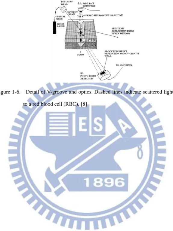
In 1997, Eric Altendorf et al. demonstrating micro-fabricated silicon flow channels to differential counting of lymphocytes, monocytes, red blood cells and platelets by means of laser light scattering [8]. Their measurement system included
7
expensive optical equipment such as optical fiber, diode laser, photo diode detector and PMT detector; they are illustrated in Figure 1-6.
In the developing of fluorescence-based flow cytometry, Li Shi Lim et al. designed a microsieve lab-chip device for rapid enumeration of circulating tumor cells (CTCs) in 2012 [9]. In this search, CTCs could be separated from whole blood and be counted by fluorescence method. But it included time consuming process - antibody staining and counted the cells under fluorescence imaging.
8
Figure 1-6. Detail of V-groove and optics. Dashed lines indicate scattered light due to a red blood cell (RBC).[8]
9
1-4 The applications of micropores
Micro-pores device had a widespread application. They could be used in particle-sorting [10], cell trapping and cells enumeration etc.
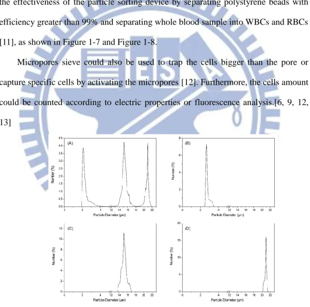
In 2010, Huibin Wei et al. took porous membrane as particle-sorting device. They separated polystyrene beads with different diameter by the device. The beads bigger than the pores would be trapped on the membrane, on the contrary the smaller beads would pass through the membrane. Based on the principle, they demonstrated the effectiveness of the particle sorting device by separating polystyrene beads with efficiency greater than 99% and separating whole blood sample into WBCs and RBCs [11], as shown in Figure 1-7 and Figure 1-8.
Micropores sieve could also be used to trap the cells bigger than the pore or capture specific cells by activating the micropores [12]. Furthermore, the cells amount could be counted according to electric properties or fluorescence analysis.[6, 9, 12, 13]
Figure 1-7. Sorting results for different sizes of PS particles. (A) Particle mixture measurement before sorting; (B), (C), and (D) measurement of the smallest, intermediate and largest collected particles, respectively.[12]
10
Figure 1-8. Sorting results of whole blood. (A) Particle distribution measurements of whole blood before sorting; (B) particle distribution measurements of collected red blood cells and platelets; and (C) collected white blood cells and REH cells.[12]
11
1-5 The electrical circuit model of micropore
Our measurement system and device can be represented by an electrical circuit model consisting of pore resistance, Rp, in parallel with a membrane capacitance, CM, and they series with electrolyte resistance, Rel [14]. The schematic model of the circuit is illustrated at Figure 1-9.
Figure 1-9. The schematic model of the circuit.
1-5-1 Pore resistance
The resistance of the pore is equal to the integral of the resistance along the path of ions flow. Besides the resistance within the pore, any measurement would include the access resistance on both sides. The concept was first brought up in 1968 by Hille [15]. When the ratio of pore length to pore diameter is below 0.05, the Rac will dominate the total pore resistance [16]. In our device, the ratio of pore length to diameter is about 0.07, the access resistance would contribute an obvious part in pore resistance. In the following computing, access resistance will take into account.
12
The resistance within the pore, in the other hand, the channel resistance, Rch can be described as below.
The access resistance, Rac on each side was displayed as below.
ρ : the resistivity of the aqueous medium L : the length of the pore
r : the radius of the pore
Total pore resistance, Rp is the sum of channel resistance and access resistance at both sides, and it could be describe as below.
And the simplified circuit was shown in Figure 1-10 [17].
Figure 1-10. Total channel resistance is a sum of the resistance of the channel proper and access resistances at both sides of the channel.[17]
1-5-2 Membrane capacitance
Every layer of the structure will contribute a capacitance. The value of membrane capacitance is in inverse proportion to the membrane thickness.
13
1-5-3 Electrolyte resistance
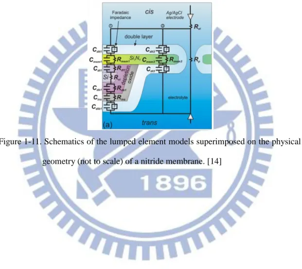
In our measurement system, the resistance we have measured is not only including pore resistance but also including electrolyte resistance which in series with the pore resistance, as shown in Figure 1-11. Electrolyte resistance, Rel, is inflected by the resistivity of the aqueous medium, ρ and the distance between two reference electrodes.
Figure 1-11. Schematics of the lumped element models superimposed on the physical geometry (not to scale) of a nitride membrane. [14]
14
1-6 Motivation 1-6-1 Motivation
Cell counting is an important topic in biology and medicine field and is widely applied in clinic diagnosis. There are many methods in cells counting, but some of them are too expensive, time-consuming or not accuracy enough. Moreover, current hemocytometer can not support cell counting when the cell concentration is lower than 103/ml. In this study, we expect to design a rapid, cheap and accurate measurement system to count cell by combining the micro-pore sieve device and electrical property measurement system.
1-6-2 Goal of this study
In previous research, the micro-pore sieve could be used to sort cells by size. The cells which are bigger than the pore would be trapped on the sieve. As the micropores are blocked by the cells or beads, the resistance of the pore would increase. Once measuring the resistance across to the pore, we could infer whether the pores are blocked or not from the electric information.
In this research, we will combine the micro-pore sieve and electric property measurement system to detect the concentration of polystyrene beads and HeLa cells. Inject the sample with a constant rate into the micro-fluidic channel, the rate of all the micropores be filled will difference with the sample concentration. We will analysis the measurement effect of different pore number from the results and find out the best one. We expect to detect the sample concentration within 2min and sensitive enough to detect the concentration of 100 cells / ml.
15
Chapter 2
Device Preparation
2-1 Device fabrication process
In this research, we applied a convenient micro-fabrication process. These processes took place in National Chiao Tung University Nano Facility Center (NFC). And the following equipment were used: Wet bench, Low pressure chemical vapor deposition system (LPCVD), Vacuum oven, Photoresist spinner, Optical microscope, Double side mask aligner and Dielectric material reactive ion etching system (RIE 200L). The fabrication process was described below.
2-1-1 Silicon wafer clean
In this experiment, double side polished (110) silicon wafers with 250 µm thickness were used. These wafers were cleaned in the following process:
H2SO4 : H2O2 = 3 : 1 in 75 ℃ for 10 min DI water rinse for 5 min
HF : H2O = 1 : 100 in room temperature until the surface is hydrophobic. DI water rinse for 5 min
NH4OH : H2O2 : H2O = 1 : 4 : 20 in 75 ℃ for 10 min DI water rinse for 5 min
HCl : H2O2 : H2O = 1 : 1 : 6 in 75 ℃ for 10 min DI water rinse for 5 min
HF : H2O = 1 : 100 in room temperature until the surface is hydrophobic. DI water rinse for 5 min
Because the wafer is too slight to stand high stress, after the clean process, we used nitride air gun to blow away the residual water instead using spin dryer. Then, baking the silicon wafer in 150 ℃ for 10 min to take out the residual moisture.
16
2-1-2 Silicon nitride deposition
Low stress silicon nitride was deposited by Low Pressure Chemical Vapor Deposition (LPCVD) system. The wafers was put into the furnace, then, rising the furnace temperature to 825 ℃. After the temperature was rose to the assigned temperature, importing NH3 and SiH2Cl2 at the flow rate of 17 sccm and 85 sccm for 90 min to deposit 500 nm low stress nitride.
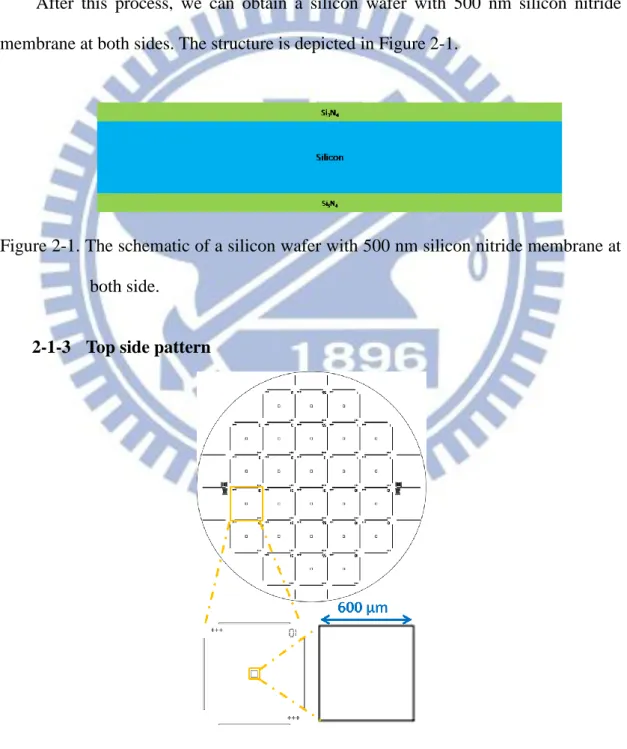
After this process, we can obtain a silicon wafer with 500 nm silicon nitride membrane at both sides. The structure is depicted in Figure 2-1.
Figure 2-1. The schematic of a silicon wafer with 500 nm silicon nitride membrane at both side.
2-1-3 Top side pattern
17
In order to obtain a region of silicon nitride membrane in which length and width are both excess 200 µm on the bottom side after wet etching, we opened square windows with 600 µm in length on the top side as show in Figure 2-2.
First, coat HMDS to improve the adhesion between the silicon wafer and photoresist. After that, coat positive photoresist (FH 6400) by spinner. The first step rotation rate is 500 rpm for 10 sec; the second step rotation rate is 2500 rpm for 25 sec. Then, soft bake at 95 ℃ for 90 sec. Expose the photoresist under light intensity 130 millijoule per square centimeter. Development by the developer (FHD-5) for 20 sec. Hard bake at 120 ℃ for 90 sec.
After pattering the photoresist, the silicon nitride was etched by Dielectric Materials Reactive Ion Etching System (RIE 200L). We infused O2 and CF4 into the chamber at the flow rate of 80 sccm and 20 sccm as reactive gas. The reaction time is 400 sec to remove the 500 nm silicon nitride.
Last, soak the wafer in acetone 10 min to dissolve the photoresist. The wafers cannot be shaken by ultrasonic oscillator because the wafer would break during this
process.
After this process, we can obtain a silicon nitride membrane with a square on it
as depicted at Figure 2-3.
Figure 2-3. The schematic of the wafer after dry etching, there’s a square on silicon
18
2-1-4 Bottom side pattern
Figure 2-4. The bottom side mask pattern.
There were different quantities of the micro-pores designed on the bottom side mask. The pore size is 7 µm in diameter with 14 µm pitch as show in Figure 2-4. Difference pore number were designed, they are 9,49, 100, 484 individually as show in Figure 2-5.
Figure 2-5. Design of different pore numbers on the mask.
The following steps to define the bottom side silicon nitride pattern are similar with the top side pattern process. After this process, we can obtain a silicon nitride
19
membrane with micropore array, and the pore sizes and pore quantities are the same
with the mask. The cross sectional schematic was depicted at Figure 2-6.
Figure 2-6. The schematic of silicon nitride membrane with micropore array.
2-1-5 Wet etching
To etch the spare silicon between the membranes we dipped the silicon wafer into 30 wt% KOH solution at 80 ℃ for 5 hours. In order to let the surface be smoother, 4 % isopropyl alcohol (IPA) was added into the solution. This solution would anisotropy etch the silicon, the etch rate for (111) plane is remarkable slower than other planes. So there would be a trapezoid chamber in the silicon wafer after the etching process as illustrated in Figure 2-7.
20
2-2 Device analysis
The micropore devices were examined by SEM and OM to confirm the consistence to the design. After that, pore diameter was analyzed by ImageJ and Si3N4 membrane thickness was characterized by N&K analyzer.
2-2-1 SEM and OM image
Figure 2-8(a) is optical microscope (OM) image of the device. From the image, it could be know that the top side pattern and bottom side pattern had been aligned together; the micro-pores array is located at the center of the silicon fillister dug in the wet etching process. To inspect more detail of the device, it was examined under scanning electron microscope (SEM). It could be confirmed that there are micro-pores array channels located on the silicon nitride membrane. The SEM image is shown in Figure 2-8 (b).
(a) (b)
Figure 2-8. The optical microscope and scanning electron microscope image of the device. Scale bar: 10 m.
2-2-2 Membrane thickness analysis
After the silicon nitride membrane deposition process, we would measure the membrane thickness first. The measurement was carried out by the N&K analyzer possessed in National Nano Device Laboratories (NDL).
21
center of the wafer and the interval between points is 3 centimeter as shown in Figure 2-9. The average thickness is 505 ± 26.5 nm according to the statistical result.
Figure 2-9. The positions of silicon nitride thickness measurement points.
2-2-3 Pore diameter analysis
Since the pore diameter would be little inaccuracy in the process of exposure, develop and dry etching, it should be reconfirmed. ImageJ was applied to analyze the diameter the result shows that the average pore diameter is 6.68 ± 0.39 μm.
22
2-3 Cell culture process
HeLa cells were used in this research to demonstrate the cell counting. Cells were cultivated in the medium containing 90% DMEM medium and 10% newborn calf serum. We displaced the medium to trypsin and put the dish into incubator for 2 min to separate the cells from the dish. Then, add the medium had been mention previous into the dish and draw out all the solution to centrifugal tube. Put the centrifugal tube into centrifuge; adjust the rotation rate at 1500 rpm for 3 min; draw out the solution and keep the HeLa cells in the tube. At last, add 1X PBS into the tube and adjust the cell concentration. Before measuring the concentration by micropores sieve, we applied hemocytometer to estimate the cell concentrations.
23
2-4 Polystyrene beads sample preparing process
In order to carry out the research more convenient, we used polystyrene beads instead of cells to demonstrate the experiment. Nonionic white polystyrene latex was purchased from InvitrogenTM. The size of the polystyrene beads is 10 ± 0.63 µm in diameter. Polystyrene beads dissolved in DI water and the concentration is 7.4 × 10⁷ beads/ml.
The polystyrene beads solution was diluted with various volume ratios of 0.1M KCl. We diluted the polystyrene beads into 1.5 × 10², 1.5 × 10³, 1.5 × 10⁴, 1.5 × 10⁵ and 1.5 × 10⁶/ml in concentration. And use hemocytometer to re-confirm the concentration. But from the image of hemocytometer, we could only recognize the concentration from 106 to 104 / ml. So the other concentrations were diluted from the sample with a know concentration.
Figure 2-11. The image of hemocytometer for 1.5 × 10⁶ beads/ml solution.
24
Figure 2-13. The image of hemocytometer for 1.5 × 10⁴ beads/ml solution.
25
2-5 Acrylic block design
There was a T-shaped channel inside the acrylic block as showed in Figure 2-16. And the dimensions are shown in Figure 2-15. One side of the channel was the inlet that let the sample solution flow in, anther side was used to fix the Ag/AgCl reference electrodes and the other was aligned with the micropores array to let the sample flow through the chip.
Figure 2-15. The lateral view of the acrylic block.
26
2-6 Microfluidic Fixture
Materials:
Acrylic block mention in chapter 2-5 × 2
O-ring with internal diameter 3.6 mm and external diameter 6.2 mm × 2 O-ring with internal diameter 1.2 mm and external diameter 3.2 mm × 2 Ag/AgCl reference electrode × 2
Teflon tube in 10 centimeter × 2 Micro-sieve device × 1
Syringe × 1
Screws and nuts × 2
PDMS with thickness 0.8 mm and a hole with diameter 1 mm × 2 Difference concentrations beads solution × 500 µl
The micro-sieve was clipped between two acrylic blocks which had a 1 mm hole aligned with the micro-pores array. To avoid the solution leaking from cracks, we put the PDMS between the acrylic blocks and the micro-sieve device and plugged the O-rings in the channel terminal. The Ag/AgCl reference electrodes were inserted into the acrylic blocks and put an O-ring around it to avoid solution leaking. The sample solution was loading in a syringe which connecting to a Teflon tube and the tube was inserted into the inlet channel. And the set up would be fixed by screws and nuts. The sketch was depicted in Figure 2-17.
27
Figure 2-17. The photograph of the microfluidic channel including the arcrylic fixture.
The sample solution was injected into the channel and passed through the pores by the syringe pump in a constant flow rate. Ag/AgCl reference electrodes were inserted into the flow channel and connected to the lock-in amplifier (SR-850) to measure the ion-current.
28
2-7 Set-up of Measurement equipment
The voltage was applied via a lock-in amplifier (SR850) by connecting to the reference electrodes. The data acquisition was fulfilled via a DAQ card and a computer.
29
Chapter 3
Equivalent Circuit
3-1 Theoretic value of pore resistance and device resistance
According to the formula and electrical circuit model that have be mentioned in section 1-5, the theoretic values of Rac, Rch and Rp can be estimated through measurement. The influence of pore geometry on resistance is remarkable. From previous experiments, the pore diameter and membrane thickness is 6.68 ± 0.39 μm and 505 ± 26.5 nm individually. The resistivity of 0.1 M KCl is 0.775 •m.
3-1-1 Maximum and minimum value of pore resistance
The dimensions of micropores are not so precise that exist an error amount. And this magnitude of the error is large enough to influent the resistance. In the computation minimum pore resistance process, we assumed the diameter of the pore is 7.07μm; the thickness of the pore is 478.5 nm.
Access resistance is equal to ρ and channel resistance is equal to ρ , substituting r for 3.535μm, L for 478.5 nm and ρfor 0.775 m. The result is displayed as below. Minimum RP: ρ ρ In the computation maximum pore resistance process, we assumed the diameter
30
of the pore is 6.29 μm; the thickness of the pore is 531.5 nm. Substitute r for 3.145μm, L for 531.5 nm and ρfor 0.775 m. The result is displayed as below.
Maximum RP: ρ
3-1-2 Device resistance for single pore and multiple pores
The circuit model of the single pore device is depicted at Figure 3-1. Pore resistance is parallel with membrane capacitance, and they series with electrolyte resistance. According to the computation result, we know Rp is between the ranges of 119.064 k to 136.466 k. Electrolyte resistance value could be derived from the impedance measurement result; it is between the ranges of 10 k to 13 k. Total resistance, RT, is the sum of Rel and RP.
Figure 3-1. The equivalent circuit model for single pore device.
The simplify circuit model of multiple pores device is illustrated at Figure 3-2. Every Rp is parallel with CM, and they parallel to each other. As the result of Rp is
31
parallel to each other, the device resistance, RD, would decrease with the pore number increase. Device resistance could be expressed as below.
Take the 9 pores device for example, device resistance, RD, could be calculated as below. Minimum RD: Maximum RD:
From the computation result, RD in 9 pores device is ranging from 13.22 k to 15.11 k. Apply the same rule on other device, we could know RD is ranging from 2.43 k to 2.78 k for 49 pores device; 1.19 k to 1.36 k for 100 pores device, 0.26 k to 0.28 k for 484 pores device, as displayed in
32
Figure 3-2. The schematic of equivalent circuit model for multiple pores device.
Table 3-1. The theoretic value of device resistance for different devices.
Pore number RD (k) 1 119~136 9 13.22~15.11 49 2.43~2.78 100 1.19~1.36 484 0.26~0.28
33
3-2 Massurement of pore resistance and device resistance
After calculating the value of RD and Rp, a practical measurement was carried out by an impedance analyzer (BioLogic, VSP-300).The impedance was measured from 1 Hz to 1M Hz. And the value of electrolyte resistance, device resistance and membrane capacitance were characterized.
3-2-1 Micro-pores device characteristic analysis
Figure 3-3 shows the impedance measurement result. The impedance in low frequency is about 38.49 k for 9 pores sieve, 19.86 k for 49 pores sieve, 18.33 k for 100 pores sieve, 12.73k for 484 pores sieve. The impedance at high frequency is between 9 k from 12 k for all devices.
Figure 3-3. The impedance of different device.
Applying the impedance formula and Nyquist Diagram ( -Im|Z| vs. Re|Z| ), we can analyze the value of Rel, RD and QM by EC-Lab software. The Nyquist Diagram
34 Table 3-1.
Figure 3-4. The Nyquist diagram and curve fitting of 9 pores device.
Figure 3-5 The Nyquist diagram fitting curve of 49 pores device.
35
Figure 3-7. The Nyquist diagram and curve fitting of 484 pores device.
Table 3-2 The actual value of electrolyte resistance and device resistance.
Pore number Rel (k) RD (k) QM (F) a
9 11.169 27.320 2.040 × 10⁻⁹ 0.884
49 10.684 9.174 3.952 × 10⁻⁹ 0.791
100 11.956 6.375 6.869 × 10⁻⁹ 0.790
484 9.675 3.058 1.363 × 10⁻⁹ 0.852
3-2-2 Micro-pores device with polystyrene beads measurement
To understand the variation of RD after the pores be blocked by polystyrene beads, the solution with polystyrene beads was injected into the chamber until all the pores are blocked. And measure the impedance again.
Figure 3-8 and Figure 3-9 are the impedance spectra and Nyquist diagram and the curve fitting for 49 pores device with blocked pores. From the analysis result, it could be know that the impedance in low frequency increased from 19.89 k to 27.76 k. But the impedance in high frequency is about the same.
36
Figure 3-8. The impedance measurement curve for 49 pores device when all the pores are blocked.
Figure 3-9. The Nyquist diagram and curve fitting of 49 pores device when the all the pores are blocked.
Compare the impedance of the pores be blocked and unblocked, RT increase from 19.89 k to 27.76 k, Rel is almost remained the same, RD increase from 9.174 k to 17.057 k. It could be known that when the pores are blocked, RD increases by 2 times. The results are shown in Figure 3-10 and Table 3-3.
37
Figure 3-10. The impedance before and after the pores be blocked for 49 pores device.
Table 3-3 Compare of device resistance before and after the pores be blocked for 49 pores device
Pore status Rel (k) RD(k) QM (F) a
Pores are unblocked 10.684 9.174 3.952 × 10⁻⁹ 0.791
Pores are blocked 10.707 17.057 2.006 × 10⁻⁹ 0.876
.
3-2-3 Consideration in pore number
Table 3-3 shows that Rel won’t change and RD would increase by 2 times when the pores are blocked. As the results show by Table 3-2, the fewer of pores, the larger i s the ratio of RD to RT. Apply the same concept, the larger of the pore quantity, the smaller of the RT variance could be measured when the pores are blocked. In order to obtain a noticeable resistance variation, the devices with fewer pore numbers are chosen.
38
3-3 Frequency effect
In our measurement, we could obtain the impedance value. The impedance would vary with frequency, f. The impedance, Z, could be written as below.
In high frequency, the latest item of above-mentioned formula would approach to zero. So the impedance would approach to Rel. In low frequency, the latest item of above-mentioned formula would approach to RD. Therefore the impedance would approach to Rel + RD.
High frequency :
Low frequency :
In this research, device resistance, RD, is the main parameter to help us infer the pore status, so the experiments were operated at low frequency.
39
3-4 Working Frequency
To improve the results in chapter 3-3, I took the experiments in low frequency and high frequency respectably. Use the 9 pore device, the ionic current curve in low frequency was distinct from in high frequency when the polystyrene beads are trapped on the pores.
In low frequency, when every bead was trapped on the sieve, the ionic current would decrease obviously and there would result in a step in the curve. On the contrary, when every bead was trapped on the sieve in high frequency, the ionic current remains in a consistent. The experiment results are shown in Figure 3-11 and Figure 3-12. These phenomena tally with what predicted in chapter 3-3. The pore status could be inferred by monitoring the current in low frequency.
In addition, from the impedance measurement result it could prove that the impedance measuring in high frequency equal to Rel. As shown in Figure 3-13, in high frequency, the impedance values of different device are similar. It cause from the electrolyte resistance is independent of the pore number. But in low frequency, the impedance would vary with pore number, because the impedance equal to the sum of Rel + RD in this situation.
40
Figure 3-11. In low frequency (10 Hz), when every bead was trapped on the sieve, the ionic current would decrease obviously and there would result in a step in the curve.
Figure 3-12. In high frequency (50 kHz), when every bead was trapped on the sieve the ionic current remains in a consistent.
41
42
Chapter 4
Results and Discussion
4-1 Current drop caused from polystyrene beads 4-1-1 49 pores device
The experiment was manipulated in following conditions: applied voltage with 10 mV in 10 Hz, used the device with 49 pores, and injected the sample with concentration of 106 beads / ml at the rate of 20 µl / min. In addition, the status of the pores was recorded under optical microscope simultaneously. The measurement result is shown in Figure 4-1. The current kept in horizontal at the initial 14 seconds, dropped abruptly from 14th to 20th second, at last, the pores were saturated and the curve slope turned gently at about 20th second. Based on these difference phenomena, the curve was divided into three regions as shown in Figure 4-1.
In region Ⅰ, the polystyrene beads were not yet arrived to the micro-pores sieve(Figure 4-2), RP value was not change, so the current kept in constant. Figure 4-3 indicated that the micropores were blocked by polystyrene beads gradually from the 14th to 22nd second. Therefore, Rp and RD increased and the ionic current decreased. This phenomenon conformed to that indicated in region Ⅱ of Figure 4-1. Therefore, a conclusion could be judged that the ionic current drop is the result of the micropores are blocked by polystyrene beads.
4-1-2 9 pore device experiment
In the same condition, but replaced 49 pores device by 9 pores device to repeat the experiment. As shown in Figure 4-5 and Figure 4-6, when every bead was trapped on the sieve, the ionic current decreased obviously and resulted in a step in the curve. And if there were not any bead be trapped on, the current curve kept in constant. It proof again that the current drop was caused by polystyrene beads be trapped on.
43
Furthermore, we can know the beads quantity by counting the amount of steps in Figure 4-5. Every step represents one bead. When the amount of pores increase the current variation caused by every individual beads will decrease. Like the current curve shown in Figure 4-1, the current variation caused by one bead blocking is so small that there are not obvious step observed but a smooth descending curve.
Saturation time
Figure 4-1. The ionic current curve in following measurement conditions : applied voltage with 10 mV in 10 Hz, used the device with 49 pores, injected the sample with concentration of 106 beads/ml at the rate of 20 µl/min.
44
Figure 4-2. The OM image in region I of Figure 4-1.
Figure 4-3. The OM image in region II of Figure 4-1.
45
Figure 4-5. The ionic current curve in following measurement conditions: applied voltage with 10 mV in 10 Hz, used the device with 9 pores, injected the
sample with concentration of 104 beads/ml at the rate of 20 µl/min.
Figure 4-6. The OM image corresponds. Every figure corresponds to the time labbeld in Figure 4-5.
46
4-2 Beads measurement results and discussion
The previous experiment results and the simulation electrical circuit model indicated that the micro-pore impedance variation cause from the pore be blocked by beads in low frequency would more obvious than in high frequency. So in following experiment, low frequency – 10 Hz was chosen and the applied voltage is 10 mV. All the beads were dissolved in 0.1 M KCl which has similar conductance with 1X PBS. The beads were composed by polystyrene with 10 ± 0.63 μm in diameter. The sample solution was injected into the flow channel by syringe pump in the flow rate of 20 µl / min. Pure 0.1 M KCl without polystyrene beads was injected in the initial 10 seconds, the sample solution that contain different concentration of polystyrene beads was injected form the 10th second.
In the following experiments, we used difference pore number micropores sieve device to detect the beads concentration. The pore number ranged from 1 to 484, and we expected to distinguish the beads concentration from 102 beads/ml to 106 beads /ml.
4-2-1 Resolving of bead concentrations
Apply the value in Table 3-2 and Table 3-3, it could be estimated that the ionic current might decline to 84% or lower after the polystyrene solution had injected when using 484 pores device.
47
difference concentration samples. Once polystyrene beads arrive the device and block the micro-pore channels, the ionic current will start to decrease. The variations of the ionic current in 102 to 104 beads / ml are almost the same in the initial 100 seconds. Because the pore blocked rate is too low and the variations are smaller than the error amount so it couldn’t be distinguished. But the variation could be distinguished between 104 to 106 beads /ml, as shown in Figure 4-12.
Apply the value in Table 3-2 and Table 3-3, it could be estimated that the ionic current might decline to 77% or lower after the polystyrene solution had injected when using 100 pores device.
Figure 4-13 to Figure 4-17 are the results that applied 100 pores device to detect difference concentration samples. Once polystyrene beads arrive the device and block the micro-pore channels, the ionic current will start to decrease. The variation of ionic current at 100th second could be distinguished from 102 to 106 beads /ml, as shown in Figure 4-18.
Apply the value in Table 3-2 and Table 3-3, it could be estimated that the ionic current might decline to 71% or lower after the polystyrene solution had injected when using 49 pores device. Figure 4-19 to Figure 4-23 are the results that applied 49 pores device to detect difference concentration samples. Once polystyrene beads arrive the device and block the micro-pore channels, the ionic current will start to decrease. The variation of ionic current at 100th second could be distinguished from
48 102 to 106 beads /ml, as shown in Figure 4-24.
Apply the value in Table 3-2 and Table 3-3, it could be estimated that the ionic current might decline to 60% or lower after the polystyrene solution had injected when using 9 pores device.
49
Table 4-1 The actual value of electrolyte and device resistance for 484 pores device.
Pore number Rel (k) RD (k) CM (F) RT (k)
484 10.171 2.502 0.199 × 10 -9 12.673
Current variation rate: RT / (RT + RD) = 84%
Figure 4-7. The current decline curve for 102 beads/ml sample by 484 pores device.
Figure 4-8 The current decline curve for 103 beads/ml sample by 484 pores device.
Figure 4-9 The current decline curve for 104 beads / ml sample by 484 pores device.
Figure 4-10 The current decline curve for 105 beads/ml sample by 484 pores device.
Figure 4-11 The current decline curve for 106 beads/ml sample by 484 pores device.
Figure 4-12 The statistics of different concentrations for 484 pores device.
50
Table 4-2 The actual value of electrolyte and device resistance for 100 pores device.
Pore number Rel (k) RD (k) CM (F) RT (k)
100 12.139 5.058 0.692 × 10 -9 17.197
Current variation rate: RT / (RT + RD) = 77%
Figure 4-13 The current decline curve for 102 beads / ml sample by 100 pores device.
Figure 4-14. The current decline curve for 103 beads / ml sample by 100 pores device.
Figure 4-15. The current decline curve for 104 beads / ml sample by 100 pores device.
Figure 4-16 The current decline curve for 105 beads / ml sample by 100 pores device.
Figure 4-17. The current decline curve for 106 beads / ml sample by 100 pores device.
Figure 4-18. The statistics of different concentrations for 100 pores device.
51
Table 4-3 The actual value of electrolyte and device resistance for 49 pores device.
Pore number Rel (k) RD (k) CM (F) RT (k)
49 11.628 8.015 0.320 × 10⁻⁹ 19.643
Current variation rate: RT / (RT + RD) = 71%
Figure 4-19. The current decline curve for 102 beads /ml sample by 49 pores device.
Figure 4-20. The current decline curve for 103 beads /ml sample by 49 pores device.
Figure 4-21. The current decline curve for 104 beads/ml sample by 49 pores device.
Figure 4-22. The current decline curve for 105 beads / ml sample by 49 pores device.
Figure 4-23. The current decline curve for 106 beads / ml sample by 49 pores device.
Figure 4-24. The statistics of different concentrations for 49 pores device.
52
Table 4-4 The actual value of electrolyte and device resistance for 9 pores device.
Pore number Rel (k) RD (k) CM (F) RT (k)
9 11.757 26.096 0.551 × 10⁻⁹ 38.853
Current variation rate: RT / (RT + RD) = 60%
Figure 4-25. The current decline curve for 102 beads /ml sample by 9 pores device.
Figure 4-26. The current decline curve for 103 beads / ml sample by 9 pores device.
Figure 4-27. The current decline curve for 104 beads / ml sample by 9 pores device.
Figure 4-28. The current decline curve for 105 beads /ml sample by 9 pores device.
Figure 4-29. The current decline curve for 106 beads/ml sample by 9 pores device.
Figure 4-30. The statistics of different concentrations for 9 pores device.
53
4-2-2 Discussion
From the calculation results, we could know that when the all the micropores are blocked (saturate), the ionic current will drop to 71% of initial value for 49 pores device and 77% for 100 pores device. And the saturation time will different with the concentrations. By analyzing the saturation time, the sample concentration could be known. In Figure 4-31 and Figure 4-32 displayed the saturation time for 49 and 100 pores device of different concentration. Both of the curve showed that the lower of the concentration the longer of the saturation time, based on this concept, the concentration could be distinguished from 102 to 106 beads /ml. In addition, the detection time for 49 pores device is about 300 seconds and 100 pores device is about 450 seconds. Using the device with fewer pores can speed up the detection rate.
54
Figure 4-32. The saturation time for 100-pore device of different concentration.
In order to accelerate the detection rate, the ionic current values in specific time were compiled. The ionic current values at 50 s, 100 s and 150s after starting the measurement are indicated as Figure 4-33 to Figure 4-35. At 100th and 150th second, it could distinguish the concentration from 102 to 105 beads/ml by 49 pores device and distinguish the concentration from 103 to 106 beads/ml by 100 pores device. The sample concentration could be known within 2 min by applying this statistical method.
55
Figure 4-34. The ionic current values at 100 s after the measurement started.
56
4-3 Concentration of HeLa cells
From the conclusion of the beads experiments, we know that 49 pores micro-sieve device is more sensitive and faster to detect the beads concentration in the range from 102 to 106 beads/ml. So we used it to demonstrate the cells experiment. Before the measurement, the HeLa cells concentration would be confirmed by the hemocytometer. The sample with concentration lower than 104 cells / ml could not be confirmed by it, we could only dilute the higher concentration sample with 1X PBS to obtain.
From the ionic current curve shown in Figure 4-36, it is obvious that different concentration’s curve has different slope. By analyzing the ionic current value at specific time, the concentration could be known.
In addition, HeLa cells measurement results are compared with polystyrenes’. The tendency of the former is coincident with the latter, as shown in Figure 4-37.
57
Figure 4-37. The comparison of polystyrene beads and HeLa cells measurement results by using the 49-pore device. The current ratio at 100th second after starting the measurement.
58
Chapter 5
Conclusion and future work
5-1 Conclusion
In this research, cell concentration could be detected rapidly by measuring the ionic current across to a silicon nitride membrane with micropores array. Difference from previous researches, cells concentration could be known in a short time and it could be done without expensive equipment in this measurement method.
From these experiments, we could obtain the conclusions as following:
1. The device with 49 pores has the best sensitivity of polystyrene bead and HeLa cell concentration. And the device with 484 pores is more suitable in high concentration; the device with 9 pores is more suitable in low concentration. 2. Every bead be caught by the 9 pores device could be recognized. Base on the
phenomena, 9 pores device could use to count the beads.
3. The concentration of polystyrene beads from 102/ml to 106/ml could be distinguished by silicon nitride micropore sieve device.
4. The concentration of HeLa cells from 102/ml to 106/ml could be distinguished by silicon nitride micropore sieve device.
59
5-2 Future work
To improve the efficiency of this micropore sieve measurement system, the following experiments are suggested to be carried out.
1. Improve the fluidic channel and reduce the chamber volume to speed up the detection rate.
2. Apply the size selective effect to separate difference cells and detect the concentrations individually.
3. Modify biomolecules on the micropores to catch specific cells and detect the concentration.

![Figure 1-1. Schematic of a Hemocytometer. [18]](https://thumb-ap.123doks.com/thumbv2/9libinfo/8559630.188444/17.892.136.796.356.884/figure-schematic-hemocytometer.webp)
![Figure 1-2. Schematic of a Coulter counter. [19]](https://thumb-ap.123doks.com/thumbv2/9libinfo/8559630.188444/19.892.167.700.105.937/figure-schematic-of-a-coulter-counter.webp)
![Figure 1-10. Total channel resistance is a sum of the resistance of the channel proper and access resistances at both sides of the channel.[17]](https://thumb-ap.123doks.com/thumbv2/9libinfo/8559630.188444/26.892.134.754.325.927/figure-total-channel-resistance-resistance-channel-resistances-channel.webp)
![TraditionalMLCalgorithmsmainlytacklethebatchMLCproblem,wheretheinputdataarepresentedinabatch[24,28].Nevertheless,inmanyMLCapplicationssuchase-mailcategorization[22],multi-labelexamplesarriveasastream.Onlineanalysisistherefore dimensionreducermotivatedbyma](data:image/gif;base64,R0lGODlhAQABAIAAAP///wAAACH5BAEAAAAALAAAAAABAAEAAAICRAEAOw==)