應用可變結構控制技術於反戰術彈道飛彈具有側向力與氣動力之複合控制技術之研究

國

立

交

通

大

學

電控工程研究所

碩士論文

應用可變結構控制技術於反戰術彈道飛彈

具有側向力與氣動力之複合控制技術之研究

Application of Variable Structure Schemes to the Control of

Anti-Tactical Ballistic Missile Having Lateral Thrust and

Aerodynamic Forces

研 究 生：康詠鈞

指導教授：梁耀文 博士

中 華 民 國 一 百 零 二 年 七 月

應用可變結構控制技術於反戰術彈道飛彈

具有側向力與氣動力之複合控制技術之研究

Application of Variable Structure Schemes to the Control of

Anti-Tactical Ballistic Missile Having Lateral Thrust and

Aerodynamic Forces

研 究 生：康詠鈞

Student： Yung-Chun Kang

指導教授：梁耀文 博士 Advisor： Dr. Yew-Wen Liang

國立交通大學電控工程研究所

碩士論文

A Thesis

Submitted to Institute of Electrical Control Engineering

College of Electrical Engineering and Computer Science

National Chiao Tung University

in Partial Fulfillment of the Requirements

for the Degree of Master

in

Electrical and Control Engineering

July 2013

Hsinchu, Taiwan, Republic of China

應用可變結構控制技術於反戰術彈道飛彈

具有側向力與氣動力之複合控制技術之研究

研究生：康詠鈞

指導教授：梁耀文 博士

國立交通大學電控工程研究所

摘 要

本論文的主要目的在探討具有氣動力和側向力的反戰術彈道飛彈之複合控制

技術。由於科技的不斷發展，目標飛彈的機動性不斷提升，為了在攔截末段實現

直接碰撞高機動性目標飛彈的攔截任務，複合式控制的概念油然而生，取代傳統

僅依賴氣動力控制的飛彈。相對於純尾翼控制，複合控制具有如下之特點：

1) 系

統時間響應速度快；2) 側向力不受海拔高度影響；3) 複合控制能降低側向力的

能量消耗並且提升系統的追蹤性能表現。本論文首先建立複合式的反戰術彈道飛

彈六自由度數學模型，並探討應用三種可變結構控制技術：1) 傳統順滑模控制

(conventional sliding mode control)技術、2) 終端順滑模控制(terminal sliding mode

control)技術與 3) 非奇異終端順滑模控制(nonsingular terminal sliding mode control)

技術在氣動力與側向力的複合控制之性能比較。由模擬結果顯示，除驗證了本文

所設計之控制器的性能表現外，也展示了複合式飛彈的系統響應速度的確比傳統

只使用氣動力的飛彈快，這些模擬具體地說明了複合式飛彈未來發展的潛力。

Application of Variable Structure Schemes to the Control

of Anti-Tactical Ballistic Missile Having Lateral Thrust

and Aerodynamic Forces

Student: Yung-Chun Kang Advisor: Dr. Yew-Wen Liang

Institute of Electrical Control Engineering

National Chiao Tung University

ABSTRACT

This thesis studies the control of anti-tactical ballistic missiles (ATBM) having

lateral thrust and aerodynamic forces, called blended control. With increasing

technological sophistication, the maneuverability of tactical ballistic missiles is

improving. Compared with tail control, the blended control possesses the following

three features: 1) timing response is faster; 2) lateral thrust is independent of altitude;

and 3) tracking performance is promoted. In this thesis, we first build the mathematical

model of ATBM and then import the following three variable structure schemes (VSS):

1) conventional sliding mode, 2) terminal sliding mode and 3) nonsingular terminal

sliding mode to the blended control design task. Simulation results clearly demonstrate

the performances of the presented three SMC schemes and confirm that the performance

by blended control is superior to that by the tail control only.

誌 謝

本篇論文的完成，實在要感謝許多人的關心與協助，沒有你們恐怕無法有所精進， 希望日後能繼續給與指教與鼓勵，必銘記在心。 首先特別要感謝指導教授梁耀文博士，感謝老師兩年來細心與耐心的指導及孜孜不 倦的教誨，除了讓我對於控制理論的懵懂漸漸有了體悟與想法，且在人生中待人處事有 許多的不一樣的思維，其中一句：「作而無作，無作而作。」更是深得我心。同時也要感 謝口試委員廖德誠博士、鄭治中博士和徐勝均博士給予建設性的建議與指導，使得本論 文更臻完備。 感謝實驗室的同學們，徐勝均博士、林立岡學長、陳智強學長、馮仰靚學長、陳弘 儒學長及呂鈞鈞學姐，感謝他們在我研究上或學業上有問題時，可以即刻的幫助我，或 是提供我意見。感謝同窗的實驗室同學陳俊宇、陳逸庭與王國欽，感謝他們在一起修課 時互相幫忙，以即互相鼓勵督促。感謝學弟張修維、朱韋銘、吳竣民與洪靜怡，在我需 要幫忙時，適時的給予幫助。感謝我的好友在人生不如意時聽述說痛苦。若無他們的幫 助，我無法完成今天的碩論。 感謝我的女朋友乃慈，在我忙碌時默默地在背後支持我、幫助我、體諒我，使我能 更能專心在學業上衝刺。最後感謝我的家人，由於你們的大力支持與鼓勵，使我在求學 過程中無後顧之憂，如果沒有他們，就沒有今天的我，也就無法完成今天的論文。 康詠鈞 于新竹交大 102 年 7 月

TABLE OF CONTENT

ABSTRACT (Chinese) ……….

i

ABSTRACT (English) ……….

ii

ACKNOWLEDGEMENT

………. iii

TABLE OF CONTENT

………...………... iv

LIST OF FIGURES ………...

vi

LIST OF TABLES

……… ix NOMENCLATURE ... x

1. INTRODUCTION ………... 1

1.1 Motivation ………... 1 1.2 Outline ...……….……… 5

2. PRELIMINARIES ……….. 6

2.1. Conventional Sliding Mode Control (CSMC) …………...……… 6

2.2. Terminal Sliding Mode Control (TSMC) ………. 11

2.3. Nonsingular Terminal Sliding Mode Control (NTSMC) ………. 16

2.4. Mathematical Models of the Missile ……… 20

2.4.1. Coordinate Systems ……….….. 20

2.4.2. Rigid-Body Equations of Motion ……….. 24

2.4.3. Equations of Attitude Dynamics ……… 30

2.4.4. Model of Tail Fins ……….. 33

2.4.5. Reaction-Jet Control System ………. 34

3. OUTPUT TRACKING CONTROL FOR A NONLINEAR SYSTEM ... 36

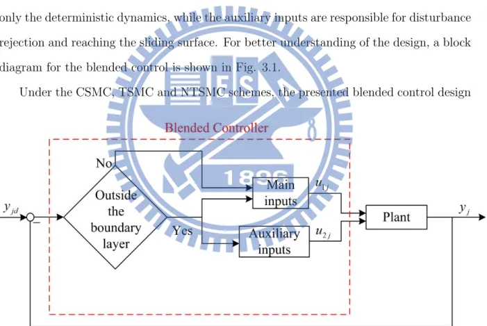
3.1. Problem Formulation ... 36

3.2.1. Control Design via CSMC scheme ... 41

3.2.2. Control Design via TSMC scheme ... 46

3.2.3. Control Design via NTSMC scheme ... 51

4. APPLICATION TO MISSILE SYSTEM ... 56

4.1. Model Description ... 56

4.2. Simulation Results ... 62

5. CONCLUSIONS AND SUGGESTIONS FOR FURTHER REASEARCH ... 86

5.1. Conclusions ... 86

5.2. Suggestions for Further Research ... 87

LIST OF FIGURES

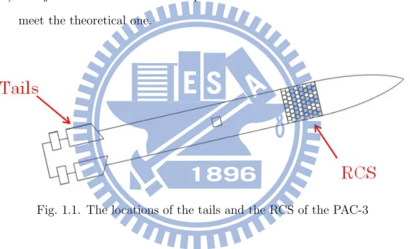
Figure 1.1. The locations of the tails and the RCS of the PAC-3 ... 4

Figure 2.1. A typical phase portrait under sliding mode control ... 7

Figure 2.2. Sliding condition ... 11

Figure 2.3. Chattering as result of imperfect control switchings ... 12

Figure 2.4. The sliding mode of the third-order system ... 13

Figure 2.5. The phase plot of the second-order system ... 19

Figure 2.6. Definitions of



and  ... 21

Figure 2.7. Definitions of



_v ... 22

Figure 2.8. Definitions of



and



_v ... 22

Figure 2.9. Definitions of



,



and



... 23

Figure 2.10. The relationships among coordinates ... 23

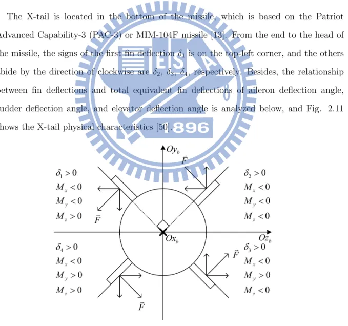
Figure 2.11. Force analysis of X-tail ... 33

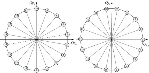
Figure 2.12. The layout scheme of IACMs, left side for odd number and right side for even number ... 35

Figure 3.1. Block diagram of blended control ... 40

Figure 3.2. The time response of s x t_j( ( )) ... 43

Figure 4.1. Time evolution of error e₁ 

 

_d by sign-type SMC scheme ... 68

Figure 4.2. Time evolution of (a)



(b)



_zb (c)



_z by sign-type SMC scheme ... 68

Figure 4.3. Time evolution of the sliding variables by sign-type SMC scheme ... 69

Figure 4.4. Time evolution of



_zc by sign-type SMC scheme ... 69 Figure 4.5. Time evolution of the number of the consumed IACMs by sign-type SMC

scheme ... 70

Figure 4.6. Time evolution of error e₁ 

 

_d by sign-type TSMC scheme ... 70

Figure 4.7. Time evolution of (a)



(b)



_zb (c)



_z by sign-type TSMC scheme ... 71

Figure 4.8. Time evolution of the sliding variables by sign-type TSMC scheme ... 71

Figure 4.9. Time evolution of



_zc by sign-type TSMC scheme ... 72

Figure 4.10. Time evolution of the number of the consumed IACMs by sign-type TSMC scheme ... 72

Figure 4.11. Time evolution of error e₁ 

 

_d by sign-type NTSMC scheme ... 73

Figure 4.12. Time evolution of (a)



(b)



_zb (c)



_z by sign-type NTSMC scheme ... 73

Figure 4.13. Time evolution of the sliding variables by sign-type NTSMC scheme ... 74

Figure 4.14. Time evolution of



_zc by sign-type NTSMC scheme ... 74

Figure 4.15. Time evolution of the number of the consumed IACMs by sign-type NTSMC scheme ... 75

Figure 4.16. Time evolution of the sliding variables in magnified scale by sign-type SMC scheme ... 75

Figure 4.17. Time evolution of the sliding variables in magnified scale by sign-type TSMC scheme ... 76

Figure 4.18. Time evolution of the sliding variables in magnified scale by sign-type NTSMC scheme ... 76

Figure 4.19. Time evolution of error e₁  

 

_d in magnified scale by sign-type SMC scheme ... 77

Figure 4.20. Time evolution of error e₁  

 

_d in magnified scale by sign-type TSMC scheme ... 77

Figure 4.21. Time evolution of error e₁ 

 

_d in magnified scale by sign-type NTSMC

scheme ... 78

Figure 4.22. Time evolution of error e₁ 

 

_d by saturation-type SMC scheme ... 78

Figure 4.23. Time evolution of (a)



(b)



_zb (c)



_z by saturation-type SMC scheme ... 79

Figure 4.24. Time evolution of the sliding variables by saturation-type SMC scheme ... 79

Figure 4.25. Time evolution of



_zc by saturation-type SMC scheme ... 80

Figure 4.26. Time evolution of the number of the consumed IACMs by saturation-type SMC scheme ... 80

Figure 4.27. Time evolution of error e₁ 

 

_d by saturation-type TSMC scheme ... 81

Figure 4.28. Time evolution of (a)



(b)



_zb (c)



_z by saturation-type TSMC scheme ... 81

Figure 4.29. Time evolution of the sliding variables by saturation-type TSMC scheme ... 82

Figure 4.30. Time evolution of



_zc by saturation-type TSMC scheme ... 82

Figure 4.31. Time evolution of the number of the consumed IACMs by saturation-type TSMC scheme ... 83

Figure 4.32. Time evolution of error e₁ 

 

_d by saturation-type NTSMC scheme ... 83

Figure 4.33. Time evolution of (a)



(b)



_zb (c)



_z by saturation-type NTSMC scheme .... 84

Figure 4.34. Time evolution of the sliding variables by saturation-type NTSMC scheme .... 84

Figure 4.35. Time evolution of



_zc by saturation-type NTSMC scheme ... 85

Figure 4.36. Time evolution of the number of the consumed IACMs by saturation-type NTSMC scheme ... 85

LIST OF TABLES

Table 4.1. Time for successfully achieving output tracking performance (e₁ 0.01) using sign-type SMC tail and blended controllers ... 67 Table 4.2. Time for successfully achieving output tracking performance (e₁ 0.01) using saturation-type SMC tail and blended controllers ... 67

NOMENCLATURE

xb



,



_yb,



_zb : Body-axis roll rate, yaw rate, and pitch rate relative to the inertial frame, respectively;

xx

I , I , _yy I : The components of the centroidal mass moment of inertia corresponding to _zz

the body axes;

m : Missile mass;

V : Missile velocity; S : Reference wing area; g : Acceleration due to gravity; d : Reference Diameter;



: Atmospheric density;

q : Dynamic pressure;

rd

f : Radians to degrees;

x, y , z : the position vector of center of mass of the missile transformed corresponding to the inertial frame, respectively;

pbx

F : Propulsion of the missile corresponding to the body axes;

tbyc

F , F : Lateral thrust in the direction of pitch and azimuth corresponding to the body _tbzc

axes, respectively;

X , Y , Z : Drag (axial) force, lift (normal) force, and side force corresponding to the wind

axes, respectively;



,



,



: Body-axis bank angle, pitch angle, and yaw angle relative to the inertial frame, respectively;

 ,



: Angle of attack and sideslip angle relative to the wind axes, respectively; v



: Velocity bank angle relative to the ballistic axes.



,



_v : Fight path angle and ground tracking angle relative to the inertial frame, respectively;

x



,



_y,



_z : Aileron deflection angle, rudder deflection angle, and elevator deflection angle, respectively;

0

x

c : Total drag coefficient evaluated at



 ; 0 i

x

c : Total drag coefficient variation with i ,





,



and



_x;

y

y

c , z

z

c : Total drag coefficient variation with



_y and



_z;

y

c, c_y, z

y

c : Total lift coefficient variation with  ,



, and



_z;

z

c, c_z, y

z

c : Total side force coefficient variation with  ,



, and



_z;

x

m, m_x, x

x

m : Rolling moment coefficient variation with  ,



,



_x;

y

m, y

y

m : Yawing moment coefficient variation with



,



_y;

z

m, z

z

m : Pitching moment coefficient variation with  ,



_z;

reference:

0T0TSiouris, G.M.,0T0TUMissileU0T0TUGuidanceU0T0TUandU0T0TUControlU0T0TUSystemsU, 1P

st

P

ed., Springer-Verlag, New York, 2004.

CHAPTER ONE

INTRODUCTION

1.1

Motivation

In the 1990s, the science and technology of tactical ballistic missile (TBM) developed rapidly. The features of the TBM included: I) The maximum range is more than 1000 (km). II) The maximum speed is 2 to 3 (km/s) in the attack region of the air defense missile (or anti-tactical ballistic missile, ATBM). III) The maximum overloading is ap-proximate 10 (g). IV) The hitting precision is high. And, VI) The destructive power is strong. Consequently, progressing the ATBM to defend has become a primary mission [1]. Moreover, in the First Gulf War (2 August 1990 - 28 February 1991), the U.S. Patriot missile was used in combat for the first time. The U.S. military claimed a high effective-ness against Iraq’s Scuds at the time, but later the Patriot Program Office reported to high-ranking Administration officials and Members of Congress that a total of 158 Pa-triot missiles were fired during the war, while only 86 PaPa-triots had intercepted at Scud targets (89 percent of the Iraqi Scuds launched against Saudi Arabia and 44 percent of the Scud warheads directed against Israel). In other words, almost half were fired at false targets and debris (15 percent at false targets, 30 percent at Scud debris) [2]. This result shows that the magnitude of miss distance (MD) is a factor to judge whether the missile intercepts the target successfully. The magnitude of MD is related to the missile’s over-loading and the time response of the attitude stability system. In short, developing the hit-to-kill (HTK) technique is necessary in no time. The U.S.A. had made a rocket sled test which proved that the HTK technique can provide enough energy and penetrating force to destroy the target carrying mass destruction warhead successfully [3]. In view of the change of TBM’s characteristics and attacking ways and the great progress of the

relevant scientific and technological field, the flight control system of the ATBM has a fundamental revolution in the following aspects [1]:

I) Reducing warhead’s weight greatly. ATBM is equipped with modern high-accuracy microelectronic devices extensively such that its size and weight lessens extremely. In theory, the overload can reach above 40 (g). This guarantees the ATBM’s re-quirement for high maneuverability.

II) Equipped with active radar homing in the warhead and a inertial navigation sys-tem. The ground guidance radar just informs ATBM of the present position of a target and the predictive impact point, while the other guidance information is from ATBM itself. As a result of a computer embedded in a ATBM, the operation of control problem can directly calculate in a ATBM instead of ground guidance radar indirectly. This can not only improve the guidance precision but also reduce the time response of the guidance loop. The method is helpful to increase the capability of HTK.

III) Adopting the blended control with aerodynamic force and reaction-jet control system (RCS) [4]-[9] in the terminal phase of interception, the RCS can make ATBM’s maneuverability promote strongly. Compared to traditional aerodynamic control, it can decrease about 1/10 (sec) of the time response and improve agility about 10 to 20 times in the high altitude. Thus, this equipment has capability to achieve HTK.

IV) Benefiting from the advanced computer technology, new control theory and control system design method applied to the blended control system, it has succeeded in solving the contradiction between operational requirements and control system under the traditional aerodynamic control (conventional control or tail control). Besides, this result increases controlling precision and robustness of the ATBM. Generally speaking, the developing trends of the air defense missile control will be faster time response, higher control precision, and more powerful maneuvering performance.

Tails or air rudders are the control mechanisms for the traditional aerodynamic control. According to the command from guidance and control regulation, turning the control

surface yields moment to change the missile’s attitude and then produces the lateral overloading. It may be inferred that the relation between the performance of the attitude stability system and intercepting precision in terminal phase is closely related. Taking the traditional aerodynamic control into account, it can be guaranteed to predict successfully near the impact point in the midcourse phase. On the contrary, in order to realize HTK in the terminal phase, just using tails is not enough because the aerodynamic force has two defects as follows [1], [10], [11]:

I) The overload is insufficient in the high altitude. It assures that maneuverability of the ATBM must be at least three times larger than one of the TBM. The efficiency of aerodynamic force decreases at above 10 (km) altitude during the terminal phase since aerodynamic force is directly proportional to air density and missile velocity. Hence, the low air density at high altitude cause insufficient overloads.

II) The time response of the attitude stability system is long. Time is short in the ter-minal phase. Depending on manufacturing technique of aerodynamic mechanisms, the time delay of these mechanisms is around 0.1 to 0.5 (sec), whereas the standard for the air defense missile is around 0.1 (sec).

In consideration of physical constraints of purely aerodynamic control, the concept of the blended control with aerodynamic force and RCS for the air defense missile came up. There are three types of the RCS according to their positions [12]: 1) attitude type, which means the location of the RCS is between center of gravity and the missile’s top and produces moment to change the missile’s attitude, e.g. PAC-3 shown in Fig. 1.1; 2) orbit type, which means the location of the RCS is around center of gravity and makes missile produce linear motion, e.g. S-400, Aster-15, and Aster-30; 3) attitude-orbit type, which means it combines above two types, e.g. TLVS (Taktisches Luft Verteidigungs Systems). The features of RCS are listed roughly below [1], [5], [8], [13], [14]:

I) Advantages

i) The time response of the attitude stability system is short. The time response the RCS is about 5 (msec) to 10 (msec) which is much faster than the one of

purely aerodynamic control.

ii) The maneuverability of the RCS is regardless of the altitude. This characteristic is suitable in the terminal phase as it can warrant that the ATBM has enough agility during the guidance process.

II) Disadvantages

i) There is a limitation of the fuel consumption. After exhausting the foil, the thruster cannot use continuously.

ii) The fuel consumption can make the missile’s center of gravity drift.

iii) The jet interaction effect is complicated such that the actual thrust does not meet the theoretical one.

Fig. 1.1. The locations of the tails and the RCS of the PAC-3

Thus, using blended control can diminish the energy consumption compared with only using RCS and compensate the uncertainties of RCS. In short, the goal of using blended control is to reduce the MD and to achieve HTK.

In existing results, some papers have dealt with the control design of missile with RCS. Chadwick [7] proposed the blended control to improve the guidance performance of mis-siles against weaving targets in high altitude and analyzed the influence of the location of RCS. Wise [15] proposed the autopilot for aero-fin controlled missile with the RCS using linear quadratic regulator technique. Menon [16], Schroeder [17] and [18] proposed adaptive techniques for multiple actuator blending using fuzzy control. Yin [13] pro-posed blended control via inverse dynamics technique and used extended states observer

to improve the estimation precision of system states. Bi [19] proposed blended control via model predictive technique and used active disturbance rejection control to resist the model uncertainties and external disturbances. In addition, Weil [5] and Innocenti [8] proposed the blended missile autopilot formulating via the variable structure schemes (VSS) or sliding mode control (SMC) techniques.

In the recent years, the research of SMC of nonlinear systems have attracted much at-tention. It is known that SMC have the advantages of fast response and small sensitivity to system uncertainties and disturbances [20], [21]. Hence, the SMC approach has been widely applied to a variety of control problems [20], [22], [23], especially in spacecraft attitude control [24]-[27] and robotic control [28]-[32].

Although those two papers [5] and [8] had used SMC techniques to synthesize the con-trol laws, the former one [5] imposes an assumption that the RCS is continuous and both papers only consider a linear model. On the other hand, in this thesis, we consider a more practical nonlinear model with the pulse-like (or constant during a short time period once the RCS was triggered) RCS. Moreover, we will organize blended control laws via the fol-lowing three SMC techniques: 1) conventional sliding mode control (CSMC) scheme, 2) terminal sliding mode control (TSMC) scheme and 3) nonsingular terminal sliding mode control (NTSMC) scheme for the control of missile, and compare the performances under the three SMC schemes.

1.2

Outline

The organization of the work is as follows. Chapter 1 includes the motivation and objective of this thesis, as well as the survey of relative works. Chapter 2 reviews the basic concept of SMC theories. The mathematical model of the PAC-3 missile is given in Chapter 3. The problem formulation and controller design via the CSMC, TSMC and NTSMC schemes are illustrated in Chapter 4. Then, in Chapter 5, the analytic results are applied to a simplified model to demonstrate the performances of the three SMC schemes. Finally, the conclusions and suggestions for further research are made in Chapter 6.

CHAPTER TWO

PRELIMINARIES

2.1

Conventional Sliding Mode Control (CSMC)

The history of CSMC up until the early 70’s has been described in [33]. By 1980, the main part of CSMC theory had been finished [34] and later reported by Russian Prof. Utkin’s monograph in 1981 [35]. The main advantages of CSMC were the following [36]: 1) exact compensation (insensitivity) with respect to bounded matched uncertainties; 2) reduced order of sliding equations; 3) finite-time convergence to the sliding surface.

Consider a nth-order single-input system

x(n) = f (x) + g(x)u + d(x) (2.1) where x = [x ˙x · · · x(n−1)_]T _{denotes the state vector and u is control input. In system}

(2.1), the functions f (x) and g(x) (in general, nonlinear) are not exactly known, but the extent of the imprecision on f (x) is upper bounded by a known continuous function of x, and control gain g(x) is of known sign and bounded by a known continuous function of x, respectively. And d(x) is set to combine the model uncertainties of f (x) and g(x) and external disturbances. The control problem is to get the state x to track a specific time-varying state xd = [xd ˙xd · · · xd(n−1)]T in the presence of d(x). In order to achieve

the tracking task by using a finite control u, the initial desired state xd(0) must be such

that:

xd(0) = x(0). (2.2)

Then, defining the tracking error

where the error vector composed of derivatives of error between output and desired output is denoted by

e = [e ˙e · · · e(r−1)]T (2.4)

In a second-order system, for example, position or velocity can not “jump”, so that any desire trajectory feasible from t=0 necessarily starts with the same position and velocity as those of the plant. Otherwise, tracking can only be achieved after a transient.

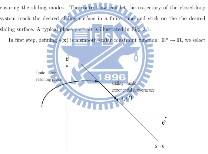
According to [37], the two-step procedure for sliding mode control design was clearly stated: 1) Sliding surface design. When the trajectory of closed-loop system is fixed in the sliding surface, it will be asymptotically stable. And, 2) Discontinuous controllers ensuring the sliding modes. The control law can let the trajectory of the closed-loop system reach the desired sliding surface in a finite time and stick on the the desired sliding surface. A typical phase portrait is illustrated in Fig. 2.1.

In first step, defining s(x) is a smooth scalar constraint function: IRn→ IR, we select

Fig. 2.1. A typical phase portrait under sliding mode control

time-varying sliding surface to be s = 0 with

where the constant coefficient vector aT _{= [a}

1 · · · ar]. Here, ai for i=1,· · · , r − 1 are

selected constants and ar = 1 is chosen such that

λr−1+ ar−1λr−2+· · · + a2λ + a1 (2.6)

are Hurwitz polynomials. As the states trajectory remain on the sliding surface, i.e., s = 0, we can know Eq. (2.5) will be asymptotically stable, which means the error approaches zero as the time approaches infinity.

Second, designing the control law u, consisting of two parts

u = ueq+ ure (2.7) where ueq is continuous called a feedback control law and ureis discontinuous or switched. As designing the ueq, there exists a condition which it must let the sliding surface s = 0 be invariant set relatively to the closed-loop system for unpresence of uncertainties or external disturbances of the matched type system [37]. That is s(x(t0)) = 0 and s(x(t)) = 0,

∀ t ≥ t0. Moreover, the time derivative of s is given by

˙s = aT˙e (2.8)

where

˙e = [ ˙e · · · e(r)]T (2.9) Expanding Eq. (2.8), the sliding variable dynamics as follows

˙s = f (x) + g(x)u + d(x)− x(r)_d

+ar−1e(r−1)+· · · + a2e + a¨ 1˙e (2.10)

Herein, it is regardless of d and ure such that u = ueq can verify sliding condition. The equilibrium point of Eq. (2.10) will be s = 0. ueq is designed as

ueq =− 1 g(x) [ f (x)− x(r)_d + ar−1e(r−1)+· · · + a2e + a¨ 1˙e ] (2.11)

The effect of ueq _{is to eliminate the known form of Eq. (2.10). Substituting designed u}eq

into Eq. (2.10), we get

Obviously, if we do not consider the disturbance term d and just use the feedback controller u = ueq, Eq. (2.12) exists a equilibrium point at s = 0. Next, we consider Eq. (2.12) and assume s(e(t0))̸= 0 to design ure. The action of ure is to make sliding variable s be zero

in a finite time. That is the trajectory of the closed-loop system will achieve the sliding surface in limited time. To guarantee the reaching condition, we impose a assumption:

Assumption 2.1 There exists a nonnegative number ρ(x) such that

|d(x)| ≤ ρ(x) (2.13)

From Eq. (2.12), we obtain the other controller ure designed as

ure =− 1 g(x)[ρ + η] sgn(s) (2.14) where sgn(s) :=    1 if s > 0 0 if s = 0 −1 if s < 0

is the sign function (2.15)

and η > 0 is selected positive constant. Then, we substitute Eq. (2.14) into Eq. (2.12), the sliding variable dynamics becomes

˙s = − [ρ + η] sgn(s) + d(x) (2.16) In order to prove the feasibility of Eq. (2.14), with V = 1/2s2 _{as a Lyapunov function}

candidate for Eq. (2.16), we have

˙

V = s ˙s =− [ρ + η] s · sgn(s) + s · d(x) (2.17) Using the relation of s· sgn(s) = |s| and Cauchy-Schwarz inequality to get s · d(x) ≤ |d(x)||s| and Assumption 2.1, the time derivative of Lyapunov function candidate becomes

˙

V = − [ρ + η] s · sgn(s) + s · d(x) ≤ − [ρ + η] |s| + |d(x)||s| ≤ − [ρ + η] |s| + ρ|s|

According to (2.18), we have known that the Lyapunov function converges. The result explains that the Eq. (2.16) is asymptotically stable, i.e., s → 0 as t → ∞. In other words, focusing on Eq. (2.12), ure will make s approach the sliding surface in limited time when the sliding variable is not zero. Now, we discuss when the sliding variable reach the sliding surface. Actually, there is another form of the time derivative of Lyapunov function presented as ˙ V = d dtV = 1 2 d dt|s| 2 _=|s| d dt|s| (2.19) As a result of Ieq. (2.18) and Eq. (2.19), we obtain

|s|d

dt|s| ≤ −η|s| (2.20) That is

d

dt|s| ≤ −η (2.21)

It implies that |s| converges along with its slope less than or equal to −η. Integrating Ieq. (2.21) with t on [0, tr], we get ∫ tr 0 d|s(x(t))| dt dt≤ − ∫ tr 0 ηdt (2.22) According to the second fundamental theorem of calculus [38], Eq. (2.22) equals

|s(x(t))| − |s(x(0))| ≤ −ηt (2.23) or

0≤ |s(x(t))| ≤ |s(x(0))| − ηt (2.24) The above inequality shows that |s(x(t))| must converge before t = |s(x(0))|/η, which is illustrated in Fig. 2.2.

However, in order to account for the presence of modelling uncertainties and distur-bances, the control law has to be discontinuous across s(t). Since the implementation of the associate control switchings is necessarily imperfect (for example, in practice switching is not instantaneous, and the value s is not known with infinite precision), this leads to

Fig. 2.2. Sliding condition

chattering which is shown as Fig. 2.3. Now, chattering is undesirable in practice, since it involves high control activity and further may excite high-frequency dynamics neglected in the course of modelling such as unmodeled structure modes, neglected time-delays, and so on. Thus, in a second part, the discontinuous control law ure _{is suitably smoothed}

to achieve an optimal trade-off between control bandwidth and tracking precision: while the first part accounts for parametric uncertainty, the second part achieves robustness to high-frequency unmodeled dynamics [20].

2.2

Terminal Sliding Mode Control (TSMC)

Although the CSMC has received much attention as an efficient control technique for handling systems with large uncertainties, nonlinearities, and bounded external distur-bances and can guarantee finite-time convergence to the sliding surface, the closed-loop system states may only be guaranteed within infinite time. Thus, the terminal sliding mode control (TSMC) was evolved by Zak in the Jet Propulsion Laboratory (JPL) in 1988 [39]. The main idea of TSMC is the concept of terminal attractors which guarantee finite time convergence of the states. The TSMC was first introduced to the control of the dynamic systems based on second-order differential equations. After that, Yu and Man [40], [41] extended it to high-order system (2.1). The problem formulation is the same as Section 2.1. Defining s(x)i for i=1,· · · , r − 1 is a smooth scalar constraint function:

IRn → IR, the hierarchical terminal sliding mode structure is s1 = ˙s0 + b1s q1/p1 0 (2.25) s2 = ˙s1 + b2s q2/p2 1 (2.26) .. . sr−1 = ˙sr−2+ br−1s qr−1/pr−1 r−2 (2.27)

where s0 = e, bi > 0, pi > qi and pi, qi are positive odd integers This assumption allows

us to achieve high-order continuous differentiation. For instance, the geometry plot for third-order system is shown in Fig. 2.4.

The control is divided into

u = ueq+ ure (2.28) where ueq _{is the equivalent control for system (2.1) without model uncertainties and}

external disturbances, such that sr−1 = 0 and ˙s = 0 and ure is to compensate the internal

parameter variations and turbulence. Furthermore, the time derivative of sr−1 is given by

d dtsr−1 = d2 dt2sr−2+ br−1 d dts qr−1/pr−1 r−2 (2.29)

Besides, it can be easily calculated that d2 dt2sr−2 = d3 dt3sr−3+ br−2 d2 dt2s qr−2/pr−2 r−3 (2.30) d3 dt3sr−3 = d4 dt4sr−4+ br−3 d3 dt3s qr−3/pr−3 r−4 (2.31) .. . (2.32) d(r−2) dt(r−2)s2 = d(r−1) dt(r−1)s1+ b2 d(r−2) dt(r−2)s q2/p2 1 (2.33) d(r−1) dt(r−1)s1 = d(r) dt(r)s0+ b1 d(r−1) dt(r−1)s q1/p1 0 (2.34)

Substituting Eqs. (2.52)-(2.34) into Eq. (2.29), we obtain d dtsr−1 = d(r) dt(r)s0+ r−2 ∑ k=0 bk+1 d(r−1−k) dt(r−1−k)s qk+1/pk+1 k (2.35)

Importing Eq. (3.4), the time derivative of sr−1 will be

˙sr−1 = f (x) + g(x)u + d(x)− xrd + r−2 ∑ k=0 bk+1 d(r−1−k) dt(r−1−k)s qk+1/pk+1 k (2.36)

Thus, the controller u is designed as follows:

ueq =− 1 g(x) [ f (x)− xr_d+ r−2 ∑ k=0 bk+1 d(r−1−k) dt(r−1−k)s qk+1/pk+1 k ] (2.37) and ure =− 1 g(x)[ρ + η] sgn(s) (2.38)

Since |d| ≤ ρ, s · sgn(s) = |s|, Cauchy-Schwarz inequality s · d(x) ≤ |d(x)||s|, and selected positive constant η which have been accounted for in Section 2.1., the resulting expression is substituted into Eq. (2.37) and Eq. (2.38) and multiplied by sr−1 as

sr−1˙sr−1 = − [ρ + η] s · sgn(s) + s · d(x)

≤ − [ρ + η] |s| + |s||d(x)| ≤ − [ρ + η] |s| + ρ|s|

≤ −η|s| (2.39)

which means that the sliding mode sr−1 = 0 will be reached in finite time along with

its slope less than or equal to −η proved in Section 2.1. The finite time is directly proportional to the initial norm of sr−1 and the selected positive constant η expressing as

tr ≤ |s(x(0))/η|. However, the magnitude of the designed controller will become infinity

if si = 0 when ˙si ̸= 0. That is, it is the singularity problem. For example, the controller

of second-order system is described

u =− 1 g(x) [ f (x)− x2_d+ b1(q1/p1) e(q1/p1)−1˙e + (ρ + η) sgn(s) ] (2.40)

The term b1(q1/p1) e(q1/p1)−1˙e will occur singularity phenomenon since e(q1/p1)−1 = 1/e((p1−q1)/p1

where (q1/p1)− 1 = (q1− p1)/p1 is negative constant causes 1/e(p1−q1)/p1 → ∞ as e → 0.

In this situation, if ˙e = 0, the designed controller diverges. The problem is unexpected and will be solved in later Section.

Next, we will discuss whether or not the closed-loop system states can converge within finite time when sliding condition is exactly verified. First, importing the second-order differential equations [42], basically a nonlinear switch line,

s = ˙e + beq/p (2.41) where e = x − xd, b > 0, p, q are positive odd integers and p > q. Similar to the

conventional sliding mode control technique, if the controller is designed such that s converges to zero, then we say that the switching variable s reaches the terminal sliding mode

It has been shown in Zak [39] that e = 0 is the terminal attractor of dynamics (2.42). For a error e(tr) at t = tr when s = 0, then we integrate the time derivative of ˙e =−beq/p to

predict the convergence time ts at the sliding regime. That is

∫ ts+tr tr −1 be −q/p_{de =} ∫ ts+tr tr dt (2.43) Then, we have −p b(p− q)e(tr+ ts) 1−q p + p b(p− q)e(tr) 1−q p _{= t} s (2.44)

According to the conditions: 1) p, q are positive odd integers; and 2) p > q, we multiply −b(p − q)/p into Eq. (2.44) and move the second term of left to the right

0≤ |e(tr+ ts)| 1−q p = −b(p− q) p ts+|e(tr)| 1−q p _(2.45) Obviously, as ts = p b(p− q)|e(tr)| 1−q p _(2.46) we can verify 0≤ |e(tr+ ts)| 1−q p ≤ 0 (2.47)

The expression (2.46) means that in terminal sliding mode (2.42) the state error e con-verges to zero in finite time, the same for ˙e. The total time reaching e = 0 is t = tr+ ts.

Then, expanding to high-order continuous differentiation. With the structure (2.26)-(2.27), if sr−1 = 0 is reached, the stability and finite-time reachability of system

equilib-rium will be guaranteed because it is a concatenation of r dynamics of Eq. (2.41) type. If sr−1 = 0 is reached at t = tr = ts0, then sr−2 will reach sr−2 = 0 at

ts1 = tr+ pr−1 br−1(pr−1− qr−1)|s r−2(tr)| 1−qr−1 pr−1 _(2.48)

The general form of the convergent time tsi for sr−1−i will reach sr−1−i = 0 for i=1,· · · ,

(r− 1) is described by

ts0 = tr (2.49)

and tsi = ts(i−1)+

pr−i

br−i(pr−i− qr−i)

sr−1−i(ts(i−1)) 1−qr−1

The total time reaching e = 0 is t = ts0+ r−1 ∑ i=1 p_r−i br−i(pr−i− qr−i)

sr−1−i(ts(i−1)) 1−qr−1

pr−1 _(2.51)

TSMC adds nonlinear functions into the design of the sliding upper plane. A ter-minal sliding surface is constructed and the tracking errors on the sliding surface converge to zero in a finite time. Thus, the TSMC can guarantee that the system will achieve the desired output in finite time if the controller is designed by Eqs. (2.37) and (2.38).

2.3

Nonsingular Terminal Sliding Mode Control (NTSMC)

The TSMC is characterized, like the CSMC, by strong robustness to uncertainties and disturbances and guaranteed to achieve the desired state in finite time, yet it exists a singular problem for control law, for instance in second-order system, if ˙e ̸= 0 when e = 0; that is, u → ±∞ if ˙e ̸= 0 as e = 0. In order to overcome the singularity problem in the conventional TSMC systems, several methods have been proposed. For instance, one approach is to switch the sliding mode between terminal sliding mode and linear hyperplane based sliding mode [43]. Another approach is to transfer the trajectory to a pre-specified open region where TSMC is not singular [41]. These methods are adopting indirect approaches to avoid the singularity. Thus, in 2001, Feng [44] proposed a novel TSMC for second-order system, called nonsingular terminal sliding mode control (NTSMC) to overcome the singularity problem. The time taken to reach the manifold from any initial state and the time taken to reach the equilibrium point in the sliding mode can be guaranteed to be finite time. However, the NTSMC is just adapted to the second-order system. In other words, selecting n = 2 for system (2.1). Choosing the sliding surface of the second-order NTSMC:

s = e +1 c˙e

p1/q1 _(2.52)

where c = bp1/q1

1 , and p1, q1 are positive odd integers under the constraint 1 < (p1/q1) < 2.

One can easily see that when s = 0, Eq. (2.52) is equivalent to Eq. (2.26) for n = 2 so that the time of convergence is the same as TSMC for n = 2 when s = 0. For convenience, we simplify p1, q1 as p, q, respectively. The finite time is taken to to travel from e(tr)̸= 0

at t = tr to e(tr+ ts) is given by ts = p b(p− q)|e(tr)| 1−q p _(2.53)

Note that in using Eq. (2.52) the derivative of s along the system dynamics does not result in terms with negative powers, but the parameters p and q must satisfy the constraint 1 < p/q < 2 in addition. Next, we will account for the derivation process of the NTSMC controller. The controller is chosen

u = ueq+ ure (2.54) where ueq _{is the feedback control for system (2.1) for n = 2 without model uncertainties}

and external disturbances, such that s = 0 and ˙s = 0 and ure_{is to compensate the internal}

parameter variations and turbulence. Furthermore, the time derivative of s is given by

˙s = ˙e + 1 c ( p q ) ˙e p q−1_{¨e (2.55)} Hence, the controller u can be designed as follows:

ueq=− 1 g(x)  f(x) − x2 d+ c ( q p ) ˙e 2− p q   (2.56) and ure =− 1 g(x)[ρ + η] sgn(s) (2.57) Since |d(x)| ≤ ρ, s · sgn(s) = |s|, Cauchy-Schwarz inequality s · d(x) ≤ |d(x)||s|, and selected positive constant η which have been accounted for in Section 2.1, the resulting expression of Eq. (2.55) is substituted into Eq. (2.56) and Eq. (2.57) and multiplied by s as s ˙s = s· { 1 c ( p q ) ˙e(p/q)−1[(ρ + η) sgn(s) + d(x)] } · ≤ 1 c ( p q ) ˙e(p/q)−1[− (ρ + η) |s| + |d(x)||s|] ≤ 1 c ( p q ) ˙e(p/q)−1[− (ρ + η) |s| + ρ|s|] ≤ −1 c ( p q ) ˙e(p/q)−1η|s| (2.58)

Because p and q are positive odd integers and 1 < p/q < 2, there is ˙e(p/q)−1 _{> 0 for ˙e}̸= 0. Let R( ˙e) = 1 c ( p q )

˙e(p/q)−1η. As a result, we know R( ˙e) > 0 for ˙e̸= 0. Eq. (2.58) can be modified as

s ˙s ≤ −R( ˙e)|s| for ˙e ̸= 0 (2.59) will the NTSMC s = 0 be reached within finite time? The answer is yes [45]. The condition for Lyapunov stability is satisfied for the case ˙e ̸= 0. According to Eq. (2.59), it implies that the slope of sliding variable is always negative expect for ˙e = 0. In addition, for the case ˙e = 0, substituting the control (2.56) and (2.57) into the second equation of (2.1) yields ¨ e = −cq p˙e 2−p q + d(x) − (ρ + η) sgn(s) (2.60) It can be easily seen that if ˙e = 0, then Eq. (2.60) becomes

¨

e = d(x)− (ρ + η) sgn(s) (2.61) which suggests that ˙e = 0 while e ̸= 0 is not an attractor. For the cases of s > 0 and s < 0, we can obtain ¨e ≤ −η and ¨e ≥ η, respectively. In detail, there exists a vicinity | ˙e| ≤ δe˙ for a small

δe˙= ( η 2 p cq ) q 2q− p (2.62)

For s > 0 and ˙e > 0, when ˙e(t) reaches δe˙ from an initial state error rate ˙e(0), we can

obtain ¨ e = −cq p˙e 2−p q + d(x) − (ρ + η) ≤ −cq p˙e 2−p q − η ≤ −η 2 (2.63) It means ˙e(t) is monotonous decreasing and at least at the speed of η

2 cross the vicinity δe˙ within the finite time

tδe˙ ≤

2 ( ˙e(0)− ˙e(tδe˙))

η =

4δe˙

η (2.64) In the same manner, for s < 0 and ˙e < 0, when ˙e(t) reaches δe˙ from an initial state error

rate ˙e(0), we can obtain

¨ e = −cq p˙e 2−p q + d(x) + (ρ + η) ≥ −cq p˙e 2−p q + η ≥ η 2 (2.65)

It means ˙e(t) is monotonous increasing and at least at the speed of η

2 cross the vicinity δe˙ within the finite time

tδe˙ ≤

2 ( ˙e(tδe˙)− ˙e(0))

η =

4δe˙

η (2.66) Therefore the crossing of trajectory from one boundary of the vicinity ˙e = δe˙ to the other

boundary ˙e = −δe˙ for s > 0 and from ˙e = −δe˙ to ˙e = δe˙ for s < 0 is finite time. For

the region outside the | ˙e| < δe˙, the time to reach the boundaries of the vicinity is finite.

Indeed, we can easily show that

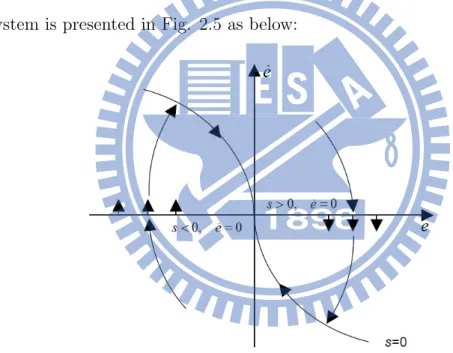
s ˙s ≤ −δR( ˙e)|s| (2.67) meaning the finite time reachability of the boundaries. The phase plane plot of the second-order system is presented in Fig. 2.5 as below:

Fig. 2.5. The phase plot of the second-order system

Therefore we can conclude that the switching line can be reached within finite time. Furthermore, the designed controller does not contain the singularity term to occur singu-larity phenomenon compared with TSMC because the term c (q/p) ˙e2−(p/q) _{of Eq. (2.56)}

does not yield singularity under the constraint 1 < (p/q) < 2. Thus, a NTSMC use the other nonlinear functions into the design of the sliding upper plane to not only over-come the singularity problem of TSMC but also verify the convergence of tracking desired output in finite time.

2.4

Mathematical Models of the Missile

2.4.1 Coordinate Systems

I) Definitions of Coordinate Frames

Before proceeding with the derivation, it is necessary to assume that the earth is an inertial reference, and unless otherwise stated the atmosphere is fixed with respect to the earth [46]. In addition, the coordinate systems adopted in the present discussion are right-handed axis systems.

i) Earth (Inertial) coordinate frame (Oxgygzg)

The origin Og is at the ground tracker. Oxg-axis is taken as north. The

positive Oyg-axis points upward in the vertical plane including Oxg-axis. The

positive Ozg-axis is the right direction or completes the right-handed coordinate

system.

ii) Body coordinate frame (Oxbybzb)

The origin Ob is at the center of gravity of the missile. The positive Oxb-axis

coincides with the center line (or longitudinal axis) of the missile or forward direction. The positive Oyb-axis points upward in the vertical plane including

Oxb-axis. The Ozb-axis completes the right-handed coordinate system.

iii) Ballistic coordinate frame (Oxtytzt)

The origin Ot is at the center of gravity of the missile. The positive Oxt-axis

coincides with the velocity of the missile. The positive Oyt-axis points upward in

the vertical plane including Oxt-axis and perpendicular to the horizontal plane

of the earth. The Ozt-axis completes the right-handed coordinate system.

iv) Wind coordinate frame (Oxvyvzv)

The origin Ov is at the center of gravity of the missile. The positive Oxv

-axis coincides with the velocity of the missile. The positive Oyv-axis points

upward in the vertical plane including Oxv-axis. The Ozv-axis completes the

right-handed coordinate system. Note that if the wind coordinate frame is nonrotating with respect to Oxv-axis and the initial definition of the Oyv-axis

of Oyv-axis is always the same as Oyt-axis), it is equal to ballistic coordinate

frame.

II) Definitions of Angles

Herein, in order to clearly understand the definitions of the angles, the plus or minus sign of each angle is according to a rule which the rotation axis directs to the reader.

i) Angles between wind frame and body frame

α: It is between Oxv-axis and the plane composed of Oxb-axis and Ozb-axis

and defined the sign is positive when Oxv-axis is under that plane.

β: It is between Oxv-axis and the plane composed of Oxb-axis and Oyb-axis

and defined the sign is positive when Oxv-axis is on the right of that plane.

Fig. 2.6. Definitions of α and β

ii) Angles between ballistic frame and wind frame

γv: It is between Ozv-axis and the plane composed of Oxt-axis and Oyt-axis

and defined the sign is positive when Ozv-axis is on the left of that plane.

iii) Angles between inertial frame and ballistic frame

θ: It is between Oxt-axis and the plane composed of Oxg-axis and Ozg-axis

and defined the sign is positive when Oxt-axis is on the above of that plane.

Fig. 2.7. Definition of γv

and defined the sign is positive when Oxt-axis is on the left of that plane.

Fig. 2.8. Definitions of θ and ψv

iv) Angles between inertial frame and body frame

ϑ: It is between Oxb-axis and the plane composed of Oxg-axis and Oyg-axis

and defined the sign is positive when Oxb-axis is on the above of that plane.

ψ: It is between Oxb-axis and the plane composed of Oxg-axis and Ozg-axis

and defined the sign is positive when Oxb-axis is on the left of that plane.

γ: It is between Oyb-axis and the plane composed of Ox′g-axis and Oyg-axis

and defined the sign is positive when Oyb-axis is on the left of that plane.

III) Coordinate Transformation

Define Mk(ϕ) to be the rotation by k axis with angle ϕ which any one frame is

Fig. 2.9. Definitions of ϑ, ψ, and γ

matrix (DCM). So far as the surface-to-air missile is concerned, each one coordinate follows three rotated steps to other one: 1) yaw, 2) pitch, and 3) roll, and the derivation of the transformation only is established in the direction presented in Fig. 2.10. The DCM rotated by the axes y, z, and x will be:

My(ϕ) =   c0ϕ 01 −s0ϕ sϕ 0 cϕ   Mz(ϕ) =   _−scϕ_ϕ scϕϕ 00 0 0 1   (2.68) Mx(ϕ) =   10 c0ϕ s0ϕ 0 −sϕ cϕ   where cϕ and sϕ denote cos ϕ and sin ϕ, respectively.

Fig. 2.10. The relationships among coordinates

i) Wind frame transforms to body frame T_vb(α, β) =   _−scα_α scαα 00 0 0 1     c0β 01 −s0β sβ 0 cβ   =   _−scα_αcβcβ csαα −csααssββ sβ 0 cβ   (2.69) ii) Ballistic frame transforms to wind frame

T_tv(γv) =   10 c0γv s0γv 0 −sγv cγv   (2.70) iii) Inertial frame transforms to ballistic frame

T_gt(θ, ψv) =   _−scθ_θ scθθ 00 0 0 1     c0ψv 01 −s0ψv sψv 0 cψv   =   _−scθc_θψcψvv scθθ −csθsθsψψvv sψv 0 cψv   (2.71) iv) Inertial frame transforms to body frame

T_gb(γ, ϑ, ψ) =   10 c0γ s0γ 0 −sγ cγ     _−scϑ_ϑ scϑϑ 00 0 0 1     c0ψ 01 −s0ψ sψ 0 cψ   =   _−sϑcψccϑγcψ+ sψsγ cϑscϑγ sϑsψ−ccγϑ+ csψψsγ sϑcψsγ+ sψcγ −cϑsγ −sϑsψsγ+ cψcγ   (2.72)

2.4.2 Rigid-Body Equations of Motion

In this section we will consider a typical missile and derive the equations of motion according to Newton’s laws. In deriving the rigid-body equations of motion, the following assumptions will be made [46], [47], [48]:

I) The missile is a rigid body, that is, the missile does not undergo any change in size and shape.

II) The missile is approximate a cylinder, that is, it is an axisymmetric or rotational symmetry missile.

III) The mass of the missile remains constant during any particular dynamic analysis.

IV) The aerodynamic forces and moments acting on the missile are invariant with the roll position of the missile relative to the free-stream velocity vector.

In addition, we note that in general, a vector Q can be transformed from a fixed frame OXY Z to a rotating coordinate system oxyz by the relation [49]

˙

QOXY Z = ˙QOxyz+ ωQ× Q (2.73)

where ωQ is the angular velocity of a rotating frame relatively to a fixed frame.

Further-more, if the rotating frame stops rotating, the two frames will has the same time rate of the change of state variables. Herein, the equations of motion are derived by the kine-matics and dynamics. They will be presented in four formats: I) kinekine-matics equations of translation about mass center, II) kinematics equations of rotation about mass center, III) dynamics equations of translation about mass center, and IV) dynamics equations of rotation about mass center, respectively [46], [47], [48].

I) Kinematics of Translation about Mass Center

In engineering practice, it is the simplest criterion for describing the missile trans-lation in the ballistic frame. Denoting the angular velocity of ballistic frame rela-tively to inertial frame by Ω and the missile velocity V, the missile velocity expressed in the ballistic frame can be written in the form

mdV dt = m ( δV δt + Ω× V ) (2.74)

Let us first resolve the vector Ω and V into components Ωtx, Ωty, Ωtz and Vtx, Vty,

Vtz, respectively, along the axes of the ballistic frame. Denoting by itx、jty、ktz

the corresponding to unit vectors of the ballistic frame (Oxtytzt), we write

Ω = Ωtxitx+ Ωtyjty+ Ωtzktz (2.75) V = Vtxitx+ Vtyjty+ Vtzktz (2.76) δV δt = dVtx dt itx+ dVty dt jty+ dVtz dt ktz (2.77)

where  VVtxty Vtz   =  V0 0   (2.78)

Substituting from Eq. (2.78)into Eq. (2.76)， δV

δt = dV

dt itx (2.79) The Eq. (2.74) will be

Ω× V =    ixt jzt kzt Ωxt Ωyt Ωzt V 0 0   = V Ωztjty− V Ωytktz (2.80)

And, we have known that

Ω = ˙ψv + ˙θ (2.81)

where ˙ψv and ˙θ are on the Ozg-axis and Oyt-axis, respectively. Eq. (2.81) can be

modified as   ΩΩxtyt Ωzt   =   _−scθ_θ scθθ 00 0 0 1     _ψ0˙ v 0   +   00 ˙ θ   =   ˙ ψvsθ ˙ ψvcθ ˙ θ   (2.82)

Replacing Eq. (2.80) with Eq. (2.82), we have

Ω× V =   V ˙0θ −V ˙ψvcos θ   (2.83)

Hence, substituting from Eqs. (2.77) and (2.79) into Eq. (2.74), we obtain    Ftx = m ˙V Fty = mV ˙θ Ftz =−mV ˙ψvcθ (2.84)

where Ftx, Fty, Ftz are the components of net external force, which is formed by

thrust, aerodynamic force, gravity, and lateral force, etc., with respect to the ballistic frame. Herein, we only analyze the first four sources of external force and the others are regarded as disturbances.

i) Thrust vector control (TVC)

The positive force of TVC Fpb is fixed in the direction of Oxb-axis; that is,

Fpb =   F0p 0   (2.85)

Using Eqs. (2.69) and (2.70), the force can be projected onto the ballistic frame and denoted as Fpt. Fpt = (Ttv) T( T_vb)T Fpb =   Fp(sαcFγvpc+ cαcβαsβsγv) Fp(sαsγv− cαsβcγv)   (2.86) ii) Aerodynamic force

The components of the force are defined as the positive drag force X along negative Oxv-axis, the lift force Y positive to the Oyb-axis, and the side force

positive to the Ozb-axis in the wind frame. Using Eq. (2.70), we can project it

onto the ballistic frame.  FFatxaty Fatz   = [Tv t] T   −XY Z   =   Y cγv−X− Zsγv Y sγv+ Zcγv   (2.87) iii) Lateral thrust force

The components of the force are in the directions of Oyb-axis and Ozb-axis

in the body frame, respectively. In the same manner as thrust vector force, we have [ Ftty Fttz ] = [ Ftby(cαcγv − sαsβsγv)− Ftbz(cβsγv) Ftby(cαsγv+ sαsβcγv) + Ftbz(cβcγv) ] (2.88)

iv) Gravity force

The negative force is in the direction of Oyg-axis. Using Eq. (2.71), the force

can be projected onto the ballistic frame.   mgmgtxty mgtz   = (Tt g )_ 0 −mg 0   =   −mgs_−mgcθ_θ 0   (2.89)

Substituting Eqs. (2.86)-(2.89) into Eq. (2.84), the kinematics equations of trans-lation about mass center are

                   ˙ V = 1 m(Fptx+ Fatx + mgtx) ˙ θ = 1

mV (Fpty + Faty+ Fltty + mgty) ˙

ψv = −1

mV cθ

(Fptz+ Fatz+ Flttz + mgtz)

(2.90)

II) Kinematics of Rotation about Mass Center

In engineering practice, it is the simplest criterion for describing the missile ro-tation in body frame. Denoting the angular velocity of body frame corresponding to inertial frame by ω and the angular momentum H, the kinematics equations of rotation about mass center has the form [49]

dH dt =

δH

δt + ω× H (2.91) The vectors ω and H are divided into components ωbx, ωby, ωbz and Hbx, Hby,

Hbz,respectively, along the axes of the body frame. Denoting by ibx, jby, kbz the

corresponding to unit vectors of the body frame, we write

ω = ωbxibx + ωbyjby + ωbzkbz (2.92)

H = Hbxibx+ Hbyjby + Hbzkbz (2.93)

The first term of the right side in Eq. (2.91) will be δH δt = dHbx dt ibx+ dHby dt jby+ dHbz dt kbz (2.94) Besides, we have known that

H = I· ω (2.95)

where I is inertia tensor, including moments and products of inertia. According to the assumption 2, the products of inertia are zero in the body frame and Eq. (2.95) can be simplified as follows

 HHbxby Hbz   =  IIxxyyωωbxby Izzωbz   (2.96)

Replacing the second term of the right side in Eq. (2.91) with Eq. (2.92) and Eq. (2.96), we can obtain ω× H =    ibx jby kbz ωbx ωby ωbz Ixxωbx Iyyωby Izzωbz   =   (I(Ixxzz− I− Iyyzz)ω)ωbybxωωbzbz (Iyy − Ixx)ωbxωby   (2.97) Substituting Eqs. (2.94) and (2.97) into Eq. (2.91), we write

                 Mbx = Ixx ωbx dt + (Izz − Iyy)ωbyωbz Mby = Iyy ωby dt + (Ixx− Izz)ωbxωbz Mbz = Izz ωbz dt + (Iyy− Ixx)ωbxωby (2.98)

where Mbx, Mby, Mbz, which are the rolling, yawing, and pitching moments,

respec-tively, are the components of net external moment produced mainly by aerodynamic and lateral moments with respect to the body frame. Finally, we adjust Eq. (2.98), the kinematics equations of rotation about mass center are

                     ˙ ωbx= 1 Ixx [Mbx+ (Iyy− Izz)ωbyωbz] ˙ ωby = 1 Iyy [Mby+ (Izz − Ixx)ωbxωbz] ˙ ωbz = 1 Izz [Mbz + (Ixx− Iyy)ωbxωby] (2.99)

III) Dynamics of Translation about Mass Center

These equations are defined in the inertial frame such that we will understand the trajectory of the missile clearly. Furthermore, we must consider the altitude of the missile when calculating air density, dynamic pressure, and aerodynamic force. Hence, it is necessary to build these equations. In order to get these vectors, we must use Eqs. (2.69) and (2.72) to let Eq. (2.78) project into the inertial frame. The procedure is   y˙x˙ ˙z   = (Tb g )T( T_vb)   V0 0   (2.100)

Expanding the above equation, we have dynamics equations of translation about mass center as follows:

           ˙x = V [cαcβcϑcψ + sαcβ(sϑcψcγ− sψsγ) + sβsϑcψsγ+ sψcγ)] ˙ y = V (cαcβsϑ− sαcβcϑcγ− sβcϑsγ) ˙z =−V [cαcβcϑsψ+ sαcβ(sϑsψcγ+ cψsγ) + sβ(sϑsψsγ− cψcγ)] (2.101)

IV) Dynamics of Rotation about Mass Center

For the purpose of describing the attitude of the missile in the inertial frame, it is indispensable to construct these equations. According to the relationship between body frame and inertial frame, we have known

ω = ˙ψ + ˙ϑ + ˙γ (2.102)

where ˙ψ, ˙ϑ, and ˙γ are in the direction of Oyg-axis, Oz ′

g-axis, and Oxb-axis. We

can modify Eq. (2.102)on the basis of the regulation of coordinate transformation in this thesis.   ωωbxby ωbz   =   10 c0γ s0γ 0 −sγ cγ     _−scϑ_ϑ scϑϑ 00 0 0 1     _ψ0˙ 0   +   10 c0γ s0γ 0 −sγ cγ     00 ˙ ϑ   +   0˙γ 0   =   10 csϑϑcγ s0γ 0 −cϑsγ cγ     _ψ˙γ˙ ˙ ϑ   (2.103) Inversing the above matrix and expanding Eq. (2.103), the dynamics equations of rotation about mass center will be

                 ˙γ = ωbx− sϑ cϑ (ωbycγ− ωbzsγ) ˙ ψ = ωbycγ 1 cϑ − ωzbsγ 1 cϑ ˙ ϑ = ωbysγ+ ωbzcγ (2.104)

2.4.3 Equations of Attitude Dynamics

In guidance law design, inputs are the overloadings of the missle, while the autopilot must provide these overloadings to guidance law to successfully hit-to-kill the target.

Besides, the overloading is produced by angle of attack or sideslip angle. Herein, for convenience, we will build the equations of attitude of these two angles in the wind frame. The angular velocity in the wind frame can be separated into two parts: 1) one is yielded by wind frame relatively to body frame; 2) the other is yielded by body frame relatively to inertial frame and projected into the wind frame. That is,

ωv = (ωvb)v+ (ωbg)v (2.105) where (ωb_g)v = ( T_vb)T   ωωbxby ωbz   =   ωωbxbxcsααc+ ωβ − ωbycbyαsαcβ + ωbzsβ −ωbxcαsβ + ωbysαsβ+ ωbzcβ   (2.106) and (ωv_b)v =   _{− ˙β}0 0   +   c−β0 01 −s0−β s_−β 0 c_−β     00 − ˙α   =   αs_{− ˙β}˙ β − ˙αcβ   (2.107)

Then, we import Eq. (2.73) to express the acceleration of wind coordinate system relative to inertial coordinate system:

dV dt = ( δV δt + ωv× V ) (2.108) where δV δt =   ˙ V 0 0   (2.109) and ωv× V = (ωbg)v× V + (ωvb)v× V =    ivx jvy kvz ωb_{g vx} ω_{g vy}b ω_{g vz}b V 0 0   +    ivx jvy kvz ωv_{b vx} ω_{b vy}v ω_{b vz}v V 0 0    =   (−ωbxcαsβ + ωby0sαsβ+ ωbzcβ)V −(ωbxsα+ ωbycα)V   +   − ˙αc0βV ˙ βV   (2.110)