應用於液晶顯示器之薄型光致激發平面光源模組開發

國立交通大學

光電工程研究所

碩士論文

應用於液晶顯示器之

薄型光致激發平面光源模組開發

Development of Thin Format Light-Excited Flat

Lighting Systems for LCD Applications

研究生: 蕭博文

指導教授: 黃乙白 助理教授

田仲豪 副教授

應用於液晶顯示器之

薄型光致激發平面光源模組開發

Development of Thin Format Light-Excited Flat

Lighting Systems for LCD Applications

研究生： 蕭博文

Student: Bo-Wen Xiao

指導教授： 黃乙白

Advisor: Dr. Yi-Pai Huang

田仲豪

Dr. Chung-Hao Tien

國立交通大學 電機學院

光電工程研究所

碩士論文

A Thesis

Submitted to Institute of Electro-Optical Engineering

College of Electrical and Computer Engineering

National Chiao Tung University

in Partial Fulfillment of the Requirements

for the Degree of Master

in

Electro-Optical Engineering

June 2009

Hsinchu, Taiwan,

Republic of China

中華民國 九十八 年 六 月

i

應用於液晶顯示器之

薄型光致激發平面光源模組開發

碩士研究生：蕭博文

指導教授 黃乙白 助理教授

田仲豪 副教授

國立交通大學 光電工程研究所

摘 要

薄型化液晶電視（Slim format LCD-TV）逐漸成為顯示器市場趨勢。然而，在模組 厚度減低時，傳統背光系統面臨均勻度不佳等問題。設計高均勻度的超薄型背光系統成 為 液 晶 電 視 薄 型 化 關 鍵 所 在 。 本 論 文 應 用 外 層 螢 光 發 光 技 術 （ External Photo-fluorescent Technology），提出兩種應用於大尺寸直下式背光系統的光致激發

平面光源模組：紫外光激發式平面光源模組（UV Excited Flat Lighting System, UFL），

以及藍光激發式平面光源模組（Blue-Light Excited Flat Lighting System, BFL）。 然而，這種平面光源模組卻面臨了複雜的波長轉換機制，無法在模組硬體建立前先藉由 光學模擬軟體對系統結構優化。為了解決這個問題，本論文提出一套可信賴的波長轉換 機制光學模擬模型，成功地詮釋 UFL 模組以及 BFL 模組當中的光學特性。進一步藉由此 光學模型，針對 BFL 背光模組設計凸透鏡薄膜（Lenticular Film）提高正向視角亮度， 並改善側向視角色偏現象。藉由模擬和實驗結果，UFL 以及 BFL 背光模組成功地在超薄 厚度下展現高均勻度表現；使用凸透鏡薄膜也成功地提昇 BFL 背光模組正向亮度，同時 減少大角度色偏移。

：

ii

Development of Thin Format Light-Excited Flat Lighting Systems

for LCD Applications

Master Student: Bo-Wen Xiao

Advisor Dr. Yi-Pai Huang

Dr. Chung-Hao Tien

Institute of Electro-Optical Engineering

National Chiao Tung University

Abstract

Slim-format LCD-TV had been a trend for the current display market. However, conventional backlight systems suffered from insufficient uniformity when module thickness decreased. Designing ultra-slim-format backlight systems with high uniformity was the key factor to develop slim-format LCD-TVs. Basing on the External Photo-fluorescent Technology, this thesis proposed two light-excited flat lighting systems, the UV Excited Flat Lighting (UFL) System and the Blue-Light Excited Flat Lighting (BFL) System, for large-sized direct-emitting type backlight units. However, these proposed systems encountered complex wavelength-converting mechanisms and lacked of suitable simulation models for optimizing before manufacturing in practical. To solve this issue, an available wavelength-converting simulation model was proposed in this thesis. By this simulation model, the optical properties in the UFL and BFL systems were successfully analyzed. Furthermore, a lenticular film was designed for enhancing on-axis luminance and suppressing off-axis color deviation in the BFL system. By simulation and experimental results, the UFL and BFL systems successfully exhibited high uniform output with slim module thickness. Moreover, by embedding the lenticular film in the BFL system, the on-axis luminance was increased and the off-axis color deviation was suppressed effectively.

iii

誌謝

能夠順利完成本篇論文，首先要感謝黃乙白教授以及田仲豪教授。這兩年來，因為 有兩位指導教授的教導與啟發，讓我在學習研究上獲益良多，更從兩位教授身上學習到 正確待人處事的方法，在此致上最誠摯的謝意。 也很感謝仁宇學長，均合學長，健翔學長以及仁杰學長，在這兩年提供許多寶貴的 意見，不僅引導我在研究上突破瓶頸，更令我從挫折當中學習到該有的學習態度。另外， 要謝謝同樣身為背光組的靖堯，浩彣，以及姚順，在研究上給我許多的鼓舞支持，也在 閒暇之餘帶給我許多歡樂。兩年來建立的默契相信大家不會忘記。 此外，也很感謝宜伶，宗緯，俊賢，佑禎，拓江，高銘，宜如，以及益興，和你們 這些夥伴一起奮鬥的日子，是我一輩子珍惜的回憶。也很謝謝實驗室的學長姐以及學弟 妹們，有你們的陪伴，替兩年的碩士生涯添增樂趣。 最後，要謝謝我的家人，因為有你們的支持與付出，也因為有你們的教導，我才能 夠順利完成碩士學業。謝謝我家人對我付出的一切，謹以本文獻給家人和關懷我的人。

iv

Table of Contents

Abstract (Chinese) ... i

Abstract (English) ... ii

Acknowledge ... iii

Table of Contents ... iv

Figure Captions ... vi

List of Tables ... ix

Chapter 1 Introducation ... 1

1.1 Liquid crystal displays (LCDs) ... 1

1.2 Direct-emitting backlight systems ... 2

1.3 External photo-fluorescent technology ... 4

1.4 Motivation and Objectives ... 6

1.5 Organization of this Thesis ... 8

Chapter 2 Principle of Backlight System ... 9

2.1 Principles of ray-tracing method... 9

2.2 Radiometric and Photometric quantities ... 12

2.3 Bidirectional transmission and reflection distribution function ... 16

2.4 Colorimetry ... 18

2.5 Summary ... 22

Chapter 3 BTDF and BRDF Measurement Instrument ... 24

3.1 Conoscopic system ... 24

3.2 BTDF measurement system ... 26

3.3 Summary ... 28

Chapter 4 UV Excited Flat Lighting (UFL) System ... 29

v

4.2 Simulation model of UFL system ... 30

4.3 BTDF and BRDF measurement results ... 32

4.4 Simulation and experimental results ... 35

4.4.1 Simulation and optimization results ... 35

4.4.2 Simulation model verification ... 38

4.4.3 Experimental results of optimized UFL module ... 39

4.5 Dual-sided UFL System ... 41

4.6 Summary and discussion ... 42

Chapter 5 Blue-Light Excited Flat Light (BFL) System ... 44

5.1 The Light-emitting Mechanism of the BFL System ... 44

5.2 Simulation model of BFL system ... 46

5.3 BTDF and BRDF measurement results ... 47

5.4 Simulation results of the BFL system ... 51

5.4.1 Uniformity versus LED pitch and module gap ... 51

5.4.2 Angular color deviation versus LED pitch ... 53

5.4.3 Lenticular films and angular color deviation ... 56

5.5 Experimental results of the BFL system ... 60

5.6 Summary and discussion ... 65

Chapter 6 Conclusions and Future Work... 66

6.1 Conclusion ... 66

6.2 Future Work ... 67

vi

Figure Captions

Fig. 1-1 Schematic configuration of a liquid crystal display. ... 2

Fig. 1-2 Schematic configuration of the conventional direct-emitting backlight systems. ... 3

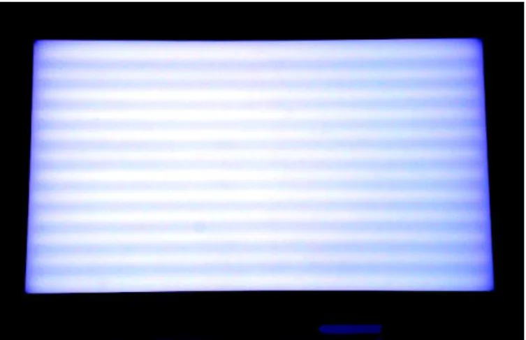
Fig. 1-3 Lamp-Mura defect of a 32-inch direct-emitting CCFL backlight systems captured by a charge-coupled device (CCD). ... 4

Fig. 1-4 Schematic configurations of light emitting diodes. ... 5

Fig. 1-5 Schematic configuration of (a) UV Excited Flat Lighting (UFL) system and (b) Blue-Light Excited Flat Lighting (BFL) system.. ... 7

Fig. 2-1 Defining geometry of radiometric quantities. ... 14

Fig. 2-2 Human visual response function. ... 16

Fig. 2-3 Schematic diagram of BTDF and BRDF. ... 17

Fig. 2-4 Color matching functions x( ) , y( ) , and z( ) in the CIE XYZ color system. .. 19

Fig. 2-5 xy chromaticity diagram of CIE XYZ color system. ... 20

Fig. 2-6 u’v’ chromaticity diagram of the CIELUV color system. ... 22

Fig. 3-1 Schematic of the conoscopic system in transmissive mode. ... 25

Fig. 3-2 Schematic of the conoscopic system in reflective mode. ... 26

Fig. 3-4 Diagram of BTDF measurement. ... 27

Fig. 3-3 Schematic of designed device for BTDF measurement. ... 27

Fig. 4-1 (a) Scheme of UFL system; (b) Cross-structure of UFL with relative modeling steps. ... 30

Fig. 4-2 Top view of the phosphor layer captured by a scanning electron microscope (SEM). ... 30

Fig. 4-3 Flowchart of modeling process of UFL system ... 31

Fig. 4-4 Schematic BTDF measuring process in a unit-lamp UFL module. ... 32

Fig. 4-5 Measured BTDFs (luminance in normal direction) of phosphor film for UV-to-visible light. ... 33

Fig. 4-6 Measured BTDFs (normalized angular distribution) of phosphor film for UV-to-visible light at 0-mm and 12-mm position with 10-mm height. ... 33

Fig. 4-7 Measured BTDF of (a) phosphor film and BRDFs of (b) phosphor film and (c) reflector, for visible-to-visible light. ... 34

Fig. 4-8 The configuration of the 4-lamps UFL system in simulated environment. ... 35

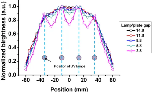
Fig. 4-9 The normalized on-axis luminance of the simulated 4-lamps UFL system (with different lamp/plate gap values). ... 37

vii

Fig. 4-10 The uniformity of the simulated 4-lamps UFL system (with different lamp/plate gap

values). ... 37

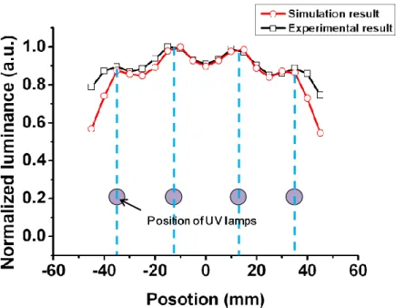
Fig. 4-11 Simulated and experimental on-axis luminance results of the 4-lamps UFL system. (with lamp/plate gap=5.8mm and lamp/lamp pitch=24mm) ... 39

Fig. 4-12 Lamp mura comparison between two backlight systems with slim-format design. . 40

Fig. 4-13 Measured luminance distribution of the UFL and CCFL systems (with diffuser plate) at 5.8mm lamp/plate gap. ... 40

Fig. 4-14 The 42-inch Dual-sided UFL system. ... 41

Fig. 4-15 Luminance comparison between dual-sided UFL and CCFL systems. ... 42

Fig. 4-16 Measured and the fitting curve of UV light intensity. ... 43

Fig. 5-1 (a) Configuration of the BFL system; (b) Cross-structure of the BFL system with light-emitting mechainsim. ... 45

Fig. 5-2 Flowchart of modeling process of the BFL system. ... 47

Fig. 5-3 Measured BTDFs of YAG-phosphor for (a) transmitted blue-to-blue light and (b) excited blue-to-yellow light. ... 49

Fig. 5-4 Measured BRDFs of YAG-phosphor for reflected blue-to-blue light. ... 49

Fig. 5-5 Measured (a) BTDF and (b)BRDF of the YAG-phosphor layer for transmitted and reflected yellow-to-yellow lights. ... 50

Fig. 5-6 Setup of the BFL system in the simulated environment. ... 52

Fig. 5-7 Uniformity with varied pitches and gaps for (a) the BFL system and (b) the conventional LED backlight (with 80% haze diffuser only). ... 53

Fig. 5-8 Uniformity comparison between the BFL system and the LED backlight system (with 80% haze diffuser alone) with 8-mm, 10-mm, and 12-mm module gaps. ... 53

Fig. 5-9 Setup of the BFL system in the simulated environment. ... 54

Fig. 5-10 The u’v’ chromaticity diagram of the BFL system with (a) 10-mm module gap and 10-mm LED pitch and (b) 10-mm module gap and 20-mm LED pitch. ... 55

Fig. 5-11 The color difference value (u’v’) of the BFL system with a fixed module gap (10mm) and varied LED pitches (4-20mm). ... 55

Fig. 5-12 Scheme of (a) the lenticular film and (b) the BFL system with double-crossed lenticular film. ... 57

Fig. 5-13 The color difference u’v’ in off-axis viewing direcitons of the double-crossed lenticular film adopted BFL system. ... 58 Fig. 5-14 Theu’v’ chromaticity diagram of the BFL system (a) without double-crossed

viii

lenticular film and (b) adopted with the double-crossed lenticular film (AR=0.4). 59 Fig. 5-15 The luminance in on-axis viewing direciton of the double-crossed lenticular film

adopted BFL system. ... 59 Fig. 5-16 The demonstrated 7-inch BFL system. ... 60 Fig. 5-17 The top view of the double-crossed lenticular film captured by a charge-coupled

device. ... 60 Fig. 5-18 The images captured by a charge-coupled device of the BFL system and the

diffuser-combined LED module. ... 62 Fig. 5-19 The measured uniformityies of the BFL system and the diffuser-combined LED

module. ... 62 Fig. 5-20 The u’v’ chromaticity diagram of the BFL system (a) without double-crossed

lenticular film and (b) adopted with the double-crossed lenticular film. ... 64 Fig. 5-21 The color difference values u’v’ in off-axis viewing direcitons of the BFL system.

... 64 Fig. 6-1 Light distributions of the BFL system with blue LED chips illuminating in different

numbers, ... 68 Fig. 6-2 Schematic configuration of the Fresnel lens embedded BFL system. ... 69

ix

List of Tables

Table 2-1 Radiometric units. ... 12

Table 2-2 Photometric quantities. ... 15

Table 2-3 Function of applied principles. ... 23

Table 4-1 Specification of the 4-lamps UFL system in simulated environment. ... 36

Table 4-2 Correlation coefficients between simulation and experimental results... 39

Table 5-1 Measured BTDFs and BRDFs of the YAG-phosphor layer. ... 48

Table 5-2 Specification of the BFL system and the double-crossed lenticular film. ... 61

1

Chapter 1

Introduction

Slim format LCDs had been a trend in the current display market. For producing a bright display image in large-sized LCD-TVs, direct-emitting backlight systems are used to provide sufficient brightness and uniform luminosity for the LC layer. However, the slim profile design of conventional direct-emitting backlights suffers from inadequate uniformity and the Mura defects. In this thesis, two novel light-excited backlight systems, the UV Excited Flat Lighting (UFL)[1] system and the Blue-Light Excited Flat Lighting (BFL)[2,3,4] system, are proposed. Both of them are based on the external photo-fluorescent technology and have the potential for fabricating slim format backlight unit for large-sized LCD applications.

1.1 Liquid crystal displays (LCDs)

In liquid crystal displays (LCDs), the liquid crystal (LC) acts as an electro-optic shutter which modulates the amount of incident light. Typical LCD configuration is shown in Fig.1-1 and consists of glass substrates, the LC layer, transparent electrodes, thin film transistors (TFTs), color filters, and polarizers[5]. The LC layer is placed between two glass substrates (e.g. indium tin oxide, ITO) and driven by a TFT to modulate the light transmission in each pixel of the LCD. The RGB color filter array is fabricated on the top glass substrate to mix the three monochromatic primary colors and produce full color images. The backlight system is assembled behind the LC panel to provide a uniform light source for the LCD because the LC modulates light only.

2

Fig. 1-1 Schematic configuration of a liquid crystal display.

In generally, the backlight system can be classified into two types depending on the position of the light source (e.g. cold cathode fluorescent lamp (CCFL)). The light source at the edge of, and directly behind, the LCD is called side-emitting and direct-emitting backlights, respectively. A side-emitting backlight is typically used in small and middle-sized LCDs because of its small form factor and low power consumption. However, large-sized LCDs, such as LCD-TVs, have a large display area, thus an increased light source is needed to achieve the specified brightness. Because side-emitting backlights are limited in increasing the light source, direct-emitting backlights are generally applied to large-sized LCDs.

1.2 Direct-emitting backlight systems

The conventional direct-emitting backlight systems consist of a diffusive plate, optical films, and light sources, as shown in Fig. 1-2[6]. The light sources, which are CCFL lamps or LEDs, are arranged parallel to the LC panel. A diffusive plate with diffusive particles inside the substrate is laid at a distance from the light source. When light is emitted from the light source, it is diffused by the diffusive plate and reflected by the reflector. Then, a bottom diffusive sheet, with adjusted scattering ability, is applied to obtain a more uniform light distribution. A prism sheet is then used to redirect the light from a large inclined angle in the normal direction[7]. Thus brightness can be enhanced in the normal viewing direction. Finally,

3

a top diffusive sheet, placed on top of the backlight system, is applied to protect the micro-structure of the prism sheet and to reduce Moiré patterns [8].

(a) CCFL backlight (b) LED backlight Fig. 1-2 Schematic configuration of the conventional direct-emitting backlight systems.

Such conventional configuration had already met a bottleneck in satisfying the requirements of slim format displays: slim, bright, and economic production simultaneously. The slim profile design causes low uniformity and induces Lamp-Mura defect[9] in the CCFL backlight, which used linear-source-like CCFLs as a light source, and Spot-Mura defect[10] in the LED backlight, which applied point-source-like LEDs to emit light rays, as shown in Fig.1-3. Currently, to improve Mura defects, there are straightforward methods that have been summarized by Schiavon[11]: 1) enlarging the gap between light sources and diffusive films. 2) multiplying the amount of diffusive films, and 3) increasing the number of light sources. However, the enlarged gap induces heavy system volume. Moreover, the multiplied amount of diffusive films and the increased light source number results in low optical efficiency and high cost. None of the methods mentioned above are adequate to the future slim format displays. Therefore, developing backlight systems which emit light rays directly from a flat surface as a planar light source is the oncoming objective.

4

Fig. 1-3 Lamp-Mura defect of a 32-inch direct-emitting CCFL backlight systems captured by a charge-coupled device (CCD).

1.3 External photo-fluorescent technology

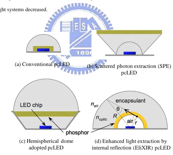
External photo-fluorescent technology was firstly developed for LED packaging since Nadarajah‟s research (2005)[12]

. A light-excited illuminating device configuring with remote phosphor structure is so-called external photo-fluorescent technology. Fig. 1-4(a) shows the scheme of the conventional pcLED which utilizes a blue LED chip irradiating Cerium(III)-doped Y3Al5O12 phosphor[13] (YAG-phosphor) to obtain white light emission. The broadband YAG-phosphor is coated on the LED die surface and packaged inside the device. This configuration has low efficiency because the diffuse phosphor directs 60% of total white light emission back toward the chip and leads losses of energy. Nadarajah et al. proposed the scattered photon extraction (SPE) pcLED[12] which contained a remote YAG-phosphor. The remote phosphor was coated outside the LED chips as shown in Fig. 1-4(b). Due to the separation of LED die and extraction of backward-emitted rays, the efficiency of SPE pcLED was 61% higher than conventional pcLED. Besides the SPE pcLED proposed by Nadarajah, the pcLED configuration of Fig. 1-4(c) introduced by Luo et al. (2005) utilized a remote phosphor, reflector cup, and hemispherical dome to minimize amount of trapped light[14]. In addition, Allen et al. (2008) proposed the enhanced light extraction by internal reflection (EliXIR) pcLED[15,16] which utilized a semitransparent phosphor that is

5

separated from the chip by an air gap, as shown in Fig.1-4(d). The semitransparent phosphor allows light to pass without deflection and escape device more easily. Beside, internal reflection at phosphor/air interface redirects much of the backward phosphor emission away from the die and reflective surface without loss.

The external photo-fluorescent technology adopted pcLEDs utilize blue LED chips to excite a remote phosphor for white light illumination. By separating phosphor from LED chips, these phosphor separated pcLEDs[12,14,15,16] obtained greater extraction efficiency and performed higher illuminating brightness when compared with conventional pcLEDs. However, these pcLEDs were not adequate to slim format backlight units. These pcLEDs were still point-source-like LEDs and caused spot-mura defect when module thickness of backlight systems decreased.

Fig. 1-4 Schematic configurations of light emitting diodes.

(a) Conventional pcLED _{(b) Scattered photon extraction (SPE)}

pcLED

(c) Hemispherical dome adopted pcLED

(d) Enhanced light extraction by internal reflection (EliXIR) pcLED

6

1.4 Motivation and Objectives

Slim format LCD-TVs had been a trend in the display market. However, the traditional direct-emitting backlight unit‟s uniformity has reduced while module thickness has decreased. A backlight unit with insufficient uniformity suffers from Mura defect and causes a low quality image. In order to evolve slim format LCD-TVs which can be mounted on a wall to save room space, the key factor is to develop backlight systems emitting planar light in slim profile directly.

Basing on research of the external photo-fluorescent technology adopted pcLEDs, the UV Excited Flat Lighting (UFL) [1] system and the Blue-Light Excited Flat Lighting (BFL) [2,3,4] system are proposed in this thesis. These two light-excited flat lighting systems are both based on the external photo-fluorescent technology and configure with large-sized remote phosphor layers coated on flat substrates, as shown in Fig.1-5. The UFL system differs from traditional CCFL backlights and consists of UV lamps placed inside the backlight cavity and phosphor layers coated on the top substrate and the bottom reflector. The BFL system differs from conventional LED backlights and consists of blue LED chips located on the bottom reflector and YAG-phosphor layer coated on the top substrate. For incident light will be redistributed on the flat remote phosphor layer, the UFL system and the BFL system could emit white light from the separated large-sized substrate directly. In other words, the UFL system and the BFL system could convert the linear sources (UV Lamps) or the point sources (blue LEDs) into a planar light source. Therefore, the UFL system and the BFL system have the potential for fabricating ultra-slim-format backlight systems for large-sized LCD-TV applications.

7

(a)

(b)

Fig. 1-5 Schematic configuration of (a) UV Excited Flat Lighting (UFL) system and (b) Blue-Light Excited Flat Lighting (BFL) system..

Creating an optical simulation model is essential for designing optimal structures of the UFL system and the BFL system. However, the optical phenomena of UFL and BFL systems are quite different from the traditional CCFL and LED backlight units. The optical properties which include simultaneously wavelength-converting mechanism and light-scattering mechanism of the remote phosphor films makes such backlight systems difficult to be simulated in commercial software. At present, there are no suitable simulation models that can describe such optical properties. Therefore, in this thesis, a reliable simulation model is

Reflector Bottom Phosphor UV Lamps PET Plate Top Phosphor x y YAG Phosphor PET Plate Reflector

Blue LED chips

x y

8

proposed to analyze the specific optical phenomena and optimize the geometrical structure of the UFL and BFL systems. We expect that the total module thickness of UFL system could be reduced to 15mm and that of BFL system could be further reduces to 10mm with over 80% uniformity. Additionally, by the developed simulation model, a lenticulr optical film is designed for enhancing on-axis luminance and suppressing off-axis color deviation of the BFL system.

1.5 Organization of this Thesis

The thesis is organized as follows: The principles of backlight systems are presented in

Chapter 2. In Chapter 3, the major instruments for characterizing backlight systems are

described. The modeling process of the UFL system is described and then the simulation results and the experimental results are verified in Chapter 4. The BFL system model and the experimental results are presented in Chapter 5. Finally, conclusions of this thesis and recommendations for the future work are presented in Chapter 6.

9

Chapter 2

Principles of Backlight System

For analyzing and designing backlight systems, some optical principles, radiometry, photometry, bidirectional transmittance and reflectance distribution function (BTDF and BRDF), and colorimetry, are described in this chapter. The ray-tracing method simplified behavior of light propagation. However, the optical characterizations of phosphor films, which included light-scattering mechanism and wavelength-converting mechanism simultaneously, were difficult to be described by ray-tracing only. Accordingly, the BTDF and BRDF based on radiometry and photometry are described and utilized to characterize the scattering characterization of phosphor film. Moreover, basing on colorimetry, the CIEXYZ and CIELUV color spaces, which specify color numerically, are also presented in this chapter.

2.1 Principles of ray-tracing method

Ray-tracing method is based on Snell‟s law, Fresnel‟s equation, and other optical principles. By electromagnetic theory, light is a kind of electromagnetic waves with time varying electric and magnetic fields. The light waves take a spherical form when just radiated from a point source and then behave like plane waves as traveling away the source. The path of a hypothetical point on the wave front of light is called a ray of light. Such a light ray is an extremely convenient fiction. Thus, the ray-tracing provides a simplified solution for discussing the behavior of light and analyzing optical systems. Therefore, some optical software, such as LightToolsTM, OSLOTM, et al., apply the ray-tracing method to build optical module for a simulated environment.

10

Snell’s law (Law of refraction)

Snell‟s law, also known as law of refraction, defines the appearance of refraction in the plane of incidence. A light ray making an angle i (the incidence angle) with the surface

normal strikes a boundary separating two optical media will induce a refracted ray transmitted through the boundary and makes a new angle t (the refraction angle) with the surface normal.

Snell‟s law says that the ratio of the incidence angle to the refraction angle of light equals to a constant which depends on the opposite ratio of the refractive indices of two optical media as[17]: sin sin i t t i n n    (2-1)

where ni and nt are the refractive indices of the incident and transmitting medium,

respectively.

Law of reflection

In the plane of incidence, the deviation of optical rays due to reflection is defined as the following equation, which is the so-called law of reflection[18]:

i r

  (2-2)

where i (incident angle) and r (reflected angle) are the angles made by the incident and

refracted ray with the surface normal, respectively. In other words, the reflected ray makes equal but opposite angle with the incident ray.

Fresnel’s equations

Fresnel‟s equations describe the energy of transmitted and reflected light at an interface between two different optical media. For the P (parallel to the plane of incidence) and S (perpendicular to the plane of incidence) polarization waves, the amplitude reflection and transmission coefficients r and t are respectively given by[19]:

11 cos cos cos cos i i t t s i i t t n n r n n        (2-3) 2 cos cos cos i i s i i t t n t n n      (2-4) cos cos cos cos t i i t p i t t i n n r n n        (2-5) 2 cos cos cos i i p i t t i n t n n      (2-6)

where ni and nt are the refractive indices of the incident and transmitting medium, i and t are

the angle of incidence and angle of propagation respectively.

According to irradiance[20], the reflectance and the transmittance for polarized light are defined as: 2 s s R r (2-7) 1 s s T  R (2-8) 2 p p R r (2-9) 1 p p T  R (2-10)

where Rs and Rp are the reflectances for S and P polarization light, and Ts and Tp are the

transmittances for S and P polarization light, respectively. When a random polarized light (eg. the nature light) strikes the interface, the reflectance R and transmittance T are defined as the average of the polarized case as following equations:

2 s p R R R  (2-11) 2 s p T T T  (2-12)

Basing on laws of reflection and refraction, the ray-tracing method could analyze the way light propagated, reflected, and refracted. Besides, by Fresnel‟s equations, the energy of reflected and transmitted light at an interface separating two media could be calculated. Accordingly, the energy of a particular light on the defined receiver could be obtained. Therefore, the ray-tracing method adopted optical design software, LightToolsTM, is adequate

12

for developing simulation model to design and optimize the optical performances of the backlight systems.

2.2 Radiometric and Photometric quantities

Radiometric quantities

Radiometry is the measurement of optical radiation within wavelengths ranging from 10 nm to 106 nm[21]. Therefore, the optical systems which utilize ultraviolet-, visible-, and infrared-light as a light source could all be discussed by radiometry.

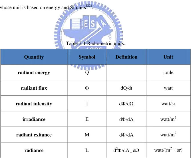
Radiometric quantities include radiant energy, radiant flux, radiant intensity, irradiance, radiant exitance, and radiance. Table 2-1 shows these fundamental radiometric quantities whose unit is based on energy and SI units[22].

Table 2-1 Radiometric units.

Quantity Symbol Definition Unit

radiant energy Q joule

radiant flux  dQ/dt watt

radiant intensity I d/d watt/sr

irradiance E d/dA watt/m2

radiant exitance M d/dA watt/m2

radiance L d2/dA d watt/(m2 sr) ( t: time, : solid angle, A: area )

13

Radiant energy Q defines the energy of a collection of photons (as in a laser plus). Radiant flux  is the measure of total power of radiation. The power may be the total emitted from a source or the total landing on a particular surface. Basing on radiant energy Q and radiant flux , the other quantities are derived by various geometric normalizations.

Radiant intensity I is generally used to describe the characteristics of sources whose size is infinitesimal, such as a point source. The definition of I is the radiant flux per unit solid angle of a specified surface which the radiation is incident upon or passing though, as shown in Fig.2-1(a).

Irradiance E describes radiation distribution on a received plane. The definition is the radiant flux per unit area of a specified surface which the propagating radiation is incident on or passing though, as shown in Fig. 2-1(b).

If the radiant flux leaving the plane per unit area is considered, the term radiant exitance

M is used instead of irradiance E but is expressed by the same equation. Radiant exitance M

describes radiation distribution on the plane which emits the radiation, as shown in Fig. 2-1(c).

When an extended source, such as a planar source, is considered, radiance L is used to describe its characteristic. The definition is the radiant flux per unit project area and per unit solid angle of a specified surface which the propagating radiation is incident on or passing through, as shown in Fig. 2-1(d). The projected area of the plane element equals to dAcos, where  is the angle between the normal of the plane element and the direction of observation.

14

Photometric quantities

For human visual system, the responses to the optical radiation with different wavelengths are dissimilar. Photometric quantity is an operationally defined quantity designed to represent the way in which the human visual system evaluates the corresponding radiometric quantity. Accordingly, it is also called a psychophysical quantity. In particular, the optical radiation within the wavelengths range between 380 nm and 780 nm, so-called visible light, are discussed by photometry.

Photometric quantities include luminous energy, luminous flux, luminous intensity, illuminance, luminous exitance, and luminance. In geometric terms, the definitions of these photometric quantities are the same as for the corresponding radiometric quantities. Table.2-2

Solid angle element d Radiant flux d

(a) Radiant intensity

Radiant flux d Plane element dA (b) Irradiance Radiant flux d Plane element dA (c) Radiant exitance Radiant flux d Plane element dA (d) Radiance 

15

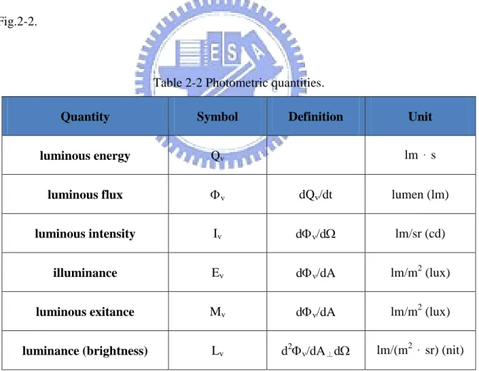
shows the photometric quantities whose unit is based on lumen (lm)[22]. Lumen is defined as „luminous flux emitted into a solid angle of one steradian by a point source whose intensity is 1/60 of the intensity of 1 cm2 of a blackbody at the temperature of platinum (2042K) under a pressure of one atmosphere.‟

From the definition of lumen, the maximum value of spectral luminous efficiency could be determined. At the wavelength 555 nm, which corresponds to the maximum spectral efficiency of human eyes, 1 watt is equal to 680 lumens. Therefore, the luminous flux v

emitted by a source with a radiant flux  is given by:

680 ( ) ( )

v V   d

 



 , (2-13)

where  is the wavelength and V() is the spectral luminous efficiency function as shown in

Fig.2-2.

Table 2-2 Photometric quantities.

Quantity Symbol Definition Unit

luminous energy Qv lm s

luminous flux v dQv/dt lumen (lm)

luminous intensity Iv dv/d lm/sr (cd)

illuminance Ev dv/dA lm/m2 (lux)

luminous exitance Mv dv/dA lm/m2 (lux)

luminance (brightness) Lv d2v/dA d lm/(m 2

sr) (nit) (t: time, : solid angle, A: area)

16

Fig. 2-2 Human visual response function.

2.3 Bidirectional transmission and reflection distribution function

Basing on radiometry and photometry, the bidirectional transmittance and reflectance distribution functions (BTDF and BRDF) are developed to describe scattered light distributions[23]. The BTDF describes the transmissive characteristic of a sample, while the BRDF indicate the reflective characteristic of a sample. In this thesis, the wavelength corresponded BTDF and BRDF were adopted to describe the phosphor film‟s light-scattering characteristics which combine diffusing process with wavelength-converting mechanism.

The defining geometry of BTDF and BRDF is shown in Fig. 2-3, where the subscripts i,

t, and r are denoted for incident, reflected and transmitted quantities, respectively. The

notation



is the azimuthal angle between light direction and the normal direction of sample surface, and  is the polar angle on the sample surface. If a incident light with luminous flux

v,i and wavelength i illuminating on the sample with area A is considered, the transmitted

and reflected light scattered from the sample could be described by BTDF and BRDF which are defined as follows:

17 , , , , ( , , ) ( ) / ( , , , , , ) ( , , ) ( ) cos v t t t t v t t t i i t t i t v i i i i v i i t L d d BTDF E

  



     

  





      (2-14) , , , , ( , , ) ( ) / ( , , , , , ) ( , , ) ( ) cos v r r r r v r r r i i r r i r v i i i i v i i r L d d BRDF E

  



     

  





      (2-15)

where t and r are the wavelengths of transmitted and reflected light, Ev,i is the illuminance

on the sample plane due to incident light, and Lv,t and Lv,r are the luminance of transmitted and

reflected light at the particular received angles, respectively.

incident light



v,i



i

reflected light



v,r



r

transmitted light



v,t



t

A

d



t

d



r



i



i



r



t



t

Normal

direction



r

sample

Fig. 2-3 Schematic diagram of BTDF and BRDF.

BTDF and BRDF describe the luminance distributions of transmitted and reflected light scattered from a sample. Besides, the terms d_{v t,}(_t) /_{v i,}(_i)and d_{v r,} (_r) /_{v i,}(_i) in BTDF and BRDF mean the transmittance and reflectance of the transmitted and reflected light in (t , t) and (r , r) direction, which could be obtained by measuring illuminance of

18

r indicate the wavelengths corresponded relation of incident light and the scattered light.

Therefore, the BTDF and BRDF provide a convenient solution to describe the way in which the light is reflected and refracted by a sample even propagating in different wavelengths with the incident light. Accordingly, the scattering specification of conventional diffuser films and phosphor films could be generated, and then be utilized by optical designers, manufacturers, and users to communicate and check requirements.

In this thesis, the BTDF and BRDF of phosphor films are measured by our designed BTDF measurement systems and a conoscopic system operating under trasnmissive and reflective mode. The measured BTDF and BRDF data were then imported to out optical design software, LightToolsTM, to develop the simulation models that could describe the light-scattering characteristics of phosphor films. Thus, we could start our design and optimization of UFL and BFL backlight systems.

2.4 Colorimetry

Colorimetry is the science relating color comparison and matching. As mentioned earlier, for visible light, the optical radiations within wavelengths ranging from 380 nm to 780 nm, the photometric quantities have provided measures to describe the amount of energy. However, in human visual system, the optical radiations arouse not only intensity response (brightness) but also chromatic response (chromaticity). Therefore, in this thesis, colorimetry is imported to specify the chromatic performance of backlight units. The CIEXYZ and CIELUV color spaces, which have been developed for denoting colors numerically, are described in the following paragraphs.

CIEXYZ color space

The CIE XYZ system, created by the International Commission on Illuminance (CIE) in 1931, is one of the first mathematically defined color systems that specify colors

19

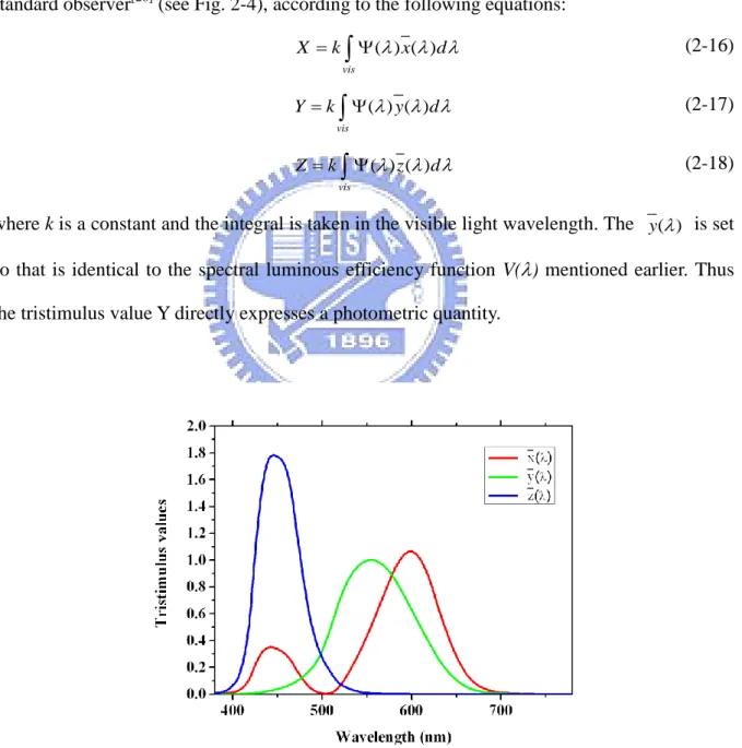
numerically[ 24]. The human eye has receptors for short (S), middle (M), and long (L) wavelengths. Thus in principle, three parameters describe a color sensation. The tristimulus values of a color are the amounts of three primary colors in a three-component additive color model needed to match that test color[25]. In the CIE XYZ system, the tristimulus values are called X, Y, and Z. The tristimulus values for a color with a stimulus ( ) can be derived from the color matching functions, the numerical description of the chromatic response of standard observer[26] (see Fig. 2-4), according to the following equations:

( ) ( ) vis X k



  x  d (2-16) ( ) ( ) vis Yk



  y  d (2-17) ( ) ( ) vis Z k



  z  d (2-18)

where k is a constant and the integral is taken in the visible light wavelength. The y( ) is set so that is identical to the spectral luminous efficiency function V() mentioned earlier. Thus

the tristimulus value Y directly expresses a photometric quantity.

20

Basing on CIE XYZ system, a color could be specified by utilizing the tristimulus values

X, Y, and Z in a three-dimensional color space, called CIEXYZ color space. Besides, for

convenient descriptions of colors, a color space specified by x, y, and Y, known as CIExyY color space, was derived[27]. The x and y are defined as following equations:

X x X Y Z    (2-19) Y y X Y Z    (2-20) 1 Z z x y X Y Z       (2-21)

The z coordinate could be omitted by providing Y parameters which is a measure of the luminance of a color. Accordingly, the chromaticity description of a color could be expressed more conveniently in a two-dimensional plane, which is called CIE xy chromaticity diagram and be widely used in practice (see Fig.2-5).

Fig. 2-5 xy chromaticity diagram of CIE XYZ color system.

However, the xy chromaticity diagram is highly non-uniform and has been found to be a serious problem in practice[ 28 ]. The color difference between two colors could not be calculated by using CIEXYZ color space or xy chromaticity diagram. Therefore, a uniform

21

color space, the CIELUV color space, is proposed to replace the non-uniform CIEXYZ color space.

CIELUV color space

The CIELUV color space adopted by CIE in 1976 is an attempt to define an encoding with uniformity in the perceptibility of color difference[29]. Such a uniform color space is based on a simple-to-compute transformation of the 1931 CIEXYZ color space[30,31]. For the non-linear relations from CIEXYZ color space to CIELUV color space, the three-dimensinal orthogonal coordinates adopted in CIELUV color space are defined as follows[32]:

1/3 * 116( / n) 16 L  Y Y  (2-22) * 13 *( ' n') u  L u u (2-23) * 13 *( ' n') v  L v v (2-24)

where u’ and v’ is the coordinates of two-dimensional u’v’ chromaticity diagram (Fig.2-6) defined as Equation 2-25 and 2-26, Yn, un’, and vn’ are the tristimulus value and the

chromaticity coordinates u’ and v’ of reference white, respectively.

4 ' 4 15 3 X u X Y Z    (2-25) 9 ' 15 3 Y v X Y Z    (2-26)

Basing on the uniform CIELUV color space, the color difference of two colors could be calculated. The color difference u’v’ between two colors (u1’,v1’) and (u2’,v2’) at the u’v’

chromaticity diagram is defined as[33]:

2 2 2 2

1 2 1 2

' ' ( ') ( ') ( ' ') ( ' ')

u v u v u u v v

         (2-26)

In this thesis, Equation 2-26 is imported to judge the chromatic performance of the backlight units.

22

Fig. 2-6 u’v’ chromaticity diagram of the CIELUV color system.

2.5 Summary

Table.2-3 summarizes the principles mentioned earlier in this chapter. In this thesis, ray-tracing method was used to design backlight system in this thesis. By Snell‟s law, law of reflection, and Fresnel‟ equations, the propagation trajectory and the carried energy of light

could be calculated. Besides, basing on radiometry and photometry, the

wavelength-corresponded BTDF and BRDF provided a convenient solution to describe the scattering characteristics of phosphor films. Therefore, the ray-tracing based optical design software, LightTools, was utilized to simulate a backlight system. And then the measured BTDF and BRDF data were imported to LightTools for development of simulation model for design and optimization of the UFL system and the BFL system. Accordingly, the CIELUV color space and the color difference u’v’ were utilized to judge the optical performances of the backlight units. The wavelength corresponded BTDF and BRDF of phosphor films are the most important part for developing simulation models of UFL system and BFL system. Therefore, the measurement instruments will be discussed in the following chapter.

23

Table 2-3 Function of applied principles.

Method Principle Function

Ray tracing

Snell‟ law

Calculating propagation trajectory and carried energy of light. Law of reflection

Fresnel‟s equations

Radiometry & Photometry

BTDF _{Characterizing light scattering}

properties of phosphor films. BRDF

Colorimetry

CIELUV color space _{Specifying chromaticity performance}

of backlight output distribution. Color difference (u’v’)

24

Chapter 3

BTDF and BRDF Measurement Instruments

A phosphor film simulation model was essential for designing and optimizing the UFL and BFL systems. In order to specify the light scattering characteristics of phosphor films and develop phosphor film models, BTDFs and BRDFs were first measured. The BTDFs and BRDFs were measured using a conoscopic system and a customized BTDF measurement system. Then, the measured BTDF and BRDF data were imported into the optical design software, LightTools, to start modeling. The principle of conoscopic system and the specially designed BTDF measurement system will be presented in this chapter.

3.1 Conoscopic system

Transmissive mode

A conoscopic system was utilized to measure the angular light distributions of samples. The optical radiations within wavelength ranges between 380 nm to 780 nm, known as visible light, were measured by this system. The measuring mode of this system could be classified into transmissive and reflective modes. In transmissive mode (as shown in Fig. 3-1), a Fourier transform lens was adopted to transform the received light into a two-dimensional pattern. Each light beam emitted from the test area at incident angle, θ, could be focused on the focal plane at the same azimuth and at a position x=F(θ). Then, a relay system was utilized to project this transform pattern onto a CCD-array detector. In this transform pattern, each area corresponded to one specific light propagation direction. Thus, when this pattern was projected on the CCD-array detector, the light intensity and chromaticity versus dissimilar viewing directions were obtained

25

measurement system which will be described later in this chapter, the BTDFs of phosphor films and the optical performance of backlight systems were measured using the conoscopic system in the transmissive mode directly.

Fig. 3-1 Schematic of the conoscopic system in transmissive mode.

Reflective mode

Besides the transmissive mode, a reflective mode in the conoscopic system is available to measure the angular distributions of light reflected from samples. In the reflective mode (as shown in Fig. 3-2), a light source is implemented at the Fourier transform plane to illuminate samples from inside the conoscopic system. A collimated light struck the sample surface with a tiny illuminated area was reflected back into the conoscopic system. Therefore, the angular distribution of these reflected lights were obtained with the CCD-array detector. The illuminating angle, θ, of the built-in source was easily varied by controlling the position of the light source on Fourier transform plane. Therefore, the BRDFs of a sample were measured. In this experiment, the BRDFs of phosphor films and reflectors were obtained by measuring the angular distributions of reflected light under the reflective mode of conoscopic system.

26

Fig. 3-2 Schematic of the conoscopic system in reflective mode.

3.2 BTDF measurement system

To measure the BTDFs of phosphor films, a device which could provide a collimated light in different illuminating angles was required. The BTDF measurement system was designed and fabricated for this purposes, as shown in Fig. 3-3.

In the BTDF measurement system, an LED stage was connected to a slippery track located on the side plane of the system. The rail of the slippery track was an arc and the LED stage slid along this rail. Besides, an aperture with small diameter is placed on the exit plane of the LED and a circular hole with a tiny surface area was bored on the top plate of system. In this structure, the sample placed on the top plate of this measurement system was illuminated using a collimated light whose illuminating angle could be varied from 0 to 70 degrees.

When measuring BTDFs of phosphor films, the BTDF measurement device was placed under the conoscopic system to serve as a light source. The optical properties in each viewing direction were measured using the conoscopic system in transmissive mode. A photograph of the experimental setting is shown in Fig. 3-4.

27

Slippery track

(a) Front view (b) Side view

Fig. 3-4 Diagram of BTDF measurement.

Conoscopic system Measured sample (e.g. phosphor film) Our designed light

source device

LED stage Aperture

28

3.3 Summary

To develop a phosphor film simulation model and design the UFL and BFL systems, the scattering characteristics of phosphor films were first specified. A BTDF measurement system was utilized to measure the BTDF value of phosphor films to import into LightTools to build corresponding model. In addition, the conoscopic system was also used to measure the BRDF of phosphor film, BRDF of the reflector, and other backlight system optical properties, such as angular luminance distribution, color information. Accordingly, optical properties of the UFL system and the BFL system were simulated and analyzed.

29

Chapter 4

UV Excited Flat Lighting (UFL) System

Basing on research of external photo-fluorescent technology, the UV Excited Flat Light (UFL) system was proposed. By the large-sized remote phosphor layer which simultaneously converted UV light into visible light and diffused the excited visible light, the UFL system emitted light as a planar light source directly. However, the specific optical properties in UFL system were difficult to be simulated in traditional simulation method. Thus, a simulation model was developed to describe the light-scattering characteristic of phosphor films in the UFL system and further optimize such backlight system.

4.1 Light-emitting mechanism of UFL system

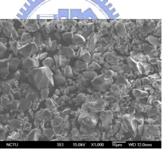
The UFL system was similar to the traditional CCFL backlight but differed in the light source. Instead of using the conventional CCFL, the UFL system consisted of UV lamps and phosphor layer coated outside the lamps. Fig. 4-1 shows the configuration of the UFL system where the UV lamps are placed inside the backlight cavity, and two phosphor layers are coated on the bottom reflector and under the top PET plate, respectively. Fig.4-2 shows the top view of the phosphor layer captured by a Scanning Electron Microscope (SEM). The main differences from a CCFL backlight were that the phenomena of the UV light in free space

were different from the visible light, and the light propagation included

wavelength-converting process on phosphor layers. In the UFL system, the phosphor layers played the roles as the wavelength converters (for UV light) and the diffusers (for visible light), simultaneously. When the UV light radiated from UV lamps irradiated the phosphor layers around the cavity, the Lambertian visible light was excited from the phosphor layers.

30

When the visible light irradiated the phosphor layers, the visible light was diffused by the phosphor layers again. Since the visible light was redistributed on the flat phosphor layers, the UFL system yielded higher uniformity than the conventional CCFL backlight.

Fig. 4-1 (a) Scheme of UFL system; (b) Cross-structure of UFL with relative modeling steps.

Fig. 4-2 Top view of the phosphor layer captured by a scanning electron microscope (SEM).

4.2 Simulation model of UFL system

To design the geometrical structures and optimize the optical performances of the UFL system, a simulation model which could describe the light-scattering properties of phosphor film was developed. The simulation software, LightTools, was adopted to develop this simulation model. LightTools can model real objects and follows the ray-tracing method in

Reflector Bottom Phosphor UV Lamps PET Plate Top Phosphor x y C D E A B

x

(a) _(b)

31

simulation. Fig. 4-2 shows the scheme of the modeling process, where symbols A-E indicate the internal processes relative to the A-E in Fig. 4-1(b). First of all, the mechanism of a unit-lamp module was created in the software. The BSDFs (which include BTDF and BRDF) of phosphor layers for visible-to-visible light and UV-to-visible light were respectively applied to the simulation model. We assumed the two phosphor layers were two emitters (A and B) to simply wavelength-converting mechanism, and the visible light was radiated to the three surfaces (C-E). The ray-tracing was performed in three parts relative to the three emitting modes, and the three results of the unit-lamp model were combined into one output. Finally, the total output of a multi-lamps module was calculated from the convolution between the unit-lamp normal luminance distribution and a one-dimensional comb function:

( , ) ( , ) ( , ) ( , )

total u u

m m

I x y I x y 



 xmd y 



I xmd y (4-1)

where m and d indicated the m-th lamp and the lamp period of the multi-lamp module, and

Itotal and Iu were the total light distribution and the unit-lamp light distribution. Accordingly,

this method provided a flexible way to simulate in the system with variant lamp numbers.

Fig. 4-3 Flowchart of modeling process of UFL system

Unit-Lamp Module

A. Top Emitter

B. Bottom Emitter

BSDF

(UV light  Visible light)

C. Up Propagation

D. Down Propagation

E. Up Propagation

BSDF

(Visible light  Visible light)

Convolution I Comb Correlation Coefficient Output > 95% < 95% Module Multi-Lamp Module

32

4.3 BTDF and BRDF measurement results

The phosphor layers were characterized by the measured BSDFs. The BSDFs (which include BTDF and BRDF) of phosphor layers for UV-to-visible light and visible-to-visible light were respectively measured and then be applied to the phosphor simulation model of the UFL system.

BTDF/BRDF of phosphor film for UV-to-visible light

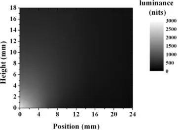
The BTDF/BRDF of phosphor films were classified into two parts: the BTDF/BRDF for 1) visible-to-visible light and 2) UV-to-visible light. The BTDF for UV-to-visible light was measured as the database from a unit-lamp UFL module as shown in Fig. 4-3. The height and position were varied from 0 to 18 mm and 0 to 24 mm respectively. The conoscopic system was utilized to measure the angular distribution of output light (visible light) at each measuring point. The measured BTDF data are shown in Fig. 4-4 and 4-5. Normal direction luminances of each measured point decreased with the increased heights and positions. Besides, by wavelength-converting mechanism, the angular distributions of each measured point were close to the Lambertian distribution. The UV-excited visible light emitted in all directions on both side of phosphor film because of the wavelength-converting mechanism. Therefore, in our experiment, the BRDF of phosphor film for UV-to-visible light was assumed to be equal to the measured BTDF data of phosphor film for UV-to-visible light.

Fig. 4-4 Schematic BTDF measuring process in a unit-lamp UFL module. Height

Position Conoscopic system

UV Lamp

33

Fig. 4-5 Measured BTDFs (luminance in normal direction) of phosphor film for UV-to-visible light.

Fig. 4-6 Measured BTDFs (normalized angular distribution) of phosphor film for UV-to-visible light at 0-mm and 12-mm position with 10-mm height.

BTDF/BRDF of phosphor film for visible-to-visible light

In UFL system, the phosphor films not only converted UV light into visible light but also scattered the visible light simultaneously. Besides, the reflector at bottom would reflect the visible light also. Therefore, the BTDF/BRDF of phosphor films and the BRDF of reflector for visible-to-visible light were measured using the conoscopic system and then be imported into phosphor simulation model individually.

34

0

10

0

10

By Mie theory[34], the phosphor particle (particle size = 10um) would diffuse the incident visible light. The measured BTDF and BRDFs of the phosphor film and the reflector for visible-to-visible light are shown in Fig. 4-6. By light-scattering mechanism, the BTDF of the phosphor film differed from that of the same phosphor film under wavelength-converting mechanism. The BTDF for visible-to-visible light exhibited directional distribution and had transmission light peaks at incident angles 0° to 40°, while the BTDF for UV-to-visible light exhibited the Lambertian distribution at each incident angle. The phosphor film had reflectance light peaks at incident angles 0° to 10°. Besides, because the reflector had white particles on its surfaces, the specular reflections and the diffusions were occurred simultaneously.

(a)

(b) (c)

Fig. 4-7 Measured BTDF of (a) phosphor film and BRDFs of (b) phosphor film and (c) reflector, for visible-to-visible light.

35

4.4 Simulation and experimental results

By importing the measured BTDF and BRDF data of the phosphor film, the UFL system simulation model was established. Accordingly, the geometrical structure of the UFL system was designed and optimized by this simulation model.

4.4.1 Simulation and optimization results

To simplify the optimizing process, a UFL system with 4 pieces of UV lamps was designed and optimized in the simulation environment. Therefore, the simulation results could be scaled up and applied into a 32-inch UFL system.

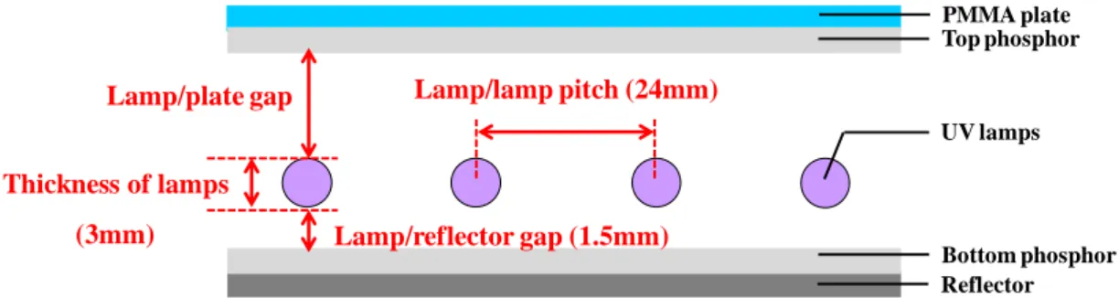
The simulation setups of the 4-lamps UFL system are shown in Fig.4-7 and Table 4-1, respectively. As current designs of the conventional 32-inch direct-emitting type backlight system with 16 pieces of CCFL lamps, the lamp pitches of the UV lamps in the UFL system were fixed at 24mm. Besides, the lamp/reflector gap was also fixed at 1.5mm as the design of the conventional backlight system. Then, in the optimizing process, the lamp/plate gap was altered and the on-axis luminance distribution was measured for discussing optical performances of the UFL system. In addition, the 80%-uniformity was the critical condition for human eye in perceiving a uniform/non-uniform luminance distribution. Therefore, the uniformity was also calculated for examining the UFL system.

Fig. 4-8 The configuration of the 4-lamps UFL system in simulated environment. Lamp/lamp pitch (24mm) Lamp/plate gap Lamp/reflector gap (1.5mm) Thickness of lamps (3mm) Reflector Bottom phosphor Top phosphor PMMA plate UV lamps

36

Table 4-1 Specification of the 4-lamps UFL system in simulated environment.

Parameter Value (mm)

Thickness of lamp 3

Lamp/lamp pitch 24

Lamp/reflector gap 1.5

Lamp/plate gap 2.8/ 5.8/ 8.8/ 11.8/ 14.8

The simulated on-axis luminance and the calculated lamp-mura uniformity of the 4-lamps UFL system are shown in Fig.4-8 and Fig.4-9, respectively. The lamp-mura uniformity was defined as the following equation and calculated between two lamps at the central position:

min

max between two lamps

L Uniformity L  , (4-2)

where the Lmin and Lmax indicated the minimum and maximum luminance between 3x3 LED chips, respectively. The simulation results indicated that a larger lamp/plate gap of the UFL system induced a more uniform output distribution. By simulation results, the UFL system exhibited 89% lamp-mura uniformity with 5.8mm lamp/plate gap. Besides, the lamp-mura uniformity of the UFL system was higher and lower than 80% when the lamp/plate gap was larger and smaller than 5.8mm. Accordingly, the 5.8-mm lamp/plate gap was chosen as the appropriate value for the UFL system in developing a slim-format backlight system

37

Fig. 4-9 The normalized on-axis luminance of the simulated 4-lamps UFL system (with different lamp/plate gap values).

Fig. 4-10 The uniformity of the simulated 4-lamps UFL system (with different lamp/plate gap values).

38

4.4.2 Simulation model verification

A 4-lamps UFL system was fabricated in order to further verify the accuracy of the developed UFL system simulation model. As shown in Fig.4-10, the simulation result was compared with the experimental result at 5.8-mm lamp/plate gap of the 4-lamps UFL system. To determine the similarity between the simulation model pattern and the experimental measurement, the correlation coefficient was applied:

2 2 ( , ) ( , ) , ( , ) ( , ) s m s m x y s m s m x y I x y I I x y I Correlation Coefficient I x y I I x y I                     





(4-3)

where x and y indicated the x-th and y-th pixel on the output mesh, Is and Im were the light

distribution of the simulation and measurement results, and I (s I ) was the mean value of m s

I (I_m), respectively. The calculated correlation coefficient between the simulated and experimental results was 95.48%. And the measured uniformity was 90% between the two lamps at the central position.

The other simulated results with different lamp/plate gap values were also verified by calculating the correlation coefficient (as show in Table 4-2). All of these simulation results were correspond to the experimental results and had correlation coefficients higher than 95%. Therefore, the UFL simulation model was available for designing and optimizing purpose of the UFL system. Moreover, the 5.8mm lamp/plate gap was verified that it was appropriate for designing the slim format UFL system.

39

Fig. 4-11 Simulated and experimental on-axis luminance results of the 4-lamps UFL system. (with lamp/plate gap=5.8mm and lamp/lamp pitch=24mm)

Table 4-2 Correlation coefficients between simulation and experimental results.

Lamp/plate gap (mm) 5.8 8.8 11.8 14.8

Lamp/lamp pitch (mm) 24 24 24 24

Correlation coefficient (%) 95.48 96.66 96.00 97.24

4.4.3 Experimental results of optimized UFL module

According to the optimized results, a 32-inch UFL system with 5.8-mm lamp/plate gap was demonstrated. Moreover, a conventional CCFL backlight system (with diffuser plate) was arranged with same geometrical structure parameters for comparison. Since the visible light was redistributed on the flat phosphor layers, the UFL system emitted light as a planar source directly (as shown in Fig.4-11). Thus, the UFL system yielded higher uniformity than the conventional CCFL backlight system did. Fig.4-12 shows the measured luminance results of the slim-format UFL and CCFL systems. At the optimized lamp/plate gap (5.8mm), the