應用多方向量分析分析污染檢測數據

(1)

國立交通大學

環境工程研究所

碩士論文

應用多方向量分析分析污染檢測數據

The Analyses of Sampling Data Using

Polytopic Vector Analysis

研究生：莊敏筠

指導教授：葉弘德教授

(2)

應用多方向量分析分析污染檢測數據

The Analyses of Sampling Data Using

Polytopic Vector Analysis

研究生：莊敏筠

Student：Min-Yun Chuang

指導教授：葉弘德

Advisor：Hund-Der Yeh

國立交通大學

環境工程研究所

碩士論文

A Thesis

Submitted to Institute of Environmental Engineering

College of Engineering

National Chiao Tung University

in Partial Fulfillment of the Requirements

for the Degree of

Master of Science

in

Environmental Engineering

August, 2007

Hsinchu, Taiwan

中華民國九十六年八月

(3)

應用多方向量分析分析污染檢測數據

研究生：莊敏筠指導教授：葉弘德

國立交通大學環境工程研究所

摘要

鑒定化學污染源與瞭解污染團在時空上的分佈，在環境污染領域

是重要且新受矚目的問題。在多重污染源地區，環境工程師面臨著如

何鑒定複雜地形的污染源型態。如果污染源具有獨特的化學指紋，即

可藉由多變數統計分析方法來進一步解決環境指紋問題。

多方向量分析(Polytopic Vector Analysis)是一種鑑定污染源化學

指紋的多變量分析統計方法。假定某一混合系統，多方向量分析可用

來計算三個重要參量：(1)來源(後端成分)個數、(2)各後端成分的化學

指紋組成、以及(3)不同樣本中來自各來源的濃度相關比例。

本研究應用多方向量分析，分別針對兩個研究案例做分析(I)客雅

溪流域重金屬檢測數據，以及(II)新竹科學園區地下水有機污染檢測

資料。

近年來，在新竹香山海域養殖的牡蠣及沈積物的銅含量皆出現顯

著增高的趨勢。綠牡蠣體內伴隨著高濃度的銅含量，不但威脅消費者

健康且影響漁民每年三百多萬美金產值。香山牡蠣銅污染的來源是長

久被關切且極需解決的問題。雖然在過去的研究曾指出香山海域銅污

染可能源自於新竹科學園區或香山工業區，然而卻缺少強而有力的證

據指出確切的污染者。於 2006 年檢測客雅溪及其支流的十二組數

(4)

據，這十二組數據分別來自於不同兩組研究團隊的檢測成果。本研究

目的在於利用統計方法-多方向量分析，鑑定綠牡蠣組織內的重金屬

銅之來源。第一組及第二組數據，分別在客雅溪沿岸檢測共 6 個水樣

及 7 個懸浮固體樣本，採樣時間為 2006 年四月，每個取樣分析 18 種

重金屬項目(鋅、銅、鉛、鐵、鋁、錳、鎘、鍶、鉻、鋇、鎳、銀、

錫、砷、釩、鎢、鎵及鉬)。第三組到第八組數據，沿客雅溪流域 7

個取樣點，採樣時間為 2006 年二月至七月；第九組到第十二組數據，

沿客雅溪流域 8 個取樣點，採樣時間於 2006 年八月至十一月，每個

水樣分析六個項目(懸浮固體、溶氧、生化需氧量、氨氮、銅及砷)。

由多方向量分析結果顯示，新竹科學園區為綠牡蠣中銅的主要來源。

在第二個研究案例，係應用多方向量分析針對新竹科學園區地下

水污染檢測資料作分析，利用計算係數以及因子負荷係數判定該工業

區地下水有機污染物資料，鑒定出有六個有機污染物指紋，進而計算

出各後端成分在地理上的分佈。因此，利用多方向量分析可決定後端

成分的個數，並且發展出一個地下水污染物的混合模式，以模擬地下

水污染源化學指紋與污染團在空間上的分佈。

(5)

The analyses of sampling data using

Polytopic vector analysis

Student: Min-Yun Chuang Advisor: Hund-Der Yeh

Institute of Environmental Engineering

National Chiao Tung University

ABSTRACT

Identification of chemical contaminant sources is an important environmental

problem. Given multiple sources in a field area, the environmental engineer is faced

with the challenge of identification and mapping multiple plumes with overlapping

geographic distribution. If a contaminant source is characterized by a distinctive

spectrum of chemicals, then the environmental chemical fingerprinting problem may

be addressed through a multivariate statistical approach.

Polytopic vector analysis (PVA) is a statistical pattern recognition technique for

multivariate data used to identify fingerprints of contaminant sources. Given a

mixed system, PVA is used to determine three parameters of interest in a mixed

system: (1) the number of sources (end-members), (2) the composition of each source,

(6)

In this study, polytopic vector analysis is applied to analyze two problems. In the

first problem, the copper source of green oyster in Hsianshan wetland is identified

while in the second problem the groundwater contamination by organic chemicals in

Hsinchu science park is analyzed.

In recent two decades, the copper concentrations in both the oyster organs and

sediment were very high in the Hsianshan coastal area, Taiwan. The oyster with

high concentration of copper poses not only a threat to human health but also results

in an annual loss of about 3.1 million US dollars. What is the source of copper in the

Hsianshan oyster is a question of long standing and tough problem to be solved.

Previous studies indicated that the copper source originated from either the Hsianshan

industrial park (HIP) or the Hsinchu Science Park (HSP) is responsible for the

contamination in Hsianshan coastal area. Although several investigations had been

conducted for identifying the copper source of green oyster; however, there was no

clear evident or result to show who is responsible for the copper pollution. In order

to search for the source of copper, the water and suspended solid samples were

collected and analyzed. Water samples mainly collected from the Keya stream and

(7)

collected from the Keya stream and coastal area of Hsianshan. Totally 12 sets of

water and suspended solid sample data were available. The Data Set 1 contains

water samples taken from 6 different sites along the Keya stream, Hsinchu while the

Data Set 2 has suspended solid samples taken from the same stream at 7 different sites.

Both two data sets are analyzed for eighteen heavy metals including Zn, Cu, Pb, Fe,

Al, Mn, Cd, Sr, Cr, Ba, Ni, Ag, Sn, As, V, W, Ga, and Mo. The Data Sets 3 to 8 were

sampled at 7 locations along the Keya stream during February to July, 2006. The

Data Sets 9 to 12 were collected at 8 locations, where 7 locations were the same as

those taken above and one extra location was at Yuchegou creek, during August to

November, 2006. Those ten data sets, Data Sets 3 to 12, were taken and analyzed for

six items (SS, DO, BOD, NH3-N, Cu, As). The purpose of this study is to identify

the copper source based on those sample data using a multivariable statistical analysis

called polytopic vector analysis (PVA). The results of PVA indicate that a significant

part of copper comes from HSP and a minor part of copper is from Yuchegou creek.

In the second problem, the study applies PVA to analyze the concentration data

taken from HSP, Taiwan. Based on inspecting the coefficient of determine (CD

(8)

identified. Moreover, the geographic distribution of each end-member can be

presented. Thus, this method (PVA) can develop a groundwater mixing model by

searching for end-members. In addition, this mixing model can identify chemical

contaminant sources and map multiple plumes with overlapping geographic

(9)

致謝

這本碩士論文，我要獻給我最愛的父母親。感謝您們不辭辛勞的工作，就為了給我們最好的教育環境。也因為您們的教誨，讓我有向上的動力。能夠完成這本論文，首先要感謝我的指導教授葉弘德老師，老師總能在適時提供我論文的方向，並細心的指正論文的每個細節，才能讓論文有今天這麼完整的面貌。在老師那邊也學習到很多做研究的謹慎的態度，更獲得許多寶貴的經驗。另外，也要感謝海洋大學的陳明德教授，教導統計觀念及提供軟體讓我能突破研究最開始的瓶頸。再來要非常感謝我的可愛的 GW Group-智澤學長、彥禎學長、雅琪學姊、彥如學姊、士賓、博傑、其珊、仲豪、珖儀及跟我一起打拼兩年的隊長毓婷！謝謝你們平時的鼓勵及照顧，我們一起登玉山、遊司馬庫斯的美好經驗，相信永遠都會存在我們的心中！再來我要特別感謝，這六年來一路陪伴我的瑞元，在最重要的時刻你總是給我最棒的精神鼓勵及支持，讓我有勇氣突破！希望我的致謝能夠真實的傳達我最真摯的感謝。在交大的六年，如今要畫下一個句點。但，這個句點代表著下個人生階段的起點敏筠謹致於交通大學環境工程研究所 2007年8月

(10)

摘要 ... I

ABSTRACT... III

致謝...VII

TABLE OF CONTENTS... VIII

LIST OF TABLES...X

LIST OF FIGURES ... XIII

PREFACE ...1

PROBLEM I...2

CHAPTER 1 INTRODUCTION...3

1.1 Hsinchu city ...3

1.2 Hsinchu science park and Hsianshan industry park ...4

1.3 Hsianshan wetland and green oysters ...6

1.4 Oysters character ...8

1.5 Two green oyster investigation projects ...10

1.6 Polytopic vector analysis ...14

1.7 Objectives...16

CHAPTER 2 MATERIAL AND METHOD...17

2.1 PVA Formalism ...17

2.2 Matrix adjustments...17

2.3 Polytopic Vector Analysis ...18

2.4 Determining the number of end-members...19

CHAPTER 3 RESULTS AND DISCUSSION ...23

3.1 PVA results based on Huang et al.’s data...23

3.1.1 The chemical pattern of Data Set 1 ...23

(11)

CHAPTER 4 CONCLUSIONS ...40

PROBLEM II ...41

Groundwater Contamination by Organic Chemicals in Hsinchu

Science Park ...41

CHAPTER 1 INTRODUCTION...42

1.1 Hsinchu Science Park ...42

1.2 Polytopic vector analysis ...43

1.3 Objective ...45

CHAPTER 2 MATERIAL AND METHOD...46

2.1 Matrix adjustment ...46

2.3 Determining the number of end-members...48

CHAPTER 3 RESULTS AND DISCUSSION ...51

3.1 Determination of number of chemical fingerprints ...51

3.2 End-member fingerprint composition and geographic distribution 52 CHAPTER 4 CONCLUSION...55

REFERENCES...56

(12)

LIST OF TABLES

TABLE 1. The copper concentrations of oyster and sediment in Hsianshan area form 1987 to 2006...60

TABLE 2. The location of sampling points a. ...61 Note: The distance is measured from the confluence of Nanman creek and Keya stream. The minus symbol represents the upstream direction. ...61

TABLE 3. The copper concentrations from February to December, 2006 collected from 7 sampling points along Keya stream (BEPH, 2006)...62

TABLE 4 The concentration data of 6 chemical items of Data Set 3 to Data Set 12 (BEPH, 2006) ...63

TABLE 5. End-member fingerprint compositions (in percent) analyzed through PVA of Data Set 1, 6×18 data matrix, 6 end-member model. Each column sums to 100%. ...66

TABLE 6. End-member fingerprint compositions (in decimal percentages)

analyzed through PVA of Data Set 1, 6×18 data matrix, 6 end-member model. ..67

TABLE 8. End-member fingerprint compositions (in decimal percentages)

analyzed through PVA of Data Set 2, 7×18 data matrix, 7 end-member model. ..69

TABLE 10. End-member fingerprint compositions (in decimal percentages) analyzed through PVA of Data Set 3, 7×6 data matrix, 6 end-member model. ....70

(13)

TABLE 23. End-member fingerprint compositions (in percent) analyzed through PVA of Data Set 10, 8×6 data matrix, 6 end-member model. Each column sums

(14)

to 100%. ...77

TABLE 24. End-member fingerprint compositions (in decimal percentages) analyzed through PVA of Data Set 10, 8×6 data matrix, 6 end-member model. ..77

TABLE 29. The 13 eigenvalues, the cumulative percent variance and the normalized varimax loadings for the matrix of 41 samples and 13 organic compounds used indices for determination of the number of significant

eigenvectors. ...80

TABLE 30. Miesch coefficients of determination (CDs) calculated from a matrix of 41 samples and 13 organic compounds. The final analyte to obtain a

reasonably high CD is cis-1,2-dichloroethene which progresses from a CD of 0.36 at 5 end-members to a CD of 0.66 at 6 end-members...81

(15)

LIST OF FIGURES

FIGURE 1. Study area locations...82 FIGURE 2. Sampling points location along Keya stream, Nanman creek, and Yuchegou creek...83 FIGURE 3. The concentration data of 18 heavy metals of water samples collected at P, N0, S, Kd2, Kd4, and I in April, 2006 (Huang et al., 2006). ...84

FIGURE 4. The concentration data of 18 heavy metals of suspended solid

samples collected at P, N0, S, Kd2, Kd4, I, and C in April, 2006 (Huang et al., 2006).

...85 FIGURE 5. (conti.) Statistical information of temperature and rainfall in

Hsinchu during February to November, 2006...87 FIGURE 6. The CD scatter plots for 5 end-member model: an industry park in the northern part of Taiwan, 13x41 matrix. Figure 1 indicates a good fit for most analytes, but poor fit for a number of analytes, most notably

cis-1,2-dichloroethene (CD=0.36 ). ...88 FIGURE 7. The CD scatter-plots for 6 end-member model: an industry park in the northern part of Taiwan, 13x41 matrix. For six end-members,

cis-1,2-dichloroethene improves to 0.66. ...89 FIGURE 8. Fingerprint composition and geographic distribution for

end-member 1...90 FIGURE 9. Fingerprint composition and geographic distribution for

(16)

PREFACE

The main subject of thesis is to identify the source of contamination using the

method of polytopic vector analysis (PVA). PVA is a statistical pattern recognition

technique for multivariate data used to identify fingerprints of contaminant sources.

This thesis is to study two problems. The first problem is to identify the source of

green oyster in Hsianshan wetland while the second problem is to analyze

(17)

PROBLEM I

(18)

CHAPTER 1 INTRODUCTION

1.1 Hsinchu city

Hsinchu city, known as wind city, is situated in the northwest part of Taiwan,

comprising an area of 104 km2 and a population of about 390,000 people in 2007.

The spring and summer are rainy seasons and the average annual precipitation and

temperature are about 1,780 mm and 22.7oC, respectively. During summer seasons,

it is full of rain with monsoon climate. The northeasterly monsoon prevails from

September to May in the Hsinchu area. The rainfall occurred often with typhoon

generally reaches the highest during June and September and then significantly

reduces afterward.

The Hsinchu plain is mainly formed by the alluvium deposit of the Touchien river,

which is the largest stream in the Hsinchu area and has a total length of 63.4 km and a

drainage area of 565.97 km2. Six rivers in Hsinchu area are mostly originated from

the east side of mountain ridge to the west of Taiwan strait. Figure 1 shows that

from the north to the south they are Touchien river, Keya stream, Sanxingong stream,

and Yengang stream. In addition, two creeks, Nanman creek and Yuchegou creek,

are the major tributaries of Keya stream. The Keya stream is the second largest

(19)

covering a basin area of 45.6 km2. The stream receives the agricultural wastewater

in the upstream reach and the wastewater from HSP and municipal wastewater from

commercial and residential areas in the middle reach. In the downstream reach, the

stream receives the wastewater from the agricultural activity and HIP and the

municipal wastewater from residential area as well. The estimated flow rate of Keya

stream ranges from 0.91 to 1.58 m3/sec (BEPH, 2006).

The city of Hsinchu was classified into three districts namely East, North, and

Hsianshan districts in 1982. The Hsianshan district is located in the west of Hsinchu

city as shown in Fig. 1. In fact, it is a costal village with an area about 55 km2 and a

population of 69,300. On the west of Hsianshan district, there is a gently sand coast

comprising shoal, swamp, and wetland which is a famous coast fishery aquaculture

area in Taiwan. On the other hand, there is the Hsianshan Industry Park (HIP)

situated on the east of Hsianshan district.

1.2 Hsinchu science park and Hsianshan industry park

Hsinchu science park (HSP) located at the eastern Hsinchu city occupies 658

hectares. The HSP according to its land development can be divided into three parts

called the 1st, 2nd, and 3rd periods of the park as illustrated in Fig.1. The

(20)

recent years. At present, the industry in HSP, like Silicon Valley in California,

includes semiconductor manufacturing companies, computer and peripherals,

telecommunications, optoelectronics, precision machinery, and biotechnology, etc.

Among those categories, the major industry is semiconductor manufactures. By the

end of December 2004, there were 164 integrated circuit companies in the Park, with

total sales revenue of US$22,309 million, which represented growth of 32% from

2003. Regarding IC design, 21 new IC design companies were founded in the park

in 2004. These companies focused on designing ICs for computers and peripherals,

telecommunications, and consumer electronic appliances. The raw materials in

wafer process of semiconductor manufactures are inorganic metal, inorganic

acid/alkali, developer, photoresist, etc. At present, the highest water consumed in

the HSP is about 175,000 ton/day. The HSP wastewater discharge point is located at

Nanman creek, a tributary of Keya stream also shown in Fig.1, and about 35 m

upstream form the confluence of Nanman creek and Keya stream. The water in

Keya stream in non-rainy days is mainly from the untreated municipal wastewater and

the effluent of about 86,000 ton/day produced from the HSP sewage treatment plant.

Hsianshan industry park (HIP) located within the Hsianshan district is in the west

of Hsinchu city. The major industry in HIP includes plastic and paper manufacturers,

(21)

The major contaminants produced from those factories may include inorganic acid

and some heavy metals such as Cu, Zn, Mn, Cr, Fe, Pb, Cr, Ba, Sn, and Hg. The

wastewater of HIP is mainly discharged into Yuchegou creek which is a tributary of

Keya stream. In addition to the wastewater produced from HSP and HIP, it is known

that some factories such as electroplating plant distributed in the drainage area of

Keya stream also discharges industrial wastewater into Keya stream. The industrial

wastewater discharged to the Keya stream flows southward after entering the sea and

migrates to the Hsianshan coastal area by the alongshore current driven by

northeasterly monsoon in the winter and spring seasons.

1.3 Hsianshan wetland and green oysters

The area of Hsianshan wetland, located right at the south of the Keya estuary, is the

largest intertidal zones at the north part of Taiwan. The environment in the shallow

waters along the coast is very suitable for the aquaculture of shellfishes. The

aquaculture area in Hsianshan intertidal zones is about 342.5 hectare. The major

shellfish in aquaculture are oysters and clams. In fact, the oyster field here has a

history of more than 100 years, and it provides a spectacular scene in this area. The

cultured oyster species at the Hsianshan wetland is Crassistrea gigas. The annual

(22)

in 2004 and 16 tons in 2006. Accordingly the estimated loss in the profit of

Hsianshan oyster was up to 3.1 million US dollars annually.

Environmental investigations in the Hsianshan wetland have been made for more

than 20 years. The impact of copper on the wetland ecology has been the focus of

the investigations (BEPH, 2006; Lin et al., 1999; Huang et al., 2006). The problem

of green oyster occurred primary as result of high copper concentration in oyster

organs. In fact, high copper concentrations were observed in both the oyster organs

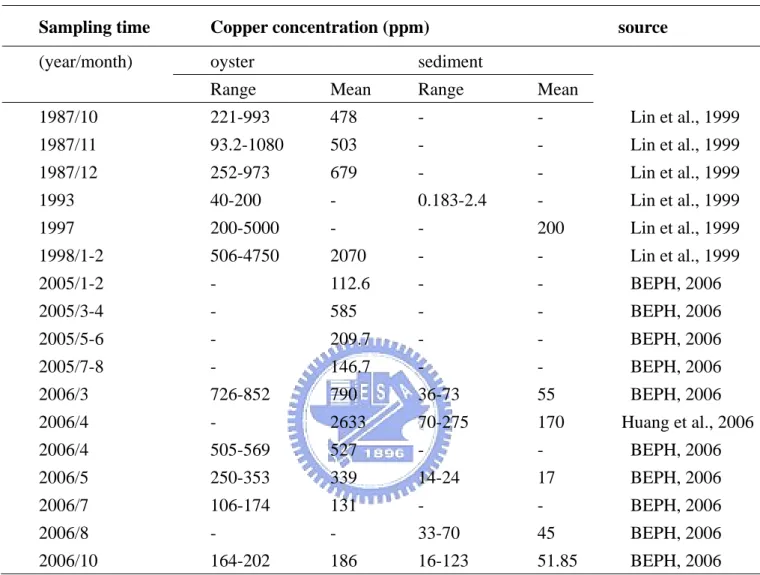
and sediments along the Hsianshan coastal area. Table 1 shows the statistics of the

copper concentrations of oyster and sediment in Hsianshan area sampled from 1987 to

2006. The table shows that the Hsianshan oyster had copper concentration with

average values ranging from 131 ppm to 790 ppm in the year from 1987 to 2006

except in 1998 which had an extremely high copper concentration of 2070 ppm.

Note that the copper concentrations reached 5000 ppm in 1997 and 4750 ppm in 1998

in some oyster samples. It is interesting to point out that the Cu concentration in

Siensan oyster has high Cu concentration in the winter and spring and low Cu

concentration in the summer, which is the rainy season in Taiwan. The reason for

this phenomenon may be attributed to the ingesting way of thin oysters in winter

(BEPH, 2006). In the wintertime of Taiwan, the sea sediment is disturbed by

(23)

heavy metal concentration mixed with the planktons are consumed by the oyster

through filtering ingestion. Long term ingestion of those substances with high Cu

concentration may result in a significant effect of bioaccumulation.

The regulation standards for Cu concentration in aquatic product are 100ppm and

30 ppm in Canada and Australia, respectively. Obviously, the problem of copper

pollution in Hsianshan oyster poses a serious threat to the local fishing community

and human health (Lin et al., 1999). Han et al. (1998) pointed out that the copper,

zinc, and arsenic concentrations in oysters were significantly higher than those in

other seafood in Taiwan. They also mentioned that those metals in the seafood

possibly comes from the wastewater discharged from various factories in the Keya

stream basin and the impact of metal pollution in the seafood and the health risk from

consuming the contaminated seafood desires public attention and further assessment

(Han et al., 1998).

1.4 Oysters character

There are a number of different groups of mollusks including oyster and shell which

grow in marine or brackish water. Some of these groups are highly prized as food,

both raw and cooked. Oysters are filter-feeders that draw water in over their gills

(24)

the mucus of the gills and transported to the mouth, where they are eaten, digested and

expelled as feces or pseudofeces. Feeding activity is greatest in oysters when water

temperatures are above 50°F (10°C). Healthy oysters consume algae and other

water-borne nutrients, each one filtering up to five litres of water per hour. Today

that feeding activity would happen almost a year. Nowadays, the sediment, nutrients,

and algae have contamination problems in local waters. Oysters filter these

pollutants, and either eat them or shape them into small packets that are deposited on

the bottom where they are harmless.

Oysters breathe much like fish, using both gills and mantle. The mantle is lined

with many small, thin-walled blood vessels which extract oxygen from the water and

expel carbon dioxide. A small, three-chambered heart, lying under the abductor

muscle, pumps colorless blood, with its supply of oxygen, to all parts of the body.

At the same time two kidneys located on the underside of the muscle purify the blood

of any waste products they have collected.

Heavy metal would accumulate in oyster organs. Oyster would get killed while a

abnomal water pollution occurred. The routes of copper into oyster organs divided

into two ways. The first way is that Cu in the seawater absorbed by algae, and then

(25)

directly ingests copper from seawater. In general, the appearance of greenish oyster

would happen while Cu concentration in oyster organs exceeds 500ppm.

1.5 Two green oyster investigation projects

Recently, there were two investigations in identifying the copper source for

Hsianshan green oyster. In April 2006, Huang et al. took water and sediment

samples from HSP and Keya stream for analyzing heavy metal concentrations (Huang

et al., 2006). In addition, they also measured the heavy metal concentrations in

oysters near Keya estuary for identifying the potential copper source in the Hsianshan

oyster. Table 2 shows the relative distance from the confluence of Nanman creek to

Keya stream or the locations of these 7 sampling points. The sampling point P is

inside the 2nd period of HSP for which the samples are pretreatment wastewater

mostly discharged from semiconductor manufacturing companies before entering the

wastewater treatment plant of HSP. The location of N0 is right at the discharge point

of the HSP at Nanman creek. The sampling point S is located at a municipal sewer

in the eastern part of Hsinchu city where the municipal wastewater is going to enter

the Keya stream. The sampling points Kd2 and Kd4 are located at Keya bridge and

Shiangya bridge, respectively, which are both at the downstream of the Keya stream.

(26)

from the downstream of the confluence of Nanman creek and Keya stream. The

sampling point I is at the intertidal zone of Keya stream. The sampling point C is at

the coastal area of Hsianshan. The water samples taken from those six sampling

points were analyzed for 18 heavy metals, including Zn, Cu, Pb, Fe, Al, Mn, Cd, Sr,

Cr, Ba, Ni, Ag, Sn, As, V, W, Ga, and Mo. The concentration data of those 18 heavy

metals, called as Data Set 1 given in (Huang et al., 2006), are graphed in Fig. 3,

showing that all the heavy metal concentrations are in ppb level and the Cu

concentrations sampled at P, N0, S, Kd2, Kd4, and I are 20, 340, 5, 15, 10, and 12 ppm,

respectively. The concentration data of Data Set 2 are graphed in Fig. 4, showing

that the Cu concentrations sampled at P, N0, S, Kd2, Kd4, I and C are 4600, 1400, 200,

500, 300, 250 and 100, respectively.

Huang et al. pointed out that the concentrations of Zn, Cu, Fe, Al, Sr, Ni, Cd, Sn, W,

Ga, and Mo at the N0, the discharge point of HSP, are higher than those at other

sampling points (Huang et al., 2006). Particularly, the Cu concentration at N0 is

several tens fold if compared with that at other sampling points, indicating that the

HSP is the Cu source for water in the downstream of Keya stream (Huang et al., 2006).

They also found very high concentrations of Zn, Cu, Pb, Fe, Al, Sr, Ba, Ni, W, and Ga

in the organs of oyster growing in the Hsianshan coast. In addition, the mean

(27)

are especially high among those 18 heavy metals. Note that the concentrations of Cu

in the sediment ranged from 70 to 275 ppm with an average of 170 ppm are also listed

in Table 1. They mentioned that the Cu source of oyster should relate to the high Cu

concentration discharged from HSP wastewater and the coastal sediment. In

addition to the Cu concentration, they also mentioned that the concentrations of Zn,

Fe, Al, Sr, Ni, W, and Ga are also high both in HSP wastewater and oyster, revealing

some relationship between the HSP wastewater and contaminated oyster. However,

they remarked that they did not have direct evidence to prove that that HSP is the

source of heavy metals of the Hsianshan wetland contamination (Huang et al., 2006).

An investigation was also conducted for identifying the copper source of Hsianshan

green oyster by the Bureau of Environmental Protection Hsinchu (BEPH) (2006).

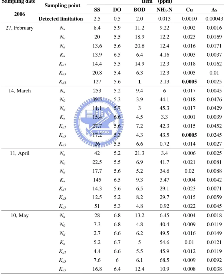
The water samples were collected at 7 sampling points, Nu, N0, Nd,Ku, Kd1, Kd3, and

Kd5 during the period of February to August, 2006 and analyzed for 6 chemical items

including SS, DO, BOD, NH3-N, Cu, As. One additional sampling point Y located at

Yuchegou creek was added and its water samples were taken from August to

November, 2006. The purpose of adding this sampling point is to assess whether the

HIP is a Cu source or not. The concentration data of those 6 chemical items for Data

Sets 3 to 12 respectively taken from February to November in 2006 are given in Table

(28)

is at Yuchegou creek, and Ku, Kd1, Kd3, Kd5 are at Keya stream. The sampling points

Nu and Nd are, respectively, located at the upstream and downstream of the discharge

point of HSP wastewater treatment plant at Nanman creek. The Ku is at the upstream

and Kd1, Kd3, Kd5 are at the downstream of the confluence of Nanman creek and Keya

stream. Table 2 shows the relative distances of those 8 sampling points measured

from the confluence of Nanman creek and Keya stream.

Most of the Cu concentrations in the sampling points listed in Table 3 are under the

environmental standard of 0.03 mg/L in the regulation for protecting human health

promulgated by Taiwan Environmental Protection Agency. The study of BEPH

pointed out that the Cu concentrations at N0 and Nd are relatively and equally high if

compared with those at Nu except in March and October, 2006. Table 3 shows that,

the concentration of Cu at Kd1, which is indeed located right at the downstream of N0

and Nd, is generally higher than those of other the downstream sampling points. It is

noticed that the Cu concentrations at Nu in March and October, at Ku in June and

October, and at Y in November are relatively high. However, there are no industrial

factories in the drainage basins located above the sampling points Nu and Ku. Those

data may be caused by illegal dumping of chemical wastes which happened

sometimes before in different rivers. The Cu concentration detected at Y reflects that

(29)

BEPH also mentioned that the Cu concentrations in oyster are higher in the winter and

spring and lower in the summer as indicated in Table 1. Note that this study also

estimates that the discharged Cu contained in the wastewater of the HSP to Nanman

creek is about 1263 kg/yr (BEPH, 2006).

1.6 Polytopic vector analysis

Polytopic vector analysis (PVA) is a hybrid of several algorithms developed over a

period of 30 years, primarily within the mathematical geology literature (Imbrie, 1963;

Miesch, 1976a; Miesch, 1976b; Klovan et al., 1976; Full et al., 1981; Full et al., 1982;

Ehrlich et al., 1987; Evans et al., 1992; Johnson, 1997). It is relatively new in the

environmental and chemometric area yet has been extensively used in the geological

sciences such as sedimentology, petrophysics, and igneous petrology. The formalism

of the PVA algorithm is outlined in detail by Johnson (1997). The PVA is

self-training method used to determine the three parameters of interest in a mixed

system: (1) the number of end-members; (2) the chemical composition of each

end-member (in percent); and (3) the relative contribution of each end-member in

each sample (in percent) (Johnson et al., 2002).

Johnson et al. (2000) used PVA to resolve a source degradation model developed

(30)

Estuary, California. Chemical fingerprints were identified related to known

industrial formulations of PCB mixtures, as well as to natural degradation processes

of the original PCB source profiles. Barabas (2004a, b) et al. developed a modified

algorithm (M-PVA) to resolve a dioxin dechlorination fingerprint, indicative of

biotic/abiotic transformations in field samples of sediments. Bright et al. (1999)

used PVA to apportion sources of dioxins and furans to Howe Sound and the lower

Strait of Georgia marine ecosystem, British Columbia, Canada, based on the

deposition in recent sediments. DeCaprio et al. (2005) used PVA to determine the

number, composition, and relative proportions of independent congener patterns that

contributed to the overall serum PCB profile. Huntley et al. (1998) utilized PVA to

determine the number of dominant fingerprint patterns of sediment cores collected

throughout the Newark Bay Estuary and analyzed for polychlorinated

dibenzo-p-dioxins and dibenzofurans (PCDD/Fs). The PVA results indicated that

comparison of end-member patterns with source-specific fingerprint patterns found

three PCDD/F congener patterns common to all models: combustion source, sewage

sludge sources, and sources associated with polychlorinated biphenyls (PCBs).

PVA was performed in two steps. The first is a principal components analysis

performed on the transformed matrix. Evaluation of the number of significant

(31)

done using the goodness-of-fit criteria of Miesch (1976) and Johnson (1997). The

second step in PVA determines the chemical composition of the end-member sand

and the relative proportions of each end-member in each sample. This step uses the

DENEG algorithm of Full et al. (1981, 1982).

1.7 Objectives

The problem of green oyster in Hsianshan wetland results in several ten million (in

US dollars) loss in the fishery, and draws a lot of attention from public and

government in Taiwan. Several studies had been made (BEPH, 2006; Lin et al.,

1999; Huang et al., 2006) in identifying the copper source of green oyster incidents,

yet, no persuasive result or clear evidence points out the source of the copper so far.

Therefore, the objective of this thesis is to identify the source of copper in green

oyster which has been a serious and unsolved problem in the past two decades. Note

that in the summer and autumn, i.e., the rainy seasons in Hsinchu; the river stage is

high and the contaminant concentration in water samples were diluted by the large

amount of stream water. Therefore, we utilize PVA to analyze 12 data sets taken in

April, 2006 from (Huang et al., 2006) and in February to November, 2006 (BEPH,

(32)

CHAPTER 2 MATERIAL AND METHOD

2.1 PVA Formalism

This section presents the full PVA algorithm running under default conditions; that

is (1) the Q-mode factor analysis algorithm originally presented as the Fortran IV

program EXTENDED CABFAC (Klovan and Miesch, 1976) and (2) the iterative

oblique vector rotation algorithm originally presented as the Fortran IV program

EXTENDED QMODEL (Full et al. 1981). While any number of alternative data

transformation and calculation options are available and are often implemented, these

algorithms represent the core of PVA as it is presently implemented under default

options by the commercial version of the Quick Start software system.

2.2 Matrix adjustments

Prior to applying the PVA algorithm, several matrix adjustments to the data are

required. The sampled concentrations in the Data Sets 1 and 2 are all greater than

the detection limits; therefore, no adjustment is needed. However, the matrix of the

Data Sets 3 to 12 contains a number of data where their concentrations are below the

detection limits. In order to have a robust data set for the statistical analysis, the

(33)

of the reported detection limits.

Three data transformations are performed. First, the data are normalized as

constant row-sum sample vectors (i.e., concentrations are expressed as percent of total

concentration). Then the range transformation is applied to all the variables such

that their values fall in the range from 0 to 1. Finally, each of the sample vectors is

transformed to having equal Euclidean length (Miesch, 1976).

2.3 Polytopic Vector Analysis

In this study, the PVA of “Quick start” package is used for the analyses. The

“Quick start” is a shorter version of the manual using the most likely default values

for PVA. The software was written based on the original algorithms of Klovan and

Miesch (1976) and Full et al. (1981). The full PVA algorithm running under default

conditions; that is (1) the Q-mode factor analysis algorithm originally presented as the

Fortran IV program EXTENDED CABFAC (Klovan and Miesch, 1976) and (2) the

iterative oblique vector rotation algorithm originally presented as the Fortran IV

program EXTENDED QMODEL (Full et al., 1981).

The objective of PVA is to resolve three parameters of concern in a mix system: (1)

the number of components (termed end-members) in the mixture, (2) the identity (i.e.,

(34)

end-member in each sample. To state the problem mathematically, given a matrix X

of m samples and n variables, and the true (but as yet unknown) number of

end-members k, a feasible solution may be found and expressed as:

X = A F (m n× ) (m k× ) (k n× )

(1)

where A is a matrix of mixing proportions (the relative proportions of each of k

end-members in each sample), and F is a matrix of k end-member compositions.

The PVA is performed in two steps. The Klovan and Miesch (1976) algorithm is

used to determine the number of end-members (k end-members). The number of

significant eigenvectors is equal to the number of end-members in the model, and is

evaluated using (1) normalized varimax loadings of Klovan and Miesch (1976) and (2)

the coefficient of determination (CD) of Miesch (1976) and the CD scatter plots of

Johnson (1997). The second step in PVA modeling involves an iterative algorithm

(Full et al., 1981) that determines the chemical composition of the end-members and

the relative proportions of each end-member in each sample.

2.4 Determining the number of end-members

Of the many varieties of eigenvector methods, no topic has created more argument

and controversy than the criteria used to determine the correct number of eigenvectors

(i.e., k: the number of factors, or end-members). In this section, a number of

(35)

presented, and a graphical method is proposed.

2.4.1 Average Eigenvalue Criterion

This criterion is based on the rationale that only those principal components whose

eigenvalues are above the average eigenvalue should be retained for the model. This

criterion was first propose be Kaiser (1960). In those cases where principal

components analysis (PCA) is performed index on the correlation matrix, the average

eigenvalue will be 1.0. As such, this index is also referred to as the eigenvalue-one

criterion (Malinowski, 1991).

2.4.2 Cumulative Present Variance

The rationale for this criterion is simple: a large percentage of the variance in the

original matrix should be accounted for by a reduced dimensional model. However,

workers in multivariable statistics, chemometrics and mathematical geology generally

acknowledge that any proposed cutoff criterion is arbitrary (Deane, 1992; Reyment

and Joreskog, 1993; Malinowski, 1991). The lack of a clear criterion makes the

cumulative variance method dubious.

2.4.3 Scree Test

The scree test of Cattel (1966) is based on the supposition that the residual

(36)

point where the principal components begin accounting for number, the point where

the curve begins to level off should show a noticeable inflection point, or “knee”.

2.4.4 Normalized Varimax Loadings

The factor analysis program of Klovan and Miesch (1976) included a subroutine

that calculate the number of samples with normalized varimax factor loadings greater

than 0.1. The analyst looks for a sharp drop in the index as an indication of the

appropriate number of eigenvectors.

2.4.5 The coefficient of determination (CD) and the CD scatter plots

Given an m sample by n variable data matrix X the index used by Miesch (1976)

was the “coefficient of determination” (CD) between each variable in the original data

matrix (X) and its back-calculated reduced dimensional equivalent ( ˆX ). For each number of potential eigenvectors, 1, 2 …n, Miesch calculated a n×1 vector as:

2 2 2 2 ( ) ( ) ( ) j j j j s x d r s x − ≅ (2)

where s(x)j2 is the variance in the jth column of X and (dj)2 is the variance of residuals

between column j of X and column j of ˆX . The Miesch CD is the r2 with respect to

a line of one-to-one back-calculation between Xj and ˆXj.

A graphical extension of Miesch’s method has recently been implemented by

(37)

the fit of the Miesch CD is a series of n scatter plots that show the measured value for

each variable Xj plotted against the back-calculated values from the k proposed

(38)

CHAPTER 3 RESULTS AND DISCUSSION

3.1 PVA results based on Huang et al.’s data

3.1.1 The chemical pattern of Data Set 1

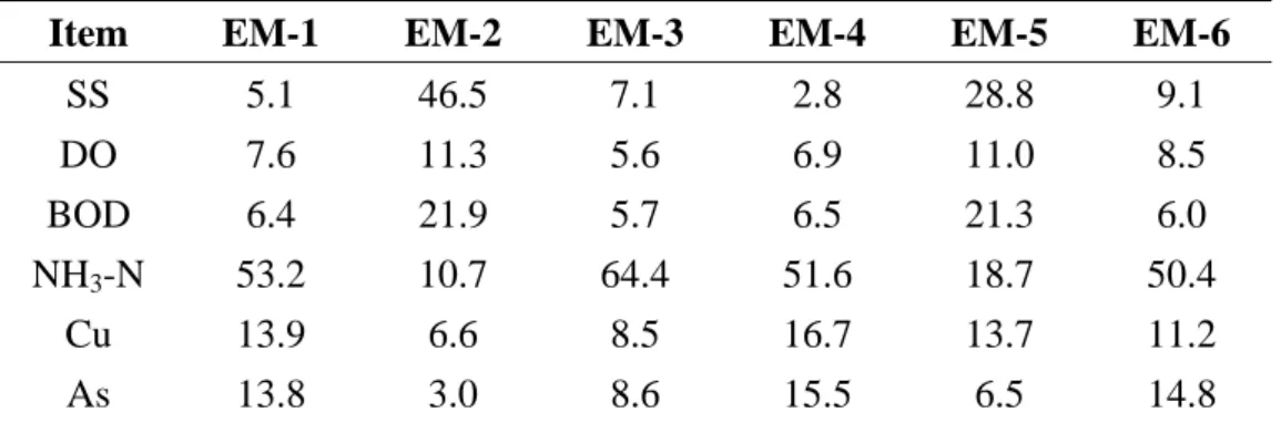
The chemical composition and geographic distribution of each end-member (EM)

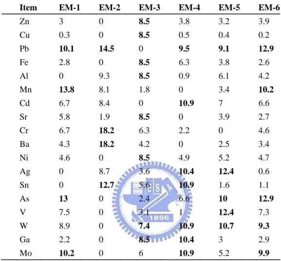
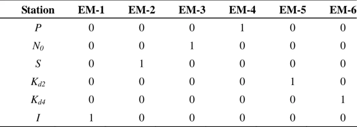
obtained from Data Set 1 for water samples are shown in Tables 5 and 6, respectively.

Table 5 presents the end-member fingerprint compositions (in percent) analyzed

through PVA of 6×18 data matrix with a 6 end-member model. Table 6 shows the

end-member fingerprint compositions (in decimal percentages) analyzed through PVA

with the same data matrix and end-member model as the previous one.

EM-1 represents the chemical fingerprint in the sampling point I which is located at

the intertidal zone of Keya stream. It is characterized by high proportions of Pb

(10.1%), Mn (13.8%), As (13%), and Mo (10.2%). EM-2 represents the fingerprint

in S for the municipal sewer in the eastern part of Hsinchu city with high proportions

of Pb(14.5%), Cr(18.2%), Ba(18.2%), and Sn(12.7%). Those heavy metals in the

municipal wastewater may be from some factories such as electroplating plant or steel

plant in the city. EM-3 stands for the HSP wastewater (N0) fingerprint, characterized

(39)

W(7.4%), and Ga(8.5%). EM-4 represents the fingerprint at P (2nd period of HSP),

characterized by Pb(9.5%), Cd(10.9%), Ag(10.4%), Sn(10.9%), W(10.9%),

Ga(10.4%), and Mo(10.9%). EM-5 represents the fingerprint at Kd2 (Keya Bridge),

characterized by Pb(9.1%), Ag(12.4%), As(10.0%), V(12.4%), and W(10.7%).

EM-6 represents the chemical fingerprint at Kd4 (Shiangya Bridge), characterized by

Pb(12.9%), Mn(10.2%), As(12.9%), W(9.3%), and Mo(9.9%).

Huang et al. (2006) mentioned that the high concentrations of heavy metals,

including Zn, Cu, Pb, Fe, Al, Sr, Ba, Ni, W, and Ga, in the organs of oysters were

found along the Hsianshan coast. From PVA results, EM-3 represents the HSP

wastewater fingerprint characterized by high proportions of Zn, Cu, Fe, Al, Sr, Ni, W,

and Ga. These results strongly support the conclusion that the heavy metals in oyster

organs were mainly from the wastewater of HSP. In addition, EM-2 is characterized

by high proportions of Pb, Cr, Ba, and Sn. Accordingly, the source of Pb and Ba in

oyster organs may come from the municipal wastewater sewer. On the other hand,

the heavy metals of the other EMs are recovered from a small number of the factories

distributed in the Hsinchu city.

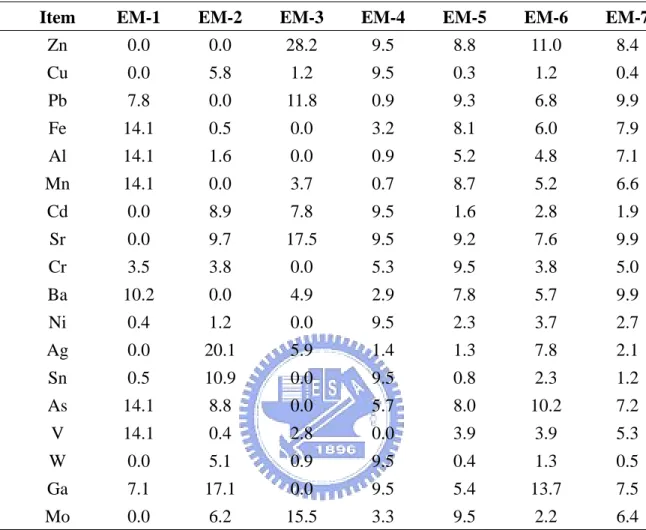
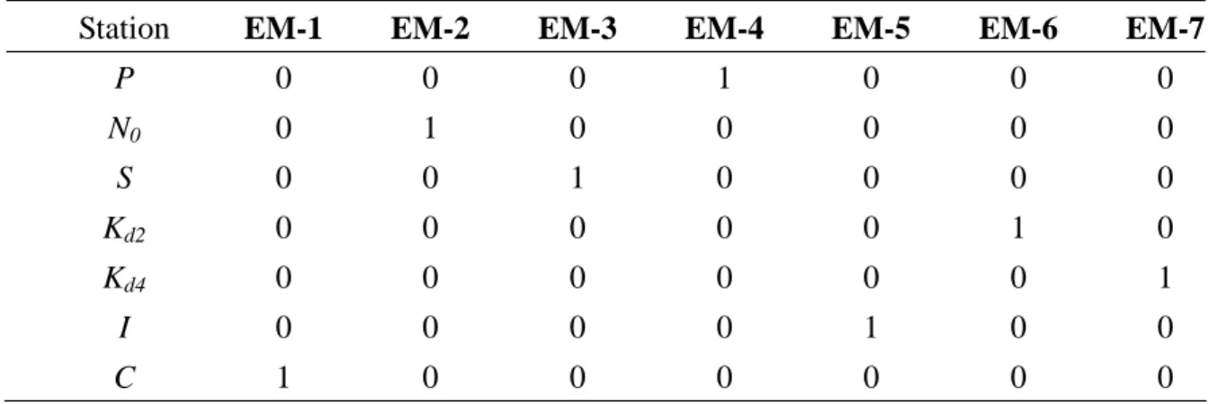
3.1.2 The chemical pattern of Data Set 2

(40)

distribution of each end-member (EM) obtained from Data Set 2 for suspended solid

samples. Table 7 presents the end-member fingerprint compositions (in percent)

analyzed through PVA of 7×18 data matrix with a 6 end-member model. Table 8

shows the end-member fingerprint compositions (in decimal percentages) analyzed

through PVA with the same data matrix and end-member model as the previous one.

EM-1 represents the chemical fingerprint in the sampling point C which is located

at the coastal area of Hsianshan. It is characterized by high proportions of

Fe(14.1%), Al(14.1%), Mn(14.1%), Ba(10.2%), As(14.1%) and V(14.1%). EM-2

represents the fingerprint for the HSP wastewater discharge point (N0) with high

proportions of Ag(20.1%), Sn(10.9%), Ga(17.1%) and a relative high proportion

Cu(5.8%) compared with other end-members. EM-3 stands for S representing the

municipal sewer in the eastern part of Hsinchu city with high proportions of

Zn(28.2%), Pb(11.8%), Sr(17.5%) and Mo(15.5%). EM-4 represents the fingerprint

at P (2nd period of HSP), characterized by Zn(9.5%), Cu(9.5%), Cd(9.5%), Sr(9.5%),

Ni(9.5%), Sn(9.5%), W(9.5%) and Ga(9.5%). EM-5 represents the fingerprint at I,

which is located at the intertidal zone of Keya stream, with high proportions of

Zn(8.8%), Pb(9.3%), Fe(8.1%), Mn(8.7%), Sr(9.2%), Cr(9.5%), As(8.0%) and

Mo(9.5%). EM-6 represents the chemical fingerprint at Kd2 (Keya Bridge),

(41)

chemical fingerprint at Kd4 (Shiangya Bridge), characterized by Zn(8.4%), Pb(9.9%),

Sr(9.9%), and Ba(9.9%).

Relative high Cu proportions with 5.8% and 9.4% in EM-2 and EM-4, respectively,

can be observed. EM-2 represents the HSP wastewater fingerprint and EM-4

represents the fingerprint at P (2nd period of HSP).

3.2 On the PVA results from Data Sets 1 and 2

Results from both the water samples and suspended solid samples indicate that high

Cu proportion appearing from the HSP discharge point into the Keya stream. In

addition, the PVA results of Data Set 1 show that eight heavy metals concentrations

are high in both HSP wastewater point and oyster organs. Based on these results, it

is reasonable to conclude that the HSP is a major Cu source to the green oyster.

3.3 PVA results for the data from BEPH project

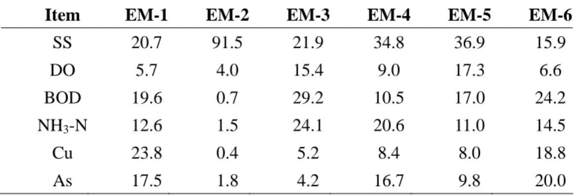
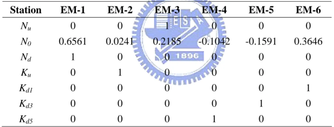
3.3.1 The chemical pattern of Data Set 3

Data Sets 3 to 12 are water samples collected from Keya stream, Nanman creek,

and Yuchegou creek. The chemical composition and geographic distribution of each

(42)

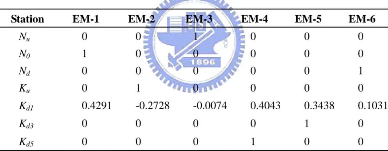
10, respectively. Table 9 represents the end-member fingerprint compositions (in

percent) analyzed through PVA of 7×6 data matrix with the 6 end-member model.

Table 10 is the end-member fingerprint compositions (in decimal percentages)

analyzed through PVA from the same data matrix and end-member model. EM-3

represents the chemical pattern for samples taken from Nu. It is characterized by

high proportions of SS (21.9%), BOD (29.2%) and NH3-N (24.1%). The pattern in

N0 is characterized by EM-1 with high proportions of Cu (23.8%), SS (20.7%) and

BOD (19.6%). EM-6 represents the chemical pattern for Nd, characterized by BOD

(24.2%), Cu (18.8%) and As (20.0%). This conforms that the metal, Cu, comes from

the discharge point of HSP (N0) and contributes to it downstream point Nd.

EM-5 represents the fingerprint for Ku, characterized by high proportions of SS

(36.9%), BOD (17.0%) and DO (17.3%). Note that the proportion of Cu in EM-2 is

only 8.0%. It indicates that the major copper source may not be from the upstream

reach of Keya stream (Ku). The pattern represents for Kd1 is EM-1 and EM-4. The

proportion of copper is obviously high in EM-1 and EM-6, characterized by 23.8%

and 8.4%, respectively. The result indicates that Kd1 has high Cu proportion

originated from the Nanman creek. In other words, the Cu in Kd1 also comes from

the HSP discharge point. However, there are low copper proportions in Kd3 and Kd5

(43)

discharged from municipal sewers and Yuchegou creek.

3.3.2 The chemical pattern of Data Set 4

Table 11 and Table 12 respectively the chemical composition and geographic

distribution of each end-member (EM) of Data Set 4 obtained from PVA are shown in.

Table 11 represents the end-member fingerprint compositions (in percent) analyzed

through PVA of 7×6 data matrix with the 6 end-member model. Table 12 is the

from the same data matrix and end-member model. EM-3 represents the chemical

pattern for samples taken from Nu. It is characterized by high proportions of SS

(85.7%). The pattern represents for N0 is EM-1 and EM-6. The proportion of

copper is obviously high in EM-1 and EM-6, characterized by 13.6% and 10.5%,

respectively. EM-1 represents the chemical pattern for Nd, characterized by NH3-N

(36.2%), Cu (13.6%) and As (34.3%). This conforms that the metal, Cu, comes from

(44.4%), BOD (13.0%) and As (11.2%). Note that the proportion of Cu in EM-2 is

only 2.9%. It indicates that the major copper source is not from the upstream reach

(44)

proportions of NH3-N (29.6%), Cu (10.5%) and As (31.6%). The result indicates

that Kd1 has high Cu proportion originated from the Nanman creek. In other words,

the Cu in Kd1 also comes from the HSP discharge point. Similarly, the copper

proportion in Kd5 is high (25.2%). Yet, the Cu proportions in Kd3 is low which may

be diluted by large amount of wastewater discharged from municipal sewers and

Yuchegou creek.

3.3.3 The chemical pattern of Data Set 5

Table 13 and Table 14 respectively represent the chemical composition and

geographic distribution of each end-member (EM) of Data Set 5 obtained from PVA.

(52.2%) and BOD (26.5%). The pattern represents for N0 is EM-1. The proportion

of copper is obviously high, characterized by 19.9% in EM-1 revealing that the Cu

may come from the HSP. EM-6 represents the chemical pattern for Nd, characterized

(45)

(84.1%). Note that the proportion of Cu in EM-2 is only 2.3%. It indicates that the

major copper source is not from the upstream reach of Keya stream (Ku). The

pattern in Kd1 is comprised by EM-1 with 42.9% and EM-4 with 40.4%, the

proportions of Cu in EM-1 and EM-4 are 19.9% and 24.9%, respectively. The result

indicates that Kd1 has high Cu proportion originated from the Nanman creek. In

other words, the Cu in Kd1 also comes from the HSP discharge point. Similarly, the

high copper proportions in Kd3 and Kd5 are 19.6% and 24.9%, respectively. We are,

therefore, reasonably to conclude that the copper found at Kd3 and Kd5 located at the

downstream reaches of Keya River comes from the HSP discharge point.

3.3.4 The chemical pattern of Data Set 6

of Data Set 6 obtained from PVA are respectively shown in Table 15 and Table 16.

through PVA of 7×6 data matrix with the 6 end-member model. Table 16 lists the

(46)

pattern for samples taken from Nu characterized by high proportions of SS (46.5%)

and BOD (21.9%). The pattern represents for N0 is EM-6. The proportion of

copper is relative high, characterized by 11.2% in EM-6 revealing that the Cu may

also come from the HSP. EM-4 represents the chemical pattern for Nd, characterized

by NH3-N (51.6%) and Cu (16.7%). Table 15 also shows that the proportions of

NH3-N are higher than 50% in EM-1, EM-3, EM-4, and EM-6. Those analyzed

results reflect that both Cu and NH3-N come from the discharge point of HSP (N0) and

contributes to its downstream sampling points.

The pattern in Ku is comprised by EM-3 with 45.5% and EM-6 with 69.4%, the

proportions of Cu in EM-1 and EM-4 are 8.5% and 11.2%, respectively. It indicates

that the major copper source is not from the upstream reach of Keya stream (Ku).

The pattern in Kd1 is characterized by EM-1 with high proportion of NH3-N (53.2%)

and Cu (13.9%). The result indicates that Kd1 has high Cu proportion originated

from the Nanman creek. In other words, the Cu in Kd1 also comes from the HSP

discharge point. Similarly, the copper proportion in Kd5 is 13.7%. However, the Cu

proportion in Kd3 is 8.5% which may reflect the problem of dilution. We are,

therefore, reasonably to conclude that the copper found at Kd3 and Kd5 located at the

(47)

3.3.5 The chemical pattern of Data Set 7

of Data Set 7 obtained from PVA are shown in Table 17 and Table 18, respectively.

(34.7%) and DO (24.9%). The pattern represents for N0 is EM-5 which has a high

proportion of copper, characterized by 15.9% in EM-5. EM-2 represents the

chemical pattern for Nd, characterized by SS (87.4%).

The pattern in Ku is characterized by EM-6 with high proportion of NH3-N (38.1%),

As (34.0%) and Cu (13.8%). The pattern in Kd1 is characterized by EM-1 with high

proportion of NH3-N (42.2%), As (22.5%) and Cu (16.7%). The pattern in Kd3 is

comprised by EM-2 with 75.2% and EM-6 with 90.1%, the proportions of Cu in

EM-1 and EM-4 are 4.1% and 13.8%, respectively. The pattern in Kd5 is

characterized by EM-3 with high proportion of SS (70.2%) and Cu (18.2%).

(48)

rainfall record shown in Fig. 5 indicates that it were the rainy days from 28 to 31, May

and 2 to 4, June. This is the reason why the proportions of SS at sampling points are

very high in the sampling points of EM-2 and EM-3. It is difficult to observe the

trend of Cu proportion based on the result of PVA for Data. Table 3 shows the

original copper data taken in July, 2006 from various sampling points. The Cu

concentrations have the same order of magnitude for N0 and Nd at Nanman creek and

for Ku, Kd1, and Kd5 are at Keya stream. This fact indicates that N0 is one of the Cu

source to its downstream sampling points.

3.3.6 The chemical pattern of Data Set 8

Table 19 and Table 20 respectively show the chemical composition and geographic

distribution of each end-member (EM) of Data Set 8 obtained from PVA. Table 19

represents the end-member fingerprint compositions (in percent) analyzed through

PVA of 7×6 data matrix with the 6 end-member model. Table 20 is the end-member

fingerprint compositions (in decimal percentages) analyzed through PVA from the

same data matrix and end-member model. EM-3 represents the chemical pattern for

samples taken from Nu. It is characterized by high proportions of SS (53.3%). The

pattern in N0 is major characterized by EM-6 with 83.5%, the proportions of Cu in

(49)

concentration. EM-6 represents the chemical pattern for Nd, characterized by Cu

(40.6%). This conforms that the metal, Cu, comes from the discharge point of HSP

(N0) and contributes to it downstream point Nd.

EM-5 represents the chemical pattern for samples taken from Ku. It is

characterized by high proportions of SS (45.5%). It indicates that the major copper

source is not from the upstream reach of Keya stream (Ku). The pattern in Kd1 is

characterized by EM-1 with high proportion of Cu (36.9%) and SS (19.7%). This

result indicates that Kd1 has high Cu proportion originated from the Nanman creek.

In other words, the Cu in Kd1 also comes from the HSP discharge point. Similarly,

the high copper proportion in Kd3 and Kd5 are 21.6% and 17.3%, respectively.

Therefore, it is reasonably to conclude that the copper found at Kd3 and Kd5 located at

the downstream reaches of Keya River comes from the HSP discharge point.

3.3.7 The chemical pattern of Data Set 9

distribution of each end-member (EM) of Data Set 9 obtained from PVA. The

end-member fingerprint compositions (in percent) analyzed through PVA of 8×6 data

matrix with the 6 end-member model are listed in Table 21. Table 22 is the

(50)

(33.5%), DO (18.3%) and BOD (18.6%). The pattern in N0 is major characterized

by EM-1 (75.6%) and EM-3 (41.8%) with the proportions of Cu in EM-1 is 5.4 % and

in EM-3 is 6.3%. EM-6 represents the chemical pattern for Nd, characterized by Cu

(46.8%).

characterized by high proportions of NH3-N (36.2%) and As (34.4%). It indicates

that the major copper source is not from the upstream reach of Keya stream (Ku).

The pattern in Kd1 mainly consists of EM-1 and EM-6 with Cu proportion of 5.4% and

46.8%, respectively. Similarly, the copper proportion in Kd3 and Kd5 are 6.3% and

10.1%, respectively. EM-4 represents the chemical pattern for the sample collected

from Y. It is characterized by high proportion of SS (20.2%), DO (24.5%) and BOD

(22.7%). Accordingly, it is to conclude that the copper found at Kd3 and Kd5 located

at the downstream reach of Keya River come from the sampling points of Nd and Kd1

and, very likely, also come from HSP discharge point.

3.3.8 The chemical pattern of Data Set 10

(51)

The end-member fingerprint compositions (in percent) analyzed through PVA of 8×6

data matrix with the 6 end-member model is shown in Table 23. Table 24 is the

from the same data matrix and end-member model. Note that this data set was

sampled in Sept. 12 and Sept. 8 to 12 were rainy days according to the rainfall record

shown in Fig. 5. The proportions of Cu shown in Table 23 are very low for all the

sampling points except Kd5 and Y indicating that Y may be a minor copper source.

3.3.9 The chemical pattern of Data Set 11

from the same data matrix and end-member model.

Nu is mainly composed by EM-5 (55.2%) and EM-6 (65.4%). EM-5 is major

characterized by NH3-N (56.6%) and Cu (16.2%). EM-6 is major characterized by

(52)

high proportions of As (42.9%) and SS (15.4%). EM-5 represents the chemical

pattern for Nd, characterized by NH3-N (56.6%).

characterized by high proportions of SS (33.5%) and Cu (33.9%). The pattern in Kd1

is mainly composed by EM-5 and EM-6 with Cu proportion of 16.2% and 21.9%,

respectively. Similarly, the copper proportion in Kd3, Y, and Kd5 are 21.9%, 26.5%,

and 13.5%, respectively. Therefore, the results indicate that the copper found at Kd1,

Kd3 and Kd5 mainly comes from upstream of Nanman creek and upstream of Keya

stream.

3.3.10 The chemical pattern of Data Set 12

distribution of each end-member (EM) of Data Set 12 obtained from PVA. Table 27

represents the end-member fingerprint compositions (in percent) analyzed through

PVA of 8×6 data matrix with the 6 end-member model. Table 28 is the end-member

fingerprint compositions (in decimal percentages) analyzed through PVA from the

same data matrix and end-member model.

(53)

mainly represented by EM-1 (285.6%). EM-1 is major characterized by NH3-N

(42.4%) and As (38.2%). EM-6 represents the chemical pattern for Nd, characterized

by NH3-N (39.3%) and As (42.7%).

characterized by high proportions of SS (45.8%) and Cu (20.3%). EM-1 represents

the chemical pattern for samples taken from Kd1. It is characterized by high

proportions of NH3-N (42.4%) and As (38.2%). The pattern in Kd3 is composed by

EM-1 and EM-4 with Cu proportion of 5.9% and 20.3%, respectively. There is a

high copper proportion in Y with 71.0%. The pattern in Kd5 is characterized by

EM-5 with high proportions of SS (41.6%) and Cu (19.2%). Therefore, it is to

conclude that the copper found at Kd5 located at the downstream may mainly comes

from Youchegou creek (Y).

3.4 On the PVA results from Data Sets 3 to 12

From PVA results of Data Sets 3 to 9, it appears that high or relatively high

proportion of copper can be found at N0 and most of its downstream sampling points

Nd, Kd1, Kd3, and Kd5. This result also supports the finding that the source of copper

comes from the discharge point of wastewater from the HSP.

應用多方向量分析分析污染檢測數據

國 立 交 通 大 學

環 境 工 程 研 究 所

碩 士 論 文

應 用 多 方 向 量 分 析 分 析 污 染 檢 測 數 據

The Analyses of Sampling Data Using

Polytopic Vector Analysis

研 究 生：莊 敏 筠

指導教授：葉 弘 德 教授

應 用 多 方 向 量 分 析 分 析 污 染 檢 測 數 據

The Analyses of Sampling Data Using

Polytopic Vector Analysis

研 究 生 ： 莊敏筠

Student：Min-Yun Chuang

指導教授： 葉弘德

Advisor：Hund-Der Yeh

國 立 交 通 大 學

環 境 工 程 研 究 所

碩 士 論 文

A Thesis

Submitted to Institute of Environmental Engineering

College of Engineering

National Chiao Tung University

in Partial Fulfillment of the Requirements

for the Degree of

Master of Science

in

Environmental Engineering

August, 2007

Hsinchu, Taiwan

中 華 民 國 九 十 六 年 八 月

應 用 多 方 向 量 分 析 分 析 污 染 檢 測 數 據

研究生：莊敏筠 指導教授：葉弘德

國立交通大學環境工程研究所

摘 要

鑒定化學污染源與瞭解污染團在時空上的分佈，在環境污染領域

是重要且新受矚目的問題。在多重污染源地區，環境工程師面臨著如

何鑒定複雜地形的污染源型態。如果污染源具有獨特的化學指紋，即

可藉由多變數統計分析方法來進一步解決環境指紋問題。

多方向量分析(Polytopic Vector Analysis)是一種鑑定污染源化學

指紋的多變量分析統計方法。假定某一混合系統，多方向量分析可用

來計算三個重要參量：(1)來源(後端成分)個數、(2)各後端成分的化學

指紋組成、以及(3)不同樣本中來自各來源的濃度相關比例。

本研究應用多方向量分析，分別針對兩個研究案例做分析(I)客雅

溪流域重金屬檢測數據，以及(II)新竹科學園區地下水有機污染檢測

資料。

近年來，在新竹香山海域養殖的牡蠣及沈積物的銅含量皆出現顯

著增高的趨勢。綠牡蠣體內伴隨著高濃度的銅含量，不但威脅消費者

健康且影響漁民每年三百多萬美金產值。香山牡蠣銅污染的來源是長

久被關切且極需解決的問題。雖然在過去的研究曾指出香山海域銅污

染可能源自於新竹科學園區或香山工業區，然而卻缺少強而有力的證

據指出確切的污染者。於 2006 年檢測客雅溪及其支流的十二組數

據，這十二組數據分別來自於不同兩組研究團隊的檢測成果。本研究

目的在於利用統計方法-多方向量分析，鑑定綠牡蠣組織內的重金屬

銅之來源。第一組及第二組數據，分別在客雅溪沿岸檢測共 6 個水樣

及 7 個懸浮固體樣本，採樣時間為 2006 年四月，每個取樣分析 18 種

重金屬項目(鋅、銅、鉛、鐵、鋁、錳、鎘、鍶、鉻、鋇、鎳、銀、

錫、砷、釩、鎢、鎵及鉬)。第三組到第八組數據，沿客雅溪流域 7

個取樣點，採樣時間為 2006 年二月至七月；第九組到第十二組數據，

沿客雅溪流域 8 個取樣點，採樣時間於 2006 年八月至十一月，每個

水樣分析六個項目(懸浮固體、溶氧、生化需氧量、氨氮、銅及砷)。

由多方向量分析結果顯示，新竹科學園區為綠牡蠣中銅的主要來源。

在第二個研究案例，係應用多方向量分析針對新竹科學園區地下

水污染檢測資料作分析，利用計算係數以及因子負荷係數判定該工業

區地下水有機污染物資料，鑒定出有六個有機污染物指紋，進而計算

出各後端成分在地理上的分佈。因此，利用多方向量分析可決定後端

成分的個數，並且發展出一個地下水污染物的混合模式，以模擬地下

水污染源化學指紋與污染團在空間上的分佈。

The analyses of sampling data using

Polytopic vector analysis

Student: Min-Yun Chuang Advisor: Hund-Der Yeh

Institute of Environmental Engineering

National Chiao Tung University

ABSTRACT

致謝

TABLE OF CONTENTS

摘 要 ... I

ABSTRACT... III

致謝...VII

TABLE OF CONTENTS... VIII

國立交通大學

環境工程研究所

碩士論文

應用多方向量分析分析污染檢測數據

研究生：莊敏筠

指導教授：葉弘德教授

應用多方向量分析分析污染檢測數據

研究生：莊敏筠

指導教授：葉弘德

國立交通大學

環境工程研究所

碩士論文

中華民國九十六年八月

應用多方向量分析分析污染檢測數據

研究生：莊敏筠指導教授：葉弘德

摘要

摘要 ... I