A New Multi-Stage Weighted Interference Cancellation Multiuser Detector With
User Ordering for DS-CDMA
Chen-Chu Hsu Yumin Lee
Graduate Institute of Comm. Eng. AndDept. of Electrical Eng., National Taiwan University
Taipei 10617, Taiwan
TEL: +886-2-23626508 FAX: +886-2-23683824 E-mail: [email protected]
Abstract – Conventional multi-stage multi-user detectors
(MUD) such as the parallel interference cancellation (PIC) MUD suffer from error propagation. In this paper, we propose a new multi-stage MUD in which reliability weighting factors are applied to reduce error propagation. An algorithm is derived for optimizing both the reliability weighting factors and decision order for the proposed structure. Simulation results show that the proposed MUD almost achieves the single user bound with just a few stages.
I. INTRODUCTION
Multiple access interference (MAI) is a dominant capacity-limiting of multiuser communication systems based on direct-sequence code division multiple access (DS-CDMA). In a conventional DS-CDMA receiver, detection of the desired user’s signal is performed while treating MAI as thermal noise. Although simple in structure, the conventional receiver fails to realize the full potentials of DS-CDMA because treating MAI as noise loses much information about the structure of MAI. Significant improvement over the conventional receiver can be achieved by viewing MAI as signal rather than thermal noise, and jointly detecting all users’ information symbols. This improved detector is referred to as the multi-user detector (MUD) in the literature[1].
Many MUD structures can be found in the literature for different applications and channel conditions. The interference cancellation MUD [1,4] is one of the most suitable choices for quasi-synchronous uplink DS-CDMA transmission over flat fading channels. In an interference cancellation MUD, MAI is estimated and then subtracted from the received signal. Parallel interference cancellation (PIC) and successive interference cancellation (SIC) MUDs are two common examples of this MUD. PIC first estimates the MAI and then subtracts them from the received signal in parallel. If the estimated MAI is perfect, then the MAI will be completely removed from the received signal. Unfortunately, the MAI estimate is inevitably noisy. When the estimate is in error, MAI can potentially be strengthened, instead of cancelled, by the action of PIC. Partial PIC [2,7,8,9] is one method for
alleviating this problem. In PPIC, MAI estimates are scaled before being subtracted from the received signal using weightings that are empirically determined, thus reducing the sensitivity to errors in the estimated MAI. Since the weightings are obtained by trial-and-error, dynamically adjusting the weightings can be costly.
In this paper, we propose a new multi-stage MUD, referred to as the nonparallelizable weighted interference cancellation MUD, that is a novel generalizations of PPIC. A new algorithm is also proposed to jointly optimize the user decision order and reliability weighting factors for MAI estimations. Simulation results show that significant improvement is achievable by the proposed algorithm. In fact, the proposed MUD almost achieves the performance of single user (SU) bound with a few stages.
II. SYSTEM MODEL
Consider a synchronous DS-CDMA system in which
K≥1 active users transmit their data streams simultaneously over wireless flat-fading channels. The baseband equivalent received signal is expressed as
∑ ∑
= + − = K k k m k k d mg t mT nt A t r 1 ) ( ) ( ] [ ) ( , (1)where A ,k gk(t) , and dk[m] are, respectively, the flat-fading channel gain, signature waveform, and m-th modulation symbol of the k-th user, T is the symbol-period, and n(t) is the additive white Gaussion noise (AWGN) with two-sided power spectral density N0/2. In this paper, the
integer k is referred to as the user index. At the receiver, the received signal r(t) is first processed by a bank of K filters matched to gk(t), k = 1,2, …, K. The outputs of the filters are then sampled at the symbol rate. The output samples of the matched filter bank at time m can be expressed as a K ×1 vector given by
y[m] = RAd[m] + n[m], (2) where R is a K×K correlation matrix whose (i,j)-th element
is given by
∫
= T i j ij T g t g t dt R 0 *() () 1 , (3)A is a K×K diagonal matrix given by
≡ K A A O 1 A , (4)
d[m] is a K×1 symbol vector given by
[ ] [
]
T K m d m d m ≡ 1[ ] L [ ] d , (5) and n[m] is a K×1 vector of filtered Gaussian noise samples.Since we only consider the simple case of flat-fading channels due to space limitations, in the remainder of this paper we will omit the time index m whenever it is clear from the context.
III. NON-PARALLELIZABLE WEIGHTED INTERFERENCE CANCELLATION MULTIUSER DETECTOR Many computationally efficient multi-stage MUD structures have previously been proposed [1-4] to detect the user data based on y in (2), with PIC being one of the most popular. In PIC, at each stage MAI is estimated based on the decisions from the previous stage and subtracted from the user signals in parallel. The main drawback of the conventional PIC is error propagation. Specifically, when decisions from the previous stage contain errors, the MAI is strengthened, rather than cancelled, in the current stage, thus potentially causing even more detection errors. Several measures can be employed to overcome this drawback: 1) weighting factors can be applied to the previous decisions to reflect their reliability; 2) decisions in the current stage can also be used for estimating MAI; and 3) user symbols should be detected according to a “good” user decision order (UDO) that can be optimized from stage to stage when 2) is used. In this section, we present a unified algorithm, referred to as non-parallelizable weighted interference cancellation (NPWIC), which incorporates all of the above ideas. A simple algorithm is also proposed for optimizing the reliability weighting factors and UDO for WIC.
The proposed algorithm is as follows. The decision of the s-th stage (s = 1,2,…S) for the user with UDO k is given by − =
∑
− = ) ( ) , ( ) ( ) , ( 1 1 ) , ( ) , ( ), , ( ) , ( ) , ( ) ( ) , ( ˆ 1 Dec ˆ s s j o s s j o k j s j o s j o s k o s k o s k o s s k o A y R A d d ω − − − + =∑
( 1) ) , ( ) 1 ( ) , ( 1 ) , ( ) , ( ), , ( osjs ˆosjs K k j s j o s j o s k o A d R ω , (6)where Dec(•) is the decision function, o(k,s) and o(j,s) in the subscript respectively denote the user indices of the users with UDO k and j in the s-th stage, and ωm(l) is the
weighting factor applied to reflect the reliability of the decision of the l-th stage for the user with index m, and is referred as the reliability weighting factor. An algorithm for jointly optimizing ωm(l) and o(k,s)will be presented in
the next section.
It should be noted that first, (6) is very flexible and includes several previously proposed detectors as special cases. For example, setting all the reliability weighting factors to 0 degenerates (6) into the single-user matched filter (SUMF) receiver. On the other hand, the conventional SIC corresponds to NPWIC with one decision stage, unity reliability weighting factors, and UDO that satisfies 2 ) 1 , ( 2 ) 1 , 2 ( 2 ) 1 , 1 ( o oK o A A A ≥ ≥L≥ . (7)
Furthermore, (6) shows that decisions in the current stage are used for interference cancellation whenever possible. The concept of applying weightings to reflect the reliability of decision is introduced in [2]. However, the reliability weighting factors in [2] are chosen empirically, while in NPWIC, they are optimized according to the channel conditions. Furthermore, in NPWIC the users are detected according to the “best” UDO. While concepts such as reliability weighting factors and user ordering are not new per se, the combination of all these techniques using optimal values of ωm(l) has never been presented in the
literature.
IV. OPTIMAL RELIABILITY WEIGHTING FACTORS AND USER DECISION ORDER
The reliability weighting factors for NPWIC are optimized by first recognizing that the detected symbol of the k-th user at the s-th stage can be expressed as
k s k s k m d dˆ( ) = ( ) , (8) where mk(s) is an equivalent multiplicative noise introduced to model decision errors. The optimal reliability weighting factors are then derived by minimizing the probability of detection error of each user at every stage.
Detailed derivations are given in the Appendix. Assuming that the users transmit equally likely binary phase-shift keying (BPSK) symbols, it can be shown that the optimal weights are functions of R and A, and can be computed as follows. First, we set ωk(0) = 0 and
k k K k i i i k k N0 , 1 , 2 2 1 Q Q + =
∑
≠ = σ for k = 1, 2, …, K, where = ≠ = j k for A j k for A A k k j j k j k 1 Re 2 2 , , R Q , (9)The reliability weighting factors and UDO for NPWIC are then computed from s = 1 to s = S using the following recursions:
For k = 1 … K:
1. Determine o(k,s) using amplitude sorting or BER sorting described in Appendix B.
2. Compute − = ) , ( ) ( ) , ( 1 2 1 s k o s s k o Q σ ω (10) 3. For all j ≠ o(k,s), replace σj2 with
(
)(
( 1))
) , ( ) ( ) , ( ) 1 ( ) , ( ) ( ) , ( ) , ( , 2− + − − s− s k o s s k o s s k o s s k o s k o j j ω ω ω ω σ Q,
(11) In (10), Q(•) is the Gaussian tail function defined as( )
x t dt Q x − =∞∫
2 2 1 exp 2 1 π (12) for x > 0. V. SIMULATION RESULTSThe performance of the proposed scheme is evaluated by computer simulation for uplink wireless communication channels. Information bits from each user are modulated using BPSK and spread using short scrambling sequences with spreading gain 32 as defined in [6]. Users are assumed to be synchronous in the simulations. The wireless channels between the users and the receiver are modeled as uncorrelated flat Rayleigh fading channels corrupted by AWGN. In other words, the channel gains Ak, k = 1…K, are independent zero-mean circularly symmetric complex Gaussian random variables with unity variance. The channel gain matrix A is assumed to be uncorrelated from symbol to symbol. Perfect channel estimation is
assumed in these simulations.
At the receiver, the received signal is processed by a bank of matched filters and sampled at the symbol rate to obtain the vectors y[m] as described previously. Each vector y[m] is then processed using the proposed NPWIC algorithm. Furthermore, performance of conventional receivers including the single-user matched filter (SU-MF) linear minimum mean-square error (MMSE) MUD, PIC, SIC, and SU bound are also simulated as baselines for comparison.
Figs. 1 and 2 show the average bit error rate (BER) of the simulated cases as functions of Eb/N0, where Eb is the
transmitted energy per user bit and N0/2 is the two-sided
power spectral density of the AWGN. The number of users K is 30 in these simulations. Perfect amplitude sorting (AS) with g = 30 and BER sorting (PS) mentioned in Appendix B are simulated in Fig. 1. We can see from Fig. 1 that user ordering has very little effect on performance for S=1. This is because most MAI have not been estimated in the first stage, and therefore the effect of ordering is insignificant. As S increases, the effect of ordering becomes more significant. For NPWIC with S = 2 and 3, for example, BER sorting achieves a performance gain of roughly 2 dB over the perfect amplitude sorting. Finally, it can be seen from Fig. 1 that the proposed receiver converges very quickly. Significant improvement can be observed when S is increased from 1 to 2, and when S=3 the BER has almost converged.
In Fig. 2, we focus on amplitude sorting. There are many algorithms for sorting |Ak|2 in descending order [5].
In this simulation, the “quick-sort” algorithm is used because its simplicity and hierarchical characteristic makes it especially suitable for implementing (A.16) – (A.18). The parameter g is set to 1 (unsorted), 2, 4, and 30 (perfect amplitude sorting) in this Figure. For g=2 and 4, a random pivot is used in quick-sort to respectively separate the 30 amplitude gains into 2 and 4 groups. However, it is known that |Ak|2 is an exponentially distributed random var-
10 12 14 16 18 20 22 24 26 28 30 10-3 10-2 Eb/N0 (dB) A v erage B E R AS, S=1 PS, S=1 AS, S=2 PS, S=2 AS, S=3 PS, S=3 SU bound
iable. Thus, instead of randomly selecting a pivot as in quick-sort, we can also choose the pivot such that each of the g groups has approximately equal probability measures. Specifically, the separation boundary for g=2 is ln 2, and those for g=4 are, respectively, ln(4/3), ln 2, and ln 4. This alternative method is labeled as “pdf-sort” in Fig. 2 since it requires the a priori information about the distribution of the amplitudes. Fig. 2 shows that the performance improves as g increases because a larger g represents more accurate sorting. However, since the complexity of quick-sort is on the order of Klog2(g), a large
g also leads to higher complexity. Fig. 2 also reveals that pdf-sort outperforms quick-sort by about 2 dB. Since the groups separated by pdf-sort have roughly equal probability measures, intuitively pdf-sort should achieve better performance. However, in pdf-sort, a priori information about the distribution of |Ak|2 is required in the receiver.
Therefore pdf-sort may fail due to the absence or inaccuracy of this information.
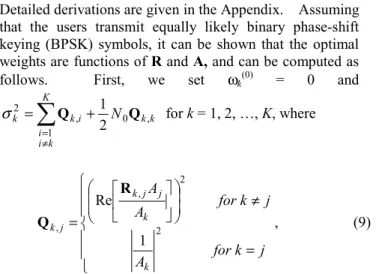
The average BER at 20 dB Eb/N0 are shown in Fig. 3
as functions of the number of users. Fig. 3 clearly shows that user ordering and the number of decision stages have significant impacts on performance, with the former being more important than the latter. Both perfect amplitude sorting (AS/g=30) and BER sorting (PS) with fewer stages significantly outperform the unsorted cases (AS/g=1) with more stages. Furthermore, the proposed algorithm with two stages outperforms the linear MMSE MUD even when g = 1. Finally, for both perfect amplitude sorting (AS/g=30) and BER sorting, NPWIC with S = 1 and S = 2 outperform conventional PIC and SIC.
The convergence curves of the different sorting algorithms are shown in Fig. 4. Here we set Eb/N0 = 30
dB, K=10, and S=1. The channel gains of the 10 users are 0.3597 + 0.3320j, 0.4682 - 0.3264j, -0.4669 - 0.8573j, -0.1698 - 1.1953j, -0.4726 - 0.6419j, 0.1459 + 0.8665j, -0.5757 + 1.6207j, -0.1801 - 0.2166j, 0.2046 - 0.4797j, and 0.7478 + 0.0943j. The UDO determined by perfect amplitude sorting (AS/g=10) and BER-sorting (PS) are shown in Table 1 along with UDO of the unsorted (AS/g=1) case. The average BER is plotted against user index in Fig. 4. It can be seen that perfect amplitude sorting converges to a lower BER than BER sorting. This means that although BER sorting outperforms amplitude sorting on average as shown in Fig. 3, for certain channels ampli-
Table 1. The decision orders under different methods Methods User permutated by decision order
AS/g=1 1 2 3 4 5 6 7 8 9 10 AS/g=10 7 4 3 6 5 10 2 9 1 8 PS 7 4 3 10 9 6 5 2 1 8
tude sorting performs better. Furthermore, as in Fig. 3, Fig. 4 also shows that the decision order has great impact on performance. 10 12 14 16 18 20 22 24 26 28 30 10-2 10-1 Eb/N 0 (dB) A v erage B E R AS/g=1, S=2, (unsort) AS/g=2, S=2, (quick-sort) AS/g=2, S=2, (pdf-sort) AS/g=4, S=2, (quick-sort) AS/g=4, S=2, (pdf-sort) AS/g=30, S=2, (sorted perfectly)
Fig. 2. Comparison of different user ordering in NPWIC MUD for
K=30. 0 5 10 15 20 25 30 10-2 10-1 number of user A v erage B E R SU-MF AS/g=1, S=1 PIC linear MMSE AS/g=1, S=2 SIC AS/g=30, S=1 PS, S=1 AS/g=30, S=2 PS, S=2
Fig. 3 Capacity figure of different WIC, SU-MF, PIC, SIC, linear MMSE MUDs under the condition of Eb/N0=20dB
1 2 3 4 5 6 7 8 9 10 10-6 10-5 10-4 10-3 10-2 10-1 user A v erage B E R AS/g=1, S=1 PS, S=1 AS/g=10, S=1
Fig. 4 Convergence rates and decision paths of different ordering methods under the condition of Eb/N0=30dB.
VI. CONCLUSION
A new multi-stage MUD referred to as NPWIC is proposed in this paper. Similar to PPIC, in the proposed MUD, decisions are weighted by reliability weighting factors when forming MAI estimates. However, unlike PPIC, an algorithm is also proposed to systematically jointly optimize the reliability weighting factors and user decision order. Simulation results show that the performance of proposed MUD is highly sensitive to the number of decision stages and decision orders. The proposed MUD significantly outperforms previously proposed methods and almost achieves the single user bound with just a few stages.
REFERENCES
[1] S. Moshavi, “Multi-user Detection for DS-CDMA Communications,”
IEEE Commum. Mag., pp. 124-136, Oct. 1996.
[2] Yue-heng Li, Ming Chen, Wang hai-feng, and Shi-xin Chen, “A Reduced Complexity Partial PIC detector,” Vehicular Technology Conference, 2001. VTC 2001 Fall. IEEE VTS 54th , Volume: 4 , 2001 [3] Yue-heng Li, Ming Chen, Wang hai-feng, and Shi-xin Chen, “Decision
Feedback Partial Parallel Interference Cancellation For DS-CDMA,”
MILCOM 2000. 21st Century Military Communications Conference Proceedings , Volume: 1 , 2000, Page(s): 579 -582 vol.2.
[4] Sergio Verdu, Multiuser Detection, Cambridge University Press, 1998.
[5] Thomas H. Cormen, Charles E. Leiserson, and Ronald L. Rivest,
Introduction to Algorithms, The MIT Press, Twentieth printing 1998.
[6] 3G TS 25.213 V4.1.0 “3rd Generation Partnership Project; Technical
Specification Group Radio Access Network; Spreading and modulation (FDD) (Release 4)”, 2001-06. http://www.3gpp.org.
[7] Divsalar, D.; Simon, M.K.; Raphaeli, D, “Improved parallel
interference cancellation for CDMA,” Communications, IEEE
Transactions on, Volume: 46 Issue: 2 , Feb. 1998, P.258 –268.
[8] Bong Youl Cho; Dohyung Choi; Sangkeun Lee; Youngmin Oh, “Performance of the improved PIC receiver for DS-CDMA over
Rayleigh fading channels,” Spread Spectrum Techniques and
Applications, 2000 IEEE Sixth International Symposium on, Volume: 1 , 2000, Page(s): 45 -49 vol.1.
[9] Sunghwan Kim; Jae Hong Lee, “Performance of iterative multiuser
detection with a partial PIC detector and serially concatenated codes,”
Vehicular Technology Conference, 2001. VTC 2001 Fall. IEEE VTS 54th , Volume: 1 , 2001 Page(s): 487 -491 vol.1.
APPENDIX:
A. Derivation of OptimalReliability Weighting Factors As mentioned earlier, the decision of the k-th user at the s-th stage can be expressed as
k s k s k m d dˆ()= () , (A.1) where mk(s) is a discrete random variable with at most M 2 possible values, where M is the cardinality of the signal constellation. Although the derivations to be presented can be extended to the general case, in the following we assume, for simplicity, that dk = 1 or –1 with equal likelihood for all k. In this case, we have
− = () ) ( ) ( -1 y probabilit with 1 y probabilit with 1 s k s k s k p p m , (A.2) where
(
ks k)
s k d d p() =Prob ˆ() ≠ . (A.3) Substituting (2) and (A.1) into (6), we have(
)
(
)
+ − + − + =∑
∑
+ = − − − = ) , ( ) , ( 1 (,) ) 1 ( ) , ( ) 1 ( ) , ( ) , ( ) , ( ), , ( ) , ( 1 1 (,) ) ( ) , ( ) ( ) , ( ) , ( ) , ( ), , ( ) , ( ) , ( ) ( ) , ( 1 1 1 1 Dec ˆ s k o s k o K k j o js s s j o s s j o s j o s j o s k o s k o k j o js s s j o s s j o s j o s j o s k o s k o s k o s s k o A n d m A A d m A A d d ω ω R R . (A.4) Since dk and mk(s) are real, we assume that ωo(j,s)(s) is also real.Dropping this assumption leads to the same result, but the derivation is more tedious. The real part of the quantity in the curly braces of (A.4) is given by
) , ( ) ( ) , ( ) , ( ) ( ) , ( ~ s k o s s k o s k o s s k o d MAI N d = + + , (A.5) where
(
)
(
)
∑
∑
+ = − − − = − + − = K k j s j o s s j o s s j o s k o s j o s j o s k o k j s j o s s j o s s j o s k o s j o s j o s k o s s k o d m A A d m A A MAI 1 ) , ( ) 1 ( ) , ( ) 1 ( ) , ( ) , ( ) , ( ) , ( ), , ( 1 1 ) , ( ) ( ) , ( ) ( ) , ( ) , ( ) , ( ) , ( ), , ( ) ( ) , ( 1 Re 1 Re ω ω R R (A.6) and = ) , ( ) , ( ) , ( Re s k o s k o s k o A n N . (A.7) If we assume that(
)
(
)
(
)
(
)
(
)
( ) ( ) ( 1) ( 1) ( , ) ( , ) ( , ) ( , ) ( , ) ( , ) ( ) ( ) ( ) ( ) ( , ) ( , ) ( , ) ( , ) ( , ) ( , ) ( 1) ( 1) ( , ) ( , ) ( , ) 1 1 0 1 1 0 1 1 s s s s o j s o l s o j s o j s o l s o l s s s s s o j s o l s o j s o j s o l s o l s s s o j s o j s o j s o E m d m d for j k l E m d m d for j l k E m d m ω ω ω ω ω − − − − − − = < < − − = < < −(
− ( 1) ( 1))
( , ) ( , ) ( , ) 0 < s s o l s l s− ωo l s− d for k j l = < (A.8) and mo(k,s)(s) is independent of do(k,s), then the variance ofMAIo(k,s)(s) + No(k,s) is given by
(
)
(
)
0 ( ,),( ,) 1 2 ) 1 ( ) , ( ) 1 ( ) , ( ) 1 ( ) , ( ) , ( ), , ( 1 1 2 ) ( ) , ( ) ( ) , ( ) ( ) , ( ) , ( ), , ( 2 ) ( ) , ( 2 1 ) ( ] [ 2 1 ) ( ] [ 2 1 s k o s k o K k j s s j o s s j o s s j o s j o s k o k j s s j o s s j o s s j o s j o s k o s s k o N m E m E Q Q Q + + − + + − ≡∑
∑
+ = − − − − = ω ω ω ω σ , (A.9)where Qo(k,s),o(j,s) is defined in (8). Furthermore, by the central limit theorem, when K is large MAIo(k,s)(s) and No(k,s) are
independent zero-mean Gaussian random variables. Therefore = () ) , ( ) ( ) , ( 1 s s k o s s k o Q p σ , (A.10) where Q(•) is the Gaussian tail function defined in (12). Thus, from (A.2) we have
− = () ) , ( ) ( ) , ( 1 2 1 ] [ s s k o s s k o Q m E σ . (A.11) It is desirable to minimize the average probability of error of the S-th stage given by
(
)
∑
= ≠ ≡ K k k S k av K probd d P 1 ) ( ˆ 1 , (A.12)(A.9) to (A.11) can be used recursively to express Pav in terms of all the decision orders and weightings, so in principle the jointly optimal decision orders and weightings that minimize Pav can be found. Unfortunately, this task is mathematically intractable. A more practical approach is to optimize the weightings on a stage-to-stage basis first. Specifically, for every s, ωo(j,s)(s), j = 1…K are chosen such
that po(k,s)(s) is minimized for all k. Since minimizing po(k,s)(s) is equivalent to minimizing σ o(k,s) (s), it can be seen from (A.9)
and (A.11) that the optimal weightings are given by
− = = () () ) ( [ ] 1 2 1 s j s j s j Em Q σ ω . (A.13) Using the optimal weighting in (A.13) implies that only the mean MAI is subtracted from each user’s signal, and intuitively should outperform the conventional PIC. Substituting (A.13) into (A.9), we have
(
)
(
)
0 ( ,), ( ,) 1 2 ) 1 ( ) , ( ) , ( ), , ( 1 1 2 ) ( ) , ( ) , ( ), , ( 2 ) ( ) , ( 2 1 ) ( 1 ) ( 1 s k o s k o K k j s s j o s j o s k o k j s s j o s j o s k o s s k o N Q Q Q + − + − =∑
∑
+ = − − = ω ω σ , (A.14)(A.13) and (A.14) can be used recursively from s = 1 to s = S to obtain the optimal weightings, with the initial values given by ωo(j,s)(0) = 0 for all j.
The computational complexity of evaluating (A.14) can be reduced by noting that
(
)(
)
(
)(
)
∑
∑
+ = − − − − − = − − − − + − − + − = K k j s s j o s s j o s s j o s s j o s j o s k o k j s s j o s s j o s s j o s s j o s j o s k o s s k o s s k o 1 ) 2 ( ) , ( ) 1 ( ) , ( ) 2 ( ) , ( ) 1 ( ) , ( ) , ( ), , ( 1 1 ) 1 ( ) , ( ) ( ) , ( ) 1 ( ) , ( ) ( ) , ( ) , ( ), , ( 2 ) 1 ( ) , ( 2 ) ( ) , ( ω ω ω ω ω ω ω ω σ σ Q Q . (A.15) Therefore, instead of directly computing (A.14), it is more efficient to update σo(k,s)(s) every time (A.13) is evaluated. In other words, when ω o(k,s) (s) is computed, σj(s)2 is immediately replaced by(
)(
( 1))
) , ( ) ( ) , ( ) 1 ( ) , ( ) ( ) , ( ) , ( , 2 ) ( − + − − s− s k o s s k o s s k o s s k o s k o j s j ω ω ω ω σ Q , (A.16) for all j≠o(k,s). The resulting algorithm is given in Section 4.B. User Ordering
As mentioned earlier, the UDO is optimized on a stage-to-stage basis. In this paper, two algorithms for user ordering are introduced: amplitude sorting and BER sorting. In amplitude sorting, K users are separated into g groups, Θ1,
Θ2,…., Θg, by sorting |Ak|2 such that for α < β < g, |Ai|2≥|Aj|2 for all i ∈ Θα and j ∈ Θβ. Assuming that the user indices in
the i-th group is given by
{
i i i i}
i ≡ θ,1,θ,2,L,θ,λ
Θ (A.17) where λi is the number of users in the i-th group, clearly we have λ1+….+λK=K. The decision order is given by
[
o(1,s),L,o(K,s)]
=[
θ1,1,L,θ1,λ1,LL,θg,1,L,θg,λg]
,(A.18) Note that when g=K, the decision order is determined by perfect amplitude sorting, i.e.,
2 ) , ( 2 ) , 2 ( 2 ) , 1 ( s o s o Ks o A A A ≥ ≥L≥ . (A.19) On the other hand, when g=1, the decision order is randomly chosen, i.e.,
[
o(1,s),L,o(K,s)] [
= 1,2,3,L,K]
. (A.20) In a flat-fading channel, amplitude sorting can be performed once the channel gains are estimated.In BER sorting, the decision order by finding the user with minimum BER as the next user to detect. Since finding the minimum BER is equivalent to finding the minimum σk(s)2, therefore every time (A.16) is evaluated,
the next user to detect can be determined by
{ } 2 ) ( ) , 1 ( ) , 1 ( min arg ) , ( ks s i o s o k s i o σ − ∉ = L , (A.21)