Optimal Energy-Efficient Routing for Wireless Sensor Networks
Chih-Wei Shiou, Frank Yeong-Sung Lin, Hsu-Chen Cheng, and
Wen
Department
of Information Management, National Taiwan University
yslin;
edu.
Abstract
The network for wireless sensor network plays an important role to survivability, Thus, we indicate the importance of routing protocol to network lifetime, and model the expected retransmission time as a convex function with respect to aggregate jlow on each sensor
node. Thus we formulate the optimal energy-eficient routing as a non-linear min-max programming problem with convex product form, which can be optimally solved by optimal routing framework. Based on the optimal routing framework, we propose Lagrangean-based algorithm and primal optimal algorithm. By the combination of these two algorithms, we can optimally and get the routing assignment to maximize the network life inthe sensor network.From experiments, we observe that when the optimal network lifetime increases
asthe number of sensor nodes increase. While the shortest path-based heuristic algorithm can only achieve about
48% network lifetime compared to our solution approach.
1. Introduction
In the wireless sensor network, the energy aware routing (EAR) protocol was presented to extend the network life time [4] TheEAR requires hardware support which is the capability of knowing the battery status, how many watts the node still remains. In this concept was enhanced by introducing “altruist”, the node having surplus energy to forward traffic, into wireless sensor networks. Through properly exchanging battery status between neighbors, the routing policy is energy efficient and the network life time extends significantly.
Since there are only a few OD (Original Destination) pairs needed to be recorded in each node’s routing table, we can compute several candidate routing paths for each OD pair. The benefit of multiple candidate routing paths was argued in We apply the features of optimal routing when selecting the candidate paths and scaling traffic flow between paths until the optimality conditions are satisfied.
Inthis paper, we choose table-driven routing policy and apply distance vector based algorithm, distributed Bellman-Ford (DBF) algorithm. To take the advantage of
the asynchronous convergence property of DBF we
build a routing protocol implemented with distributed fashion which is indispensable in practice for sensor networks. To apply optimal routing features on DBF, we have to define the link length as sophisticated parameters which are capable of affecting network life time as in and
Based the analysis of the expected retransmission time and the collision probability in wemodel the expected retransmission time as a convex of aggregate traffic load on the node then take it into the proposed routing algorithm. In the author proposed that min-max node lifetime objective function tends to find longer path resulting to decrease average node lifetime. Our algorithm contributes to keep balance between minimum node lifetime and average node lifetime in this stage.
The sensor deployment component is for topology determination Note that the sensor network topology is non-regular and usually randomly spread as We formulate the energy routing problem as a nonlinear optimization problem. Tofulfill the timing and the quality of the optimal decisions, the solution approach to the mathematical problem is Lagrangean relaxation method. In the further computational experiments, our proposed routing algorithm is expected to be efficient and effective to deal with each complexity problems.
The remainder of isorganized as follows. In Section2,we briefly describe the optimal energy routing problem and present the problem formulation. In Section 3, the solution approach is presented. In Section 4,
illustrate algorithms to solve the optimal mathematical problem and compare with other methods with experimental results in section5.Finally, we present our conclusionsin Section 6.
2. Problem description
In sensor networks, the interference is a significant effect on communication, which will affect bit-error rate and retransmission. To get an over-estimated retransmission model, consider the pure-aloha MAC formulation which can be taken as a performance lower-bound of thoseMAClayers in practice:
herehis the throughput of the transmitter node, defined as
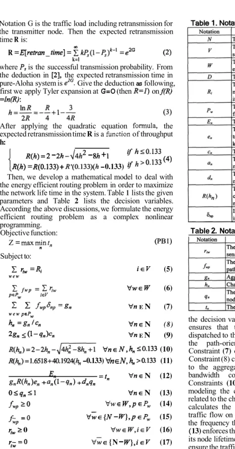
NotationG is the traffic load including retransmission for the transmitter node. Then the expected retransmission time R is:
2G
k=l
R= = =
where is the successful transmission probability. From the deduction in the expected retransmission time in pure-Aloha system is Give the deduction asfollowing, first we apply Tyler expansion at
G=O
(then onAfter applying the quadratic equation the expected retransmission time R is a of throughput
h:
-
-
+
= -0.133)
Then, we develop a mathematical model to deal with the energy efficient routing problem in order to maximize the network life time in the system. Table 1 lists the given parameters and Table 2 lists the decision variables. According the above discussions, we formulate the energy efficient routing problem as a complex nonlinear programming. Objective function: Subject to: Z= = w e w f w p = (5) (6) EN (7) w e w N (8) EN (9) (10) -0.133) (11) N (12) N (13) (14)
-
(15) 0 (16) {N-
(17) + +The objective function is to maximize the network lifetime of the given wireless sensor network configuration. The network lifetime is related to the routing policy and passive mode management, which are
Table2.Notation descriptionsfor decision variables
the decision variables in our formulation. Constraint (5)
ensures that the event-driven traffic can be fully dispatched to the corresponding sensors. Constraint (6) is the path-oriented routing requirement constraint. Constraint (7) calculates the aggregate flow on node n. Constraint (8) calculates the channel throughput according to the aggregate flow on node n. Constraint (9) is bandwidth constraint on wireless sensor nodes. Constraints (10) and (11) are both convex
modeling the expected number of retransmission time related to the channel throughput of node Constraint (12) calculates the node lifetime concerning the aggregate traffic flow on node n, the energy consumption rate and the frequency that node n is in passive mode. Constraint
(13)enforces the portion that node n is in passive mode of its node lifetime is between 0 and 1 . Constraints (14)-(17) ensure the traffic flow are positive or zero.
Because the node lifetime must be positive, the original objective function can be rewritten as following:
=min
+
-
+
Also, at the optimum, the passive mode must be fully utilizeto achieve the best energy-efficient. Constraint is active andq, Thus an equivalent formulation of Problem is:
Objective function:
Z=
Subject to:(5)
-
(17) except and (13). This re-formulation eliminatesand (13) as well as decision variables by merging them into the objective function and the problem becomes a single decision variable programming problem.
3.
Solution approach
The optimal routing problem (OEERP) in wireless sensor networks is a nonlinear programming problem with convex product form. We apply Lagrangean Relaxation (LR), which has been successfully adopted to solve many famous NP-complete problems to solve the optimal routing problem. By Lagrangean strong duality the tightest lower bound attained by Lagrangean dual problem is exactly the primal feasible objective function We also conduct a primal algorithm to get the optimal routing assignment resulting to maximize network lifetime.
We transform the maximization problem to minimization without loss of correctness.
Let
,
thenan equivalent formulation of Problem is: Objective function: Subject to:= mins s > o (5)
-
7) except 2), and (1 3). Vn N (20) Constraint (1 9) ensures the equality with original problem Constraint (20) defines the minimum node lifetime in the network. By using the LR the primal problem can be transformed into the following LR problem where Constraint (20) is relaxed. Foravector of non-negative Lagrangean the LR problem is given by optimizationproblem as:Objective function:
=
+ +
Subjectto:(5) (19) except (12), (1 3) and (1 8). In this formulation, a is the vector of which are Lagrangean multipliers and a, 0 . To solve this problem,
Subproblem(SUB2-2): related with decision variables Objective function:
+ Subject to: (11) and
i V
Vn N
vector is updated by = The step size is determined by , where the primal objective function value for a heuristic. It is an upper bound on
We describe the solution procedure of optimal routing as Fig. and the detailed description of each procedure is:
a. Computing First Derivative Length
By definition, the cost of Subproblem that the object is to minimize the sum of reciprocal of node lifetime weighted by Lagrangean multipliers, and the FDLis the first derivation with path flow. We get the first derivative length as following:
Given the valuation of first derivative length as mentioned above, at every iteration we compute each node’s lifetime according the current routing assignment, and recognize the bottleneck node in the network. Then update the first derivative length of all the paths. Finally we shift flow between paths basedon the first derivative length computed earlier. Repeat these steps until algorithm converge.
Our goal is to find the most economic path to shift positive flow iteration by iteration. By the lemmasof
optimal routing framework, the most economic and energy-efficient path must with the minimum sum of Node-FDL. Thus we directly apply Dijkstra shortest path algorithm to find the MFDL path for each OD-pair iteration by iteration, where the length computed for shortest path is the node-FDL.
We shift positive amount of flow form the maximum FDL path to the minimum one by applying Newton method on line search. Let be the step size that minimizes
+
(x’-
x)] over all between0 and1,that is,
b. Finding Path
c.Path Flow Adjustment
+
x)] =+
x)]The procedure above is a special case of the so-called Frank-Wolfe method for solving nonlinear programming problems with convex constraint sets.
Step Initialization.Set the iteration counterk to be Precalculate all the candidate pathsof each OD-pairs and any arbitrary one of feasible routing assignment set.
Step 2: Stopping.If is greater than a pre-specified counter then stop.
Computing.Update the aggregate flow on each node in the network accordingtothe currentrouting assignment. Step4 Updating.Compute node-FDL and path-FDL accordingto the
up-to-date aggregate flow.
Shiftiig Flow. Shift flow between paths according to path-FDL. Increase k by andgoto Step2.
Figure 1.An optimal energy-efficient routing algorithm
4.
routing algorithm
The primal optimal algorithm is similar with that we use to solve Lagrangean Subproblem However, the procedures including computing path FDL phase, finding path phase, and flow adjustment phase are different. This difference is resulted the min-max behavior and the differential property. We will give a detailed description of min-max Dijkstra algorithm as followings:
a. Finding Minimum Capacity CutPath
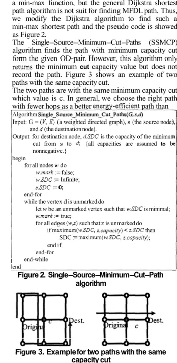
Because the objective function in our primal problem is a min-max function, but the general Dijkstra shortest path algorithm is not suit for finding MFDL path. Thus, we modify the Dijkstra algorithm to find such a min-max shortest path and the pseudo code is showed as Figure 2.
The Single-Source-Minimum-Cut-Paths (SSMCP) algorithm finds the path with minimum capacity cut form the given OD-pair. However, this algorithm only
the minimum cutcapacity value but does not record the path. Figure 3 shows an example of two paths with the same capacity cut.
Thetwo paths are with the same minimum capacity cut which value is c.In general, we choose the right path with fewer hops as a better path than
Algorithm
Input: G= (a weighted directed graph), s (the source node: Output: for destination node, is the capacity of the
cut from s to {all capacities are assumed to b nonnegative.}
for all nodes do
and (the destination node).
begin
:=false;
:=Infinite;
:=0;
end-for
while the vertex d is unmarked do
let be an unmarked vertex such that is minimal; true;
for all edges such that z is unmarked do
if then end if SDC:= end-for end-while lend Figure 2. Single-Source-Minimum-Cut-Path algorithm est.
3. Examplefortwo paths with the same capacity cut
the left. But the SSMCP algorithm may still possible return the left path. So based on the output of SSMCP algorithm,we apply modified Dijkstra algorithm to find the shortest and minimum cut path. Figure 4 shows the pseudo-code of Capacity- Constrained-Shortest-Path (CCSP) is for this purpose.
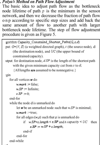
The basic idea to adjust path flow as the bottleneck node lifetime of path is the minimum in the sensor network, and then we decrease the fraction of path flow o n p according to specific step sizes and add back the same amount of flow to another path with larger bottleneck node lifetime. The step of flow adjustment procedure is given as Figure 5.
b. Method on Path Flow Adjustment
put: (a weighted directed graph), (the source node), d (the destination node), and (the upper bound of constrained capacity).
with the given minimum capacity cut from to {All lengths are assumed tobenonnegative.}
utput: for destination node, is the length of the shortest path
:gin
for all vertices wdo
:=false; Infinite;
:=0;
end-for
while the node d is unmarked do
letwbe an unmarked node such that is minimal; :=true;
for all edges such that is unmarked do
:= + if and then end-if end-for end-while ,
Step1: Initialization.Set the iteration counter k to be1.Compute the path bottleneck lifetime according to any given feasible routing assignment.
Stopping.If k is greater than a pre-specified counter limit then stop.
Finding.Find the paths with minimum and maximum bottleneck lifetime.
Selection.Select path with minimum bottleneck lifetime and denote its flow Shift the by a positive
.More precisely, we shift flow with amount of form the path with minimum bottleneck lifetime Step 2:
Step4:
k
5.
Experimental results
The experimentation variable is defined as the ratio between the edge lengths of grid area and the sensor's communication radius. The experimental result is given as Table 3. In wireless sensor networks, the communication radius is about 12.5 meters and 8 the area size is
100 meters. We adopt the energy consumption parameter of EYES-nodes in our study. For each sensor node, the parameters are as follows:
Wireless channel capacity is 10kbps.
Initial battery capacity of each sensor node is between 1300 and 1600 Watts.
Energy consumption rate on receiving (transmitting) is0.2Watts per byte.
Energy consumption rate to retain in active mode (passive mode) is 50 (10) Watts per second respectively.
In our computational experiments, we generate several system scenarios with different (1) average package length and (2) sensor node density. Then we apply the primal optimal algorithm introduced in Section 3 and Section4to compute the maximum network lifetime.
To experiment (1) average package length, we set up two cases with different parameters.In Case 1, the area size ratio 4. Here we set the number of nodes in Case 1 is 27, which is 1.5 times the minimum number of sensor nodes from Table3.And traffic demand is set as 5 which is 0.2 times the number of sensor nodes. In Case 2, the area size ratio. is 8, and we set up parameters according to the 'same logic as in Case 1. The experimental results are given in Table4.
To experiment (2) sensor node density, we set up two cases with different parameters. In Case3,the area size ratio is4.Here traffic demand is fix at 6 and average packet length is 200 bytes. The numbers of nodes are 1.5,
2.5, 3.5, and 4.5 times the minimum number of sensor nodes satisfying So they are 27,45, 63,
and 81 respectively. In Case4,the area size ratio- 8.
Those parameters in both Cases are list below, and the experimental results are given in Table 5.
In Table 4, we evaluate the effect of the expected retransmission time function which is consistent with our convex function to the aggregate flow on each sensor node Table 5 shows how the connectivity and the number of sensor node affect the network lifetime. It is clear that if the number of sensor nodes increases, it is with higher probability the network topology has higher connectivity. Thus the average network lifetime increase.
Figure 6 shows the network lifetime comparison between our primal optimal algorithm (PO) and Short-based algorithm (SP), which adopt the Dijkstra algorithm. Even though the path is the shortest path from the point of view with node lifetime and energy-efficiency, it is still fragile if any one bottleneck node exhaust it battery life. While our PO algorithm use multiple paths to route traffic between every OD-pairs, and the network
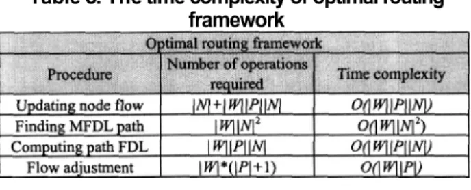
lifetime increase as the number of sensor nodes increases. We measure the primal optimal algorithm with time-complexity. The and denote the number
ofsensor nodes, the numberofOD-pairs, the numberof
candidate paths of each OD-pair, respectively. Table 7
shows the number of operations required and time complexity of optimal routing framework for one iteration. 100 300 500
6.
Conclusions
14925 665.9 4075 50.4 844 17.0In this paper, we address the importanceof routing protocol on energy Our proposed LR-based algorithm can efficiently get the near-optimal solution and the primal algorithm can optimally solve the problem but spending much more time. Both of them are variationsof
optimal routing framework, which is to optimally solve the multi-commodities routing problem. We appraise the marginal cost of candidate paths by in LR-based algorithm and by capacity cut in primal optimal algorithm respectively. Using the quantity we adjust flow between paths for each OD-pair until the two optimal conditions are satisfied. Then we eventually achieve the optimal routing which is energy-efficientweighted load-balancing.
27 45 63 :
...
...
...
..
I
23194 123 23901 418 28544 1035Table 6. The time complexity of optimal routing framework
7.
References
A., Wireless Sensor Network Designs, John Sons, Ltd. 2003.
Tanenbaum A. Networks, Fourth Edition, Prentice-Hall, 2002.
A. R. Shah, J. Rabaey and A. “Altruists in the Sensor Network”, International Workshop on Factory Comm. Systems (WFCS),
C. E., Ad Networking,Addison-Wesley, 2000.
C. K. To, “Maximum Battery Life Routing to Support Ubiquitous Mobile Computing in Wireless Ad Networks”, IEEE
Communications Magazine, 2001.
C. V. S. Ganeriwal and M.
“Optimizing Sensor Networks in the Energy-Latency-Density Design Space”, IEEE on Mobile 2002. Bersekas D. and R. Gallager, Networks,Prentice-Hall, 2nd edition, 1992,
E. andK. Bridges, “The Application of Remote Sensor Technology to Assist the Recovery of Rare and Endangered Species”, Special issue on Distributed Sensor Networks for
Journal of High Computing Applications, 2002.
GBianchi, Analysis of the IEEE 802.1 Distributed Coordination Function”, Select. Comm.,
...
...
Zussman andA. in AdI
...
....
...
I
Figure 6. Comparing network lifetime between PO and SP
Table3.Minimum number of sensor nodes to
Table4.Experimentalresultsforaverage packet
Table5.Experimentalresults for sensor node number
Network
Sensornodes
Case 3
I
Case4. . .
Disaster Recovery IEEE INFOCOM 2003. J. J. Garcia-Luna-Aceves, and T.
Practical Approach to Minimizing Delays in Routing,” IEEE 1999.
Held, and H. P. Crowder, “Validation of Optimization,” Math. Programming, 1974,pp.62-88.
L. Fisher, “The Relaxation Method for Solving Integer Programming Problems”, Science, 1981,
[ R. Gallager, “A Minimum Delay Routing Algorithm Using Distributed Computation”, IEEE Trans. Comm., 1977,
L. and A. Santhanam, “Optimal Routing, Link Scheduling and Power Control in Multi-hop Wireless Networks”, Proc. of IEEE INFOCOM 2003.
Kannan,S. S. S. andL.Ray, “Sensor-Centric Quality of Routing in Sensor Networks”, Proc. of IEEE INFOCOM 2003.
R. K., T. L. andJ. B. Network Flows: Theory,
and Hall, 1993.
C. Shah and J. M. Rabaey, “Energy Aware Routing for Low Energy Ad Sensor Networks”, Proc. of IEEE Wireless Comm. and networking Conference (WCNC), 2002.
Dam, and K. “An Adaptive Energy-Efficient MAC Protocol for Wireless Sensor Networks”, Proc. of The First ACM Conference on Embedded Networked SensorSystems, 2003.