可調式數位濾波器之設計

全文

(1)國立高雄大學電機工程學系碩士班碩士論文. 可調式數位濾波器之設計 Design of Variable Digital Filters. 研究生：張閔涵撰指導教授：徐忠枝博士. 中華民國 99 年 6 月.

(2)

(3) 可調式數位濾波器之設計. 指導教授：徐忠枝博士國立高雄大學電機工程學系. 學生：張閔涵國立高雄大學電機工程學系碩士班. 摘要本篇論文主要在研究可調式數位濾波器之設計。近十幾年來在通訊、訊號處理、影像處理領域，可調式數位濾波器(Variable Digital Filters)都受到相當的重視與廣泛的應用。因為具有可調的參數，需要不同的響應或延遲可以立即地調控，不用再重新設計。依照可調的情況不同，我們將分為可調式分數延遲濾波器(Variable Fractional-Delay filters)與可調式分數階微積分器 (Variable Fractional-Order differintegrators)二大類進行探討。我們提出了權重式最小平方差逼近法(Weighted Least-Squares Approach)來設計有限脈衝響應(Finite Impulse Response)、無限脈衝響應(Infinite Impulse Response)、全通(Allpass)濾波器。此設計不但可以達到我們預期的成果，在一定範圍內更呈現了極小的誤差。接著在可調式分數階微積分器方面，分別設計了 FIR 與 IIR 的微積分器(differintegrators)。只要調整適當的參數，即可作為微分器、積分器，甚至同時具有微分與積分的功能。更重要的是，Farrow 架構(Farrow structure)已經可以成功地應用來實現上述可調式數位濾波器系統。. 關鍵字：可調式分數延遲濾波器、可調式分數階微積分器、FIR 微積分器、IIR 微積分器、權重式最小平方差逼近法、Farrow 架構。. i.

(4) Design of Variable Digital Filters. Advisor：Dr. Jong-Jy Shyu Department of Electrical Engineering National University of Kaohsiung. Student：Min-Han Chang Department of Electrical Engineering National University of Kaohsiung. ABSTRACT In this thesis, the major research is the design of variable digital filters. During the past decade, variable digital filters have received considerable attention because they were widely used in communication systems, signal processing and image processing. Different responses or delays can be immediately obtained by tuning the variable parameters without the need to design a new one. The designs of variable digital filters are often classified into two categories according to various adjustable situations, which are the variable fractional-delay (VFD) digital filters and the variable fractional-order (VFO) differintegrators. First, Weighted Least-Squares Approach (WLS) is proposed to design the FIR, IIR and Allpass variable fractional-delay filters. This method not only can achieve the desired performance but also minimize the errors in the design range. Then, the topic is focused on the variable fractional-order (VFO) differintegrators. Both FIR differintegrator and IIR differintegrator are designed. They can deal with derivatives or integrals or even compute derivatives and integrals in the same filter by simply adjusting proper parameters. Importantly, the Farrow structure has successfully been applied to implement the variable digital filter systems stated above.. Keywords:. Variable fractional-delay filter, variable fractional-order differintegrator, FIR differintegrator, IIR differintegrator, weighted least-squares approach, Farrow structure.. ii.

(5) 致謝經過了這些日子的努力，終於完成了這篇論文。當然，最要感謝的是我的指導教授徐忠枝老師。您是我生命中的貴人，不論在研究上或生活上，您努力認真、謙遜負責的態度，就是最好的身教。對於您的一路照顧，我的心中更是充滿說不盡的感激。接下來我要感謝我最好的夥伴振洋，一直對你的沉穩細心感到佩服，你是我另一個學習的榜樣。還要感謝曾經一起修課的高科大的學長們，尤其是斯弘學長，他無私的指導與關心，讓我無比地動容。再來要感謝諸位口試委員，因為有了你們的指點與建議，才能使這篇論文更為充實與完備。接著，我要感謝目前已在台大博士班的韻達，他總是熱心地幫了我許多忙。實驗室幽默的家墀學弟、聰明的亦閎、酷酷的旺業、見聞廣博的耀興，以及兩位可愛亮眼的美女學妹皓婷和嶼芝，能夠認識你們真好。對於學校的各方面事務，則是要感謝系辦薏婷和佳恬的辛苦幫忙。其實這一路走來，要感謝的人真的太多太多，但限於篇幅實在無法一一列名，僅在此一併表示我最誠摯的敬意。最後，我的家人們，爸爸媽媽、大哥、二哥是我背後最溫暖的支持。因為有你們不斷的栽培與鼓勵、無怨無悔的付出，讓我可以心無旁務地完成碩士學業。而今，我將邁向人生的下一個階段，我要告訴大家這段時間我真的成長了很多。僅將此論文獻與上述我所感激的每一位，是你們造就了今日的我，你們的恩情，閔涵永難忘懷。張閔涵. iii. 於高雄大學 2010 年 6 月.

(6) Contents Abstract (In Chinese) ………………………………………………………………………………..i Abstract (In English) ………………………………………………………………………………..ii Acknowledgement (In Chinese) ……………………………………………………………………iii Contents ……………………………………………………………………………………………..iv List of Figures .……………………………………………………………………………………...vi. Chapter 1.. Introduction…………………………………………………………………………. 1. Chapter 2.. Design of Variable Fractional-Delay FIR Filters ………………………………….. 2. 2.1. Introduction ……………………………………………………………………………….2. 2.2. Problem Formulation …………………………………………………………………….2. 2.3 Using Weighted Least-Squares Approach to design VFD FIR filters …………………5 2.4. Numerical Example ………………………………………………………………………7. 2.5. Conclusions ………………………………………………………………………………..9. Chapter 3.. Design of Variable Fractional-Delay IIR Filters ………………………………… 10. 3.1. Introduction ……………………………………………………………………………..10. 3.2. Problem Formulation …………………………………………………………………..10. 3.3 Using Weighted Least-Squares Approach to design VFD IIR filters ………………...12 3.4. Numerical Example ……………………………………………………………………..15. 3.5. Conclusions ………………………………………………………………………………18. Chapter 4.. Design of Variable Fractional-Delay Allpass Filters …………………………….. 19. 4.1. Introduction ……………………………………………………………………………..19. 4.2. Problem Formulation …………………………………………………………………..19. 4.3. Using Weighted Least-Squares Approach to design VFD Allpass filters ……………22. 4.4. Numerical Example ……………………………………………………………………..24 iv.

(7) 4.5. Conclusions ………………………………………………………………………………26. Chapter 5.. Design of Variable Fractional-Order FIR Differintegrators ……………………. 27. 5.1. Introduction ……………………………………………………………………………...27. 5.2. Problem Formulation …………………………………………………………………...27. 5.3. VFO FIR differintegrator, pure differentiator and pure integrator examples ……...33. 5.4. Conclusions ………………………………………………………………………………37. Chapter 6. Design of Variable Fractional-Order IIR Differintegrators ……………………. 38 6.1 Introduction ……………………………………………………………………………….38 6.2 Problem Formulation ……………………………………………………………………..38 6.3 VFO IIR differintegrator, pure differentiator and pure integrator examples ………...45 6.4 Conclusions ………………………………………………………………………………..49 Chapter 7.. Conclusions and Future works ……………………………………………………..50. Reference …………………………………………………………………………………………51. v.

(8) List of Figures Fig. 2-1. Farrow structure of a VFD FIR digital filter. Fig. 2-2 Design of a VFD FIR digital filter with N = 60 , M = 9 , and ω p = 0.9π . (a) Magnitude response (b) Variable fractional-delay response (c) Absolute error of variable frequency response. Fig. 3-1. Farrow structure of a VFD IIR digital filter with N a = 3 , N b = 4 , M = 3. Fig. 3-2. Design of a N a = 14 , N b = 55 , M = 5 , ω p = 0.9π , and I = 27 VFD IIR filter. (a) Magnitude response (b) Absolute error of variable frequency response (c) Group-delay response (d) Absolute error of variable group-delay response.. Fig. 3-3. Design of a N a = N b = I = 35 , M = 5 , ω p = 0.9π , VFD IIR filter. (a) Magnitude response (b)Absolute error of variable frequency response (c) Group-delay response (d) Absolute error of variable group-delay response.. Fig. 4-1. Farrow structure of an allpass VFD digital filter ( N = 5 , M = 4 ). Fig. 4-2 Design of an allpass VFD filter with N = 30 , M = 5 , ω p = 0.9π , p1 = −0.5 (a). Variable group-delay response (b) Absolute delay errors Fig. 5-1 FIR-typed Farrow structure Fig. 5-2 Design of a VFO differintegrator with N = 40 , M = 5 , ω s = 0.05π , ω p = 0.95π , ps = −0.5 , and p f = 0.5 (a) Variable magnitude response (b) Absolute error of variable. frequency response. Fig. 5-3 Design of a VFO differentiator with N = 30 , M = 6 , ωs = 0 , ω f = 0.9π , ps = 1 , and p f = 2 (a) Variable magnitude res ponse (b ) Abso lu te err or of va riable f r equency response.. vi.

(9) Fig. 5-4 Design of a VFO integrator with N = 60 , M = 6 , ωs = 0.05π , ω p = 0.9π , ps = −1.5 , and p f = −0.5 (a) Variable magnitude response (b) Absolute error of variable frequency response. Fig. 6-1 IIR-typed Farrow structure Fig. 6-2 Design of a N a = 11 , N b = 29 , M = 5 , ωs = 0.05π , ω p = 0.95π , ps = −0.5 , p f = 0.5 ,. α = 1.7782 7294 × 10 −5 and I = 19 VFO IIR differintegrator (a) Magnitude response (b) Absolute error of variable frequency response. Fig. 6-3 Design of a N a = 7 , N b = 2 3 , M = 3 , ω s = 0 , ω f = 0.9π , p s = 1 , p f = 2 ,. α = 1.77827294 ×10−4 and I = 14 VFO IIR differentiator (a) Magnitude respons e (b) Absolute error of variable frequency response. Fig. 6-4 Design of a N a = 15 , N b = 45 , M = 4 , ωs = 0.05π , ω f = 0.9π , ps = −1.5 , p f = −0.5 ,. α = 5.62341325 ×10−2 and I = 28 VFO IIR integrator (a) Magnitude response (b) Absolute error of variable frequency response.. vii.

(10)

(11) Chapter 1 Introduction. The variable digital filter design has become an important topic in recent years, which owned the self-adjustable ability online. Hence, the variable digital filters are useful for various applications, such as the design of comb filter, tunable modulator, sample-rate converter, discrete time signal interpolation and time delay estimation [1]-[4], etc. Generally speaking, the Farrow structure [5] can be applied to implement the variable digital filter systems. In this thesis, two types of variable digital filters are discussed, which are the variable fractional-delay (VFD) digital filters and the variable fractional-order (VFO) differintegrators, respectively. First, the VFD FIR filter is proposed for design. However, the VFD IIR, VFD Allpass filter designs must handle the stability problem. The constrained function would be incorporated into the objective error function to overcome this principal issue. Then, the differintegrators, including the pure differentiators and the pure integrators can be designed by the VFO FIR filters or the VFO IIR filters [6]-[13]. Similarly, it is significant important to ensure that the VFO IIR filters are stable. In particular, the related vectors or matrices in these designs can be derived as the closed-forms to simplify the calculation complexity. Several examples are presented to illustrate the desired results, which include the magnitude response, the group-delay response and the absolute error of variable frequency response, etc. Many techniques and methods are used to design these filters in this thesis, containing the symmetric/antisymmetric relationships, Weighted Least-Squares Approach (WLS), Binomial Series Expansion, Taylor Series Expansion, and quadratic methods [14]-[16], etc. This thesis is organized as follows: Chapter 1 is introduction. Chapters 2 to Chapter 4 concentrates on the VFD filter designs. Chapters 5 and 6 present the designs of the VFO diffintegrators. Finally, the conclusions and future works are given in the last chapter.. 1.

(12) Chapter 2. Design of Variable Fractional-Delay FIR Filters. 2.1 Introduction. The Variable Fractional-Delay (VFD) digital filter is a branch of variable digital filters. The online tunable property can be used in many aspects. As a result, many methods have been developed to design the VFD FIR filter such as Farrow structure, Lagrange-type method [17], and coefficient symmetric method [18]-[20], etc. Recently, Weighted Least-Squares Approach (WLS) has been successfully applied to the VFD FIR filter design. In this chapter, the problem formulation of the VFD FIR filter is presented in section 2.2. In section 2.3, a method is proposed to design the VFD FIR filter, which is Weighted Least-Squares Approach. Then, a design example is shown to demonstrate the effectiveness of this method in section 2.4. Finally, the conclusions of designing the VFD FIR filter are discussed in section 2.5.. 2.2 Problem Formulation. In this section, the problem formulation would be derived in detail. For designing a VFD FIR filter, the desired response is given by. 2.

(13) D (ω, p ) = e. −j. −j. N ω 2. ⋅ e− jω p. N ω 2. ⎡⎣cos (ω p ) − j sin (ω p ) ⎤⎦ −ω p ≤ ω ≤ ω p , −0.5 ≤ p ≤ 0.5 =e. (2.1). where N means the order and p means the variable fractional group-delay. The transfer function. N. H ( z, p ) = ∑ hn ( p ) z − n. (2.2). n =0. is used to approximate the desired response in (2.1). The coefficients hn ( p ) are expressed as the polynomials of parameter p. M. hn ( p ) = ∑ h ( n, m) pm. (2.3). m= 0. thus (2.3) becomes. N. M. H ( z , p ) = ∑ ∑ h ( n, m ) p m z − n n=0 m=0. M ⎛ N ⎞ = ∑ ⎜ ∑ h ( n, m ) z − n ⎟ p m m =0 ⎝ n =0 ⎠ M. = ∑ Gm ( z ) p m m =0. According to (2.4), it can be implemented by the Farrow structure as shown in Fig. 2-1.. Fig. 2-1 Farrow structure of a VFD FIR digital filter 3. (2.4).

(14) By the symmetric/antisymmetric properties of (2.1) with respect to p , (2.4) would be separated into odd part and even part as follows: Mc ⎛ N ⎞ H ( z , p ) = ∑ ⎜ ∑ h ( n, 2 m ) z − n ⎟ p 2 m m =0 ⎝ n=0 ⎠ Ms ⎛ N ⎞ + ∑ ⎜ ∑ h ( n, 2m − 1) z − n ⎟ p 2 m −1 m =1 ⎝ n = 0 ⎠. (2.5). where M ⎧ ⎪⎪ M c = M s = 2 , ⎨ ⎪M + 1 = M = M + 1 , s ⎪⎩ c 2. for even M (2.6) for odd M. In this topic, only even N is considered, and odd N can be developed similarly. Moreover, by the frequency characteristics of (2.1), the frequency response of the VFD FIR filter design can be derived as H (e , p ) = e jω. −j. N ω 2. ⎡ Mc N /2 2m ⎢ ∑ ∑ a ( n, m ) p cos ( nω ) ⎣ m=0 n=0 Ms N /2 ⎤ + j ∑ ∑ b ( n, m ) p 2 m −1 sin ( nω ) ⎥ m =1 n =1 ⎦. ( 2.7). where. a ( n, m ) ⎧ ⎛N ⎞ ⎪ h ⎜ 2 , 2m ⎟ ⎪ ⎝ ⎠ =⎨ ⎪ 2 h ⎛ N − n, 2 m ⎞ = 2 h ⎛ N + n, 2 m ⎞ ⎟ ⎜ ⎟ ⎪⎩ ⎜⎝ 2 ⎠ ⎝2 ⎠. n = 0, 0 ≤ m ≤ M c N 1≤ n ≤ , 0 ≤ m ≤ Mc 2. (2.8a ). b ( n, m ) ⎛N ⎞ ⎛N ⎞ = 2 h ⎜ − n, 2 m − 1 ⎟ = −2 h ⎜ + n , 2 m − 1 ⎟ ⎝2 ⎠ ⎝2 ⎠ N 1≤ n ≤ , 1≤ m ≤ Ms 2. In addition, substituting p = 0 into (2.1) and (2.7),. 4. (2.8b).

(15) D (ω , 0 ) = e. −j. N ω 2. (2.9a ). and. H ( e jω , 0 ) = e. −j. N N /2 ω 2. ∑ a ( n, 0 ) cos ( nω ). (2.9b). n=0. which result in. a ( n, 0 ) = δ ( n ). (2.10). So, (2.7) can be rewritten by (2.8a) and (2.8b). H ( e jω , p ) = e. −j. N ω 2. ⎡ M c N /2 2m ⎢1 + ∑∑ a ( n, m ) p cos ( nω ) ⎣ m =1 n =0 M s N /2 ⎤ + j ∑∑ b ( n, m ) p 2 m −1 sin ( nω ) ⎥ m =1 n =1 ⎦. (2.11). 2.3 Using Weighted Least-Squares Approach to design VFD FIR filters. Assume A is a. ( N / 2 + 1) × M c. matrix and B is a. ( N / 2) × M s. matrix, which are defined by. A = ⎣⎡ a ( n, m ) ⎦⎤. (2.12a). B = ⎡⎣b ( n, m ) ⎤⎦. (2.12b). and. The objective error function of the VFD FIR filter is. 5.

(16) Kω K p. (. e ( A, B ) = ∑∑W (ωi ) D (ωi , pl ) − H e jωi , pl i =0 l =0. = e ( A) + e (B) ,. ωi =. iω p Kω. , pl =. ). 2. 0.5l Kp. (2.13). where W (ω ) is a weighting function, and. M c N /2 ⎡ ⎤ e ( A ) = ∑∑ W (ωi ) × ⎢cos (ωi pl ) − 1 − ∑∑ a ( n, m ) pl 2 m cos ( nωi ) ⎥ i =0 l =0 m =1 n = 0 ⎣ ⎦ Kw K p. M s N /2 ⎡ ⎤ e ( B ) = ∑∑ W (ωi ) × ⎢ − sin (ωi pl ) − ∑∑ b ( n, m ) pl 2 m −1 sin ( nωi ) ⎥ i =0 l =0 m =1 n =1 ⎣ ⎦ Kw K p. Based on a. ( Kω + 1) × ( K p + 1). 2. (2.14a). 2. (2.14b). grid, Kω = 20 N and K p = 200 are used. So, (2.14a) and (2.14b). can be expressed in matrix forms as below: T e ( A ) = tr ⎡⎢( DA − CAPAT ) ( D A − CAPAT ) ⎤⎥ ⎣ ⎦ T T = tr ⎡⎢ DAT DA − DAT CAPAT − ( CAPAT ) DA + ( CAPAT ) ( CAPAT ) ⎤⎥ ⎣ ⎦. (2.15a ). and T e ( B ) = tr ⎡⎢( DB − SBPBT ) ( DB − SBPBT ) ⎤⎥ ⎣ ⎦ T T = tr ⎡⎢ DBT DB − DBT SBPBT − ( SBPBT ) DB + ( SBPBT ) ( SBPBT ) ⎤⎥ ⎣ ⎦. where tr (.) denotes a trace operator, and the superscript. T. (2.15b). denotes a transpose operator,. ⎡ 12 DA = ⎢W (ωi ) ( cos (ωi pl ) − 1) ⎣. ⎤ 0 ≤ i ≤ Kω , 0 ≤ l ≤ K p ⎥ ⎦. (2.16a ). 1 ⎡ DB = ⎢ −W 2 (ωi ) sin (ωi pl ) ⎣. ⎤ 0 ≤ i ≤ Kω , 0 ≤ l ≤ K p ⎥ ⎦. (2.16b). 6.

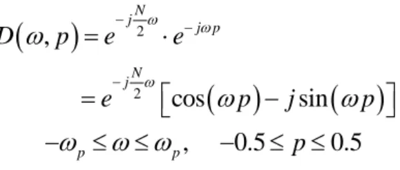
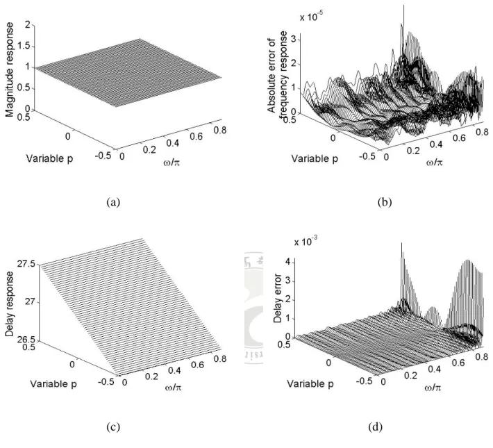
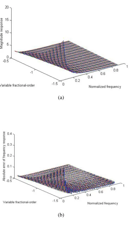
(17) ⎡ 12 C = ⎢W (ωi ) cos ( nωi ) ⎣. 0 ≤ i ≤ Kω , 0 ≤ n ≤. N⎤ ⎥ 2⎦. (2.16c). ⎡ 1 S = ⎢W 2 (ωi ) sin ( nωi ) ⎣. 0 ≤ i ≤ Kω ,1 ≤ n ≤. N⎤ ⎥ 2⎦. (2.16d ). PA = ⎣⎡ pl 2 m ,. 0 ≤ l ≤ K p , 1 ≤ m ≤ M c ⎤⎦. (2.16e). PB = ⎣⎡ pl 2 m −1 ,. 0 ≤ l ≤ K p , 1 ≤ m ≤ M s ⎦⎤. (2.16 f ). and. In order to solve A , e ( A, B ) is partial differentiated with respect to A and the result is set to zero, which can yield. A = ( CT C ) CT DA PA ( PAT PA ) −1. −1. (2.17). Similarly, B can be obtained as. B = ( ST S ) ST DB PB ( PBT PB ) −1. −1. (2.18). Finally, the absolute error of variable frequency response is defined by. E (ω , p ) = D (ω , p ) − H ( e jω , p ). 2.4. (2.19). Numerical Example. An example is presented to illustrate the effectiveness of the WLS technique in this section. Consider the design of a VFD FIR filter with N = 60 , M = 9 , ω p = 0.9π , W (ω ) = 1 , p ∈ [ 0, 0.5]. 7.

(18) in the example. Figs. 2-2(a) and (b) show the magnitude response and group-delay response. Furthermore, the absolute error of variable frequency response is presented in Fig. 2-2(c). Notice that, the frequency ω and the variable p are uniformly sampled at step sizes ω p / ( 20 N ) and 0.5/200, respectively.. (a). (b). (c). Fig. 2-2 Design of a VFD FIR dig ital fi lter with N = 60 , M = 9 ,and ω p = 0.9π . (a) Magnitude response (b) Variable fractional-delay response (c) Absolute error of variable frequency response.. 8.

(19) 2.5 Conclusions. In this chapter, WLS method was successfully applied to design the VFD FIR digital filter. By using the coefficient symmetric/antisymmetric technique, the number of filter coefficients which is needed for the design was reduced by about 50％. An example was presented to demonstrate the effectiveness in section 2.4. Besides, it was found that the weighting function depends only on the frequency ω , not on the tunable parameter p . So, this technique is a significant approach for designing the VFD FIR filter.. 9.

(20) Chapter 3. Design of Variable Fractional-Delay IIR Filters. 3.1 Introduction. After the discussion of the VFD FIR filter design in the previous chapter, this chapter introduces the design of VFD IIR filter. However, the VFD IIR filter is much more difficult to design since the stability problem must be handled [21]-[22]. Similarly, Weighted Least-Squares Approach (WLS) is used. The objective error function is formulated such that the stability constraint can be incorporated. This chapter is organized as follows: in section 3.2, the problem is formulated and the Farrow structure of the VFD IIR filter is proposed. Then, the stable condition is considered in the objective error function in section 3.3. Two examples are designed to demonstrate the effectiveness, which are presented in section 3.4. Finally, section 3.5 summaries the conclusions.. 3.2 Problem Formulation. For designing the VFD filters, the desired response is given by H d (ω , p ) = e − j ( I + p )ω , ω ∈ ⎡⎣0, ω p ⎤⎦. (3.1). where I is a prescribed integer group-delay and p is a adjustable parameter between -0.5 and 0.5. The transfer function of the variable IIR digital filter is characterized as 10.

(21) B ( z, p ) ∑ n=b0 bn ( p ) z − n H ( z, p ) = = A ( z , p ) 1 + ∑ N a an ( p ) z − n N. (3.2). n =1. which is chosen to approximate (3.1). where the filter coefficients an ( p ) and bn ( p ) are expressed as the polynomials of p an ( p ) = ∑ m =0 a ( n, m ) p m ,. 1 ≤ n ≤ Na. (3.3a ). bn ( p ) = ∑ m =0 b ( n, m ) p m ,. 0 ≤ n ≤ Nb. (3.3b). M. M. Substituting (3.3a) and (3.3b) into (3.2) can yield. ∑ ( ∑ b ( n, m ) z ) p H ( z, p ) = 1 + ∑ ( ∑ a ( n, m ) z ) p −n. M. Nb. m =0. n=0. M. Na. m=0. n =1. −n. m. m. which can be implemented by the Farrow structure as shown in Fig. 3-1.. Fig. 3-1 Farrow structure of a VFD IIR digital filter with N a = 3 , N b = 4 , M = 3 11. (3.4).

(22) 3.3 Using Weighted Least-Squares Approach to design VFD IIR filters. In this section, the WLS Approach would be introduced to solve the previous problem. The frequency response of the desired VFD IIR filter can be represented by b ( n, m ) p e ω b c ( ω , p ) − jb s ( ω , p ) ∑ ∑ = H (e , p) = 1 + ∑ ∑ a ( n, m ) p e ω 1 + a c (ω , p ) − ja s (ω , p ) jω. M. Nb. m=0 M. n =0 Na. m =0. where the superscript. m − jn. m − jn. n =1. T. T. T. b T. b T. a. (3.5). a. denotes a transpose operator,. a = ⎡⎣ a (1, 0 ) , ⋅⋅⋅, a ( N a , 0 ) , ⋅⋅⋅, a (1, M ) , ⋅⋅⋅, a ( N a , M ) ⎤⎦. T. (3.6a). c a (ω , p ) = ⎡⎣cos (ω ) , ⋅⋅⋅, cos ( N aω ) , ⋅⋅⋅, p M cos (ω ) , ⋅⋅⋅, p M cos ( N aω ) ⎤⎦ s a (ω , p ) = ⎡⎣sin (ω ) , ⋅⋅⋅,sin ( N aω ) , ⋅⋅⋅, p M sin (ω ) , ⋅⋅⋅, p M sin ( N aω ) ⎤⎦. T. T. (3.6b). (3.6c). and. b = ⎡⎣b ( 0, 0 ) , ⋅⋅⋅, b ( N b , 0 ) , ⋅⋅⋅, b ( 0, M ) , ⋅⋅⋅, b ( N b , M ) ⎤⎦. T. cb (ω , p ) = ⎡⎣1, ⋅⋅⋅, cos ( N bω ) , ⋅⋅⋅, p M , ⋅⋅⋅, p M cos ( N bω ) ⎤⎦ sb (ω , p ) = ⎡⎣ 0, ⋅⋅⋅,sin ( N bω ) , ⋅⋅⋅, 0, ⋅⋅⋅, p M sin ( N bω ) ⎤⎦. Thus, the approximation error function can be gotten as 12. T. (3.6d ). T. (3.6e). (3.6 f ).

(23) ea ( a, b) =∫. 0.5. =∫. 0.5. ∫. ωp. ∫. ωp. −0.5 0. −0.5 0. W (ω ) Hd (ω, p ) A( e jω , p ) − B ( e jω , p ) dωdp 2. W (ω ) ⎣⎡cos ( ( I + p ) ω ) − j sin ( ( I + p ) ω )⎦⎤ ⋅ ⎣⎡1 + aT ca (ω, p ) − jaT sa (ω, p ) ⎦⎤ − ⎡⎣bT cb (ω, p ) − jbT sb (ω, p ) ⎤⎦ dωdp 2. =∫. 0.5. ∫. ωp. −0.5 0. {. W (ω ) cos ( ( I + p ) ω ) + cos ( ( I + p ) ω ) aT ca (ω, p ) − sin ( ( I + p ) ω ) aT sa (ω, p ) − bT cb (ω, p ). + − sin ( ( I + p ) ω ) − sin ( ( I + p ) ω ) aT ca (ω, p ) − cos ( ( I + p ) ω ) aT sa (ω, p ) + bT sb (ω, p ). 2. 2. } dωdp (3.7). which can be rewritten as. ea ( x ) = ∫. ∫. ωp. 0.5. ∫. 0.5. −0.5 0. =∫. {. W (ω ) cos ( ( I + p ) ω ) + xT c (ω , p ) + sin ( ( I + p ) ω ) + xT s (ω , p ). ωp. −0.5 0. 2. {. 2. } dωdp. W (ω ) 1 + xT ⎡⎣ 2cos ( ( I + p ) ω ) c (ω , p ) + 2sin ( ( I + p ) ω ) s (ω , p ) ⎤⎦. }. + xT ⎡⎣c (ω , p ) cT (ω , p ) + s (ω , p ) sT (ω , p ) ⎤⎦ x dω dp (3.8) where W (ω ) means a weighting function, ⎡a ⎤ x=⎢ ⎥ ⎣b ⎦. (3.9a ). ⎡cos ( ( I + p ) ω ) c a (ω , p ) − sin ( ( I + p ) ω ) s a (ω , p ) ⎤ c (ω , p ) = ⎢ ⎥ −c b ( ω , p ) ⎢⎣ ⎥⎦. (3.9b). ⎡sin ( ( I + p ) ω ) c a (ω , p ) + cos ( ( I + p ) ω ) s a (ω , p ) ⎤ s (ω , p ) = ⎢ ⎥ −sb (ω , p ) ⎢⎣ ⎥⎦. (3.9c). So, (3.8) can be given in a quadratic form as ea ( x ) = s + xT r + xT Qx. (3.10). in which,. 13.

(24) s=∫. 0.5. ∫. ωp. −0.5 0. r=∫. 0.5. ∫. ωp. −0.5 0. Q=∫. 0.5. ∫. W (ω )d ω dp. (3.11a ). W (ω ) ⎡⎣ 2 cos ( ( I + p ) ω ) c (ω , p ) + 2sin ( ( I + p ) ω ) s (ω , p ) ⎤⎦ d ω dp. ωp. −0.5 0. W (ω ) ⎡⎣c (ω , p ) cT (ω , p ) + s (ω , p ) sT (ω , p ) ⎤⎦ dω dp. (3.11b). (3.11c). Concerning the stability of the VFD IIR filter, it has been shown in [22] that. Na. Na. n =1. n =1. 1 + ∑ an ( p ) cos ( nω ) ≥ 1 − 2∑ an 2 ( p ). when. ∑. ∑. (3.12). a ( p) is less than 0.5, the desired filter is stable for the specified p . Hence, the value of. Na 2 n=1 n. a ( p) must be small enough to satisfy the stable condition. The constrained function is defined. Na 2 n=1 n. by ⎛ Na 2 ⎞ an ( p ) ⎟dp ⎜ ∑ −0.5 ⎝ n =1 ⎠. ec ( a ) = ∫. 0.5. (3.13). where. 2. ⎛ M m⎞ T T = a p ( ) ∑ ∑ n ⎜ ∑ a ( n, m ) p ⎟ = x PP x n =1 n =1 ⎝ m = 0 ⎠ Na. Na. 2. (3.14). and. P = ⎡⎣ I Na , pI N a , ⋅⋅⋅, p M I N a , 0 ⎤⎦. T. (3.15). In (3.15), I Na means an Na × Na identity matrix and 0 represents a Na ×( Nb +1)( M +1) zero matrix. By substituting (3.13) and (3.14) into (3.15), the constrained function would be achieved as. 14.

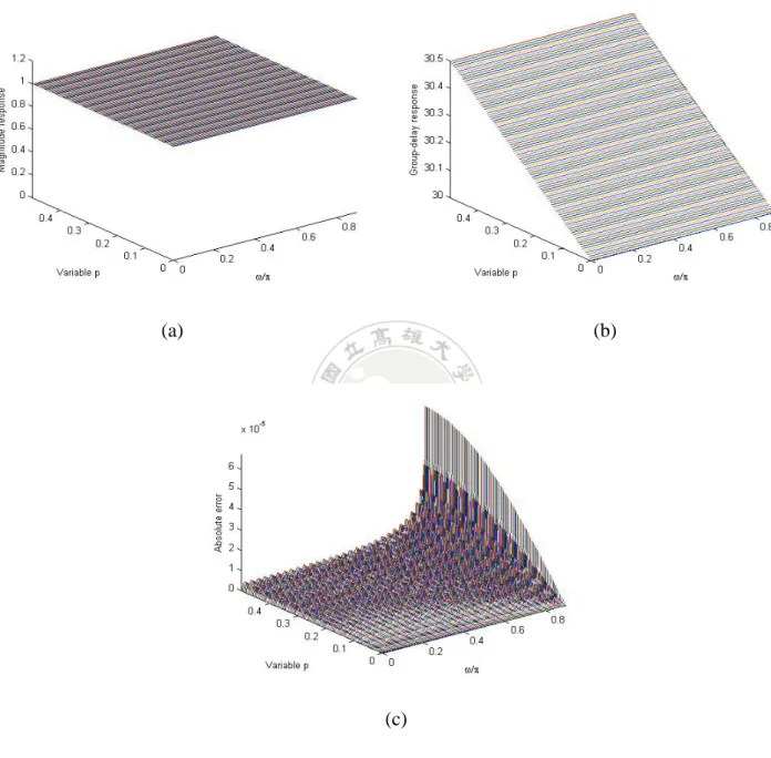
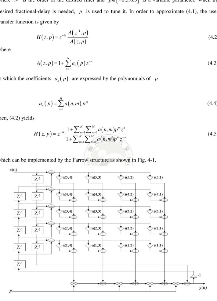
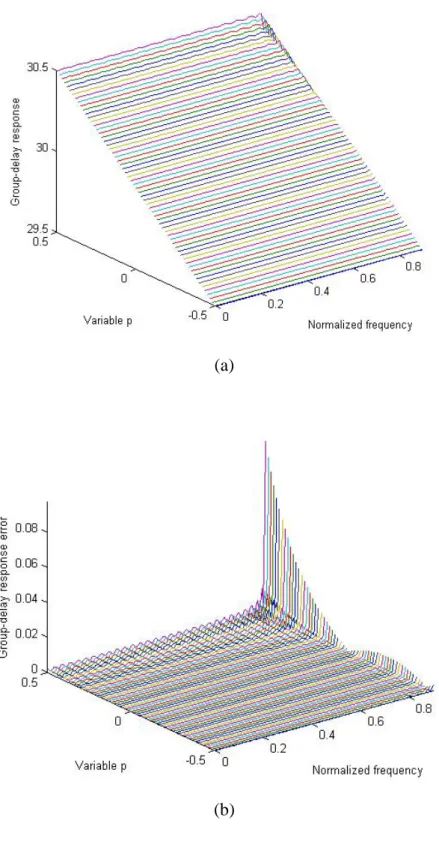
(25) ec ( x ) = ∫. 0.5. −0.5. xT PPT xdp = xT Qp x. (3.16). where Qp = ∫. 0.5. −0.5. PPT dp. (3.17). Then, the objective error function of the stable VFD IIR filter is gotten by e ( x ) = ea ( x ) + α ec ( x ) = s + xT r + xT Qx + α xQp x. (3.18). where α is a relative weighting constant. By differentiating (3.18) with respect to x and setting the result to zero can yield. x=−. 3.4. 1 (Q + α Q p ) r 2. (3.19). Numerical Examples. For example 1, it deals with the design of a N a = 14 , N b = 55 , M = 5 , ω p = 0.9π , I = 27 , VFD IIR filter. Fig. 3-2(a) presents the magnitude response. Fig. 3-2(b) displays the absolute error of variable frequency response. Besides, the group delay response and the absolute error of variable group-delay response are shown in Figs. 3-2(c) and (d), respectively. About example 2, a VFD IIR filter is designed with N a = N b = I = 35 , M = 5 , ω p = 0.9π , and W (ω ) = 1 . Figs. 3-3(a) and (b) illustrate the magnitude response and the absolute error of variable frequency response. The group-delay response is shown in Fig. 3-3(c). At last, the absolute error of variable group-delay response is presented in Fig. 3-3(d).. 15.

(26) (a). (b). (c). (d). Fig. 3-2 Design of a N a = 14 , N b = 55 , M = 5 , ω p = 0.9π , I = 27 VFD IIR filter. (a) Magnitude response (b) Absolute error of variable frequency response (c) Group-delay response (d) Absolute error of variable group-delay response.. 16.

(27) (a). (b). (c). (d). Fig. 3-3 D e s i g n o f a N a = N b = I = 3 5 , M = 5 , ω p = 0.9π , V F D I I R f i l t e r . (a) Magnitude response (b) Absolute error of variable frequency response (c) Group-delay response (d) Absolute error of variable group-delay response.. 17.

(28) 3.5 Conclusions. Weighted Least-Squares Approach was successfully used to design the VFD IIR filter in this chapter. To demonstrate the effectiveness of the proposed method, two design examples were presented. Notice that, the constrained value is needed to be less than 0.5 because of the stable condition must be satisfied. So, the stable problem of the VFD IIR filter can certainly be overcome. Finally, both the absolute error of variable frequency response and the absolute error of variable group-delay are significantly small.. 18.

(29) Chapter 4. Design of Variable Fractional-Delay Allpass Filters. 4.1 Introduction. In this chapter, the VFD Allpass filter is designed by Weighted Least-Squares Approach (WLS) method. As for the allpass filter design, the issue of stability is the principal problem [23]-[26]. However, the VFD Allpass filter would be stable if the variable parameter could be properly tuned between -0.5 and 0.5. In particular, each coefficient can be expressed as a polynomial-form, and all elements of relative vectors and matrices can be evaluated in closed-forms. First, the problem formulation is derived in section 4.2. Then, WLS method is introduced in section 4.3. Section 4.4 gives a VFD Allpass design example. Finally, some conclusions are offered in section 4.5. 4.2 Problem Formulation. As for the VFD Allpass filter, the desired response can be characterized by H d (ω , p ) = e − j ( N + p )ω , ω ≤ ω p. (4.1). 19.

(30) where N is the order of the desired filter and p ∈ [ −0.5, 0.5] is a variable parameter. When the desired fractional-delay is needed, p is used to tune it. In order to approximate (4.1), the used transfer function is given by H ( z, p ) = z. −N. A ( z −1 , p ). (4.2). A ( z, p ). where N. A ( z , p ) = 1 + ∑ an ( p ) z − n. (4.3). n =1. in which the coefficients an ( p ) are expressed by the polynomials of p. M. an ( p ) = ∑ a ( n, m ) p m. (4.4). n =1. then, (4.2) yields 1 + ∑ n =1 ∑ m =1 a ( n, m ) p m z n N. H ( z, p ) = z. −N. M. 1 + ∑ n =1 ∑ m =1 a ( n, m ) p m z − n N. M. which can be implemented by the Farrow structure as shown in Fig. 4-1.. Fig. 4-1 Farrow structure of an allpass VFD digital filter ( N = 5 , M = 4 ) 20. (4.5).

(31) According to (4.5), the frequency response would be express as. H (e , p) = e jω. − jN ω. A ( e − jω , p ). − jN ω. 1 + ∑ n =1 ∑ m =1 a ( n, m ) p m e jnω. A ( e jω , p ) N. =e. M. (4.6). 1 + ∑ n =1 ∑ m =1 a ( n, m ) p m e − jnω N. M. For the Allpass digital filter design, the problem only is focused on the phase approximation. Hence, the phase of (4.6). (. ). (. arg H ( e jω , p ) = − N ω − 2 arg A ( e jω , p ). ). (4.7). will approximate the phase of (4.1) arg ( H d (ω , p ) ) = − N ω − pω. (4.8). Therefore, the design problem can be expressed by. − tan. −1. ∑ ∑ a ( n, m ) p sin ( nω ) → pω , 2 1 + ∑ ∑ a ( n, m ) p cos ( nω ) N. M. n =1 N. m =1 M. n =1. m. m. 0 ≤ ω ≤ ω p , p1 ≤ p ≤ p1 + 1. (4.9). m =1. where “ → ” means “approximate”. Because of (4.9) is highly nonlinear, it can be converted into ⎛ pω ⎞ sin ⎜ ⎟ 2 ⎠ ⎛ pω ⎞ ⎝ − → tan ⎜ ⎟= N M ⎝ 2 ⎠ cos ⎛ pω ⎞ 1 + ∑ n =1 ∑ m =1 a ( n, m ) p m cos ( nω ) ⎜ ⎟ ⎝ 2 ⎠ 0 ≤ ω ≤ ω p , p1 ≤ p ≤ p1 + 1. ∑ n=1 ∑ m=1 a ( n, m ) p m sin ( nω ) N. M. (4.10). which can be further formulated into ⎛ pω ⎞ N M ⎛ pω ⎞ N M ⎛ pω ⎞ m m sin ⎜ , cos sin + a n m p n ω ( ) ( ) ⎟ ∑∑ ⎜ ⎟ + ∑∑ a ( n, m ) p sin ( nω ) cos ⎜ ⎟→0 ⎝ 2 ⎠ n =1 m =1 ⎝ 2 ⎠ n =1 m =1 ⎝ 2 ⎠ 0 ≤ ω ≤ ω p , p1 ≤ p ≤ p1 + 1. 21. (4.11).

(32) 4.3 Using Weighted Least-Squares Approach to design VFD Allpass filters. After previous discussion, the further analysis would be continued. By using Weighted Least-Squares Approach (WLS) method, the objective error function of the VFD Allpass filter can be represented by. e (a) = ∫ =∫. p1 +1. ∫. ωp. 0. p1 p1 +1. p1. ∫. ωp. 0. 2. ⎛ pω ⎞ N M ⎛ pω ⎞ ⎛ pω ⎞ ⎤ m ⎡ sin ⎜ ⎟ + ∑∑ a ( n, m ) p ⎢cos ( nω ) sin ⎜ ⎟ + sin ( nω ) cos ⎜ ⎟ ⎥ dω dp ⎝ 2 ⎠ n =1 m =1 ⎝ 2 ⎠ ⎝ 2 ⎠⎦ ⎣ 2. ⎛ pω ⎞ T sin ⎜ ⎟ + a c (ω , p ) dω dp ⎝ 2 ⎠. = s +rT a + aT Qa. where the superscript. (4.12). T. denotes the transpose operator,. a = ⎡⎣ a (1,1) , ⋅⋅⋅, a ( N ,1) , ⋅⋅⋅, a (1, M ) , ⋅⋅⋅, a ( N , M ) ⎤⎦. T. (4.13a ). ⎡ ⎛ ⎛ pω ⎞ ⎛ pω ⎞ ⎞ c (ω , p ) = ⎢ p ⎜ cos (ω ) sin ⎜ ⎟ + sin (ω ) cos ⎜ ⎟ ⎟ , ⋅⋅⋅, ⎝ 2 ⎠ ⎝ 2 ⎠⎠ ⎣ ⎝ ⎛ ⎛ pω ⎞ ⎛ pω ⎞ ⎞ p ⎜ cos ( N ω ) sin ⎜ ⎟ + sin ( N ω ) cos ⎜ ⎟ ⎟ , ⋅⋅⋅, ⎝ 2 ⎠ ⎝ 2 ⎠⎠ ⎝ ⎛ ⎛ pω ⎞ ⎛ pω ⎞ ⎞ p M ⎜ cos (ω ) sin ⎜ ⎟ + sin (ω ) cos ⎜ ⎟ ⎟ , ⋅⋅⋅, ⎝ 2 ⎠ ⎝ 2 ⎠⎠ ⎝ ⎛ ⎛ pω ⎞ ⎛ pω ⎞ ⎞ ⎤ p ⎜ cos ( N ω ) sin ⎜ ⎟ + sin ( N ω ) cos ⎜ ⎟ ⎟⎥ ⎝ 2 ⎠ ⎝ 2 ⎠ ⎠⎦ ⎝ M. T. (4.13b). and s=∫. p1 +1 p1. ∫. ωp. 0. ⎛ pω ⎞ sin 2 ⎜ ⎟dω dp ⎝ 2 ⎠. (4.14a ). 22.

(33) r = 2∫. Q=∫. p1 +1 p1. ωp. 0. p1 +1 p1. ∫. ⎛ pω ⎞ sin ⎜ ⎟c (ω , p ) dω dp ⎝ 2 ⎠. ωp. (4.14b). ∫ c (ω , p )c (ω , p ) dω dp T. (4.14c). 0. In order to solve to the solution, the error function e ( a ) is differentiated with respect to a and set the result to zero, which can obtain 1 a = − Q −1r 2. (4.15). Additionally, cos ( pω / 2 ) and sin ( pω / 2 ) are formulated by Taylor series expansion,. 2 k +1 ω p 2 k +1 1 ∞ ( −1) ( p1 + 1) − p1 s=− ∑ 2 k =1 ( 2k ) ! 2k + 1 2k + 1 2 k +1. k. (4.16a). and the elements of r and Q are gotten by − p1m + 2 k +1 ω 2 k ( −1) ( p1 + 1) × ∫ ω cos ( nω )dω r ( i ) = −∑ 0 m + 2k + 1 k =1 ( 2k ) ! k m+2k +2 ∞ −1) ( p1 + 1) − p1m + 2 k + 2 ω 2 k +1 ( +∑ × ∫ ω sin ( nω )dω 0 m + 2k + 2 k = 0 ( 2k + 1) ! m + 2 k +1. k. ∞. p. p. 0 ≤ i ≤ NM − 1. (4.16b). m + m +1 − p1m + mˆ +1 sin ( ( n − nˆ ) ω p ) 1 ( p1 + 1) Q ( i, l ) = m + mˆ + 1 n − nˆ 2 ˆ. − p1m + mˆ + 2 k +1 1 ∞ ( −1) ( p1 + 1) − ∑ m + mˆ + 2k + 1 2 k = 0 ( 2k ) ! m + mˆ + 2 k +1. k. ×∫ ω 2 k cos ( ( n + nˆ ) ω )d ω ωp. 0. − p1m + mˆ + 2 k + 2 1 ∞ ( −1) ( p1 + 1) + ∑ m + mˆ + 2k + 2 2 k =0 ( 2k + 1) ! k. m + mˆ + 2 k + 2. ×∫ ω 2 k +1 sin ( ( n + nˆ ) ω )dω ωp. 0 ≤ i, l ≤ NM − 1. 0. ⎢l ⎥ ⎢i ⎥ in which, n = mod ( i, N ) + 1 , m = ⎢ ⎥ + 1 , nˆ = mod ( l , N ) + 1 and mˆ = ⎢ ⎥ + 1 ⎣N ⎦ ⎣N ⎦ 23. (4.16c).

(34) Finally, s , r , and Q are approximated by sK , rK , Q K , respectively, − p12 k +1 ω p 2 k +1 1 K ( −1) ( p1 + 1) sK = − ∑ 2 k =1 ( 2k ) ! 2k + 1 2k + 1 2 k +1. k. (4.17 a). and −1) ( p1 + 1) − p1m + 2 k +1 ω 2 k ( × ∫ ω cos ( nω )dω rK ( i ) = −∑ 0 m + 2k + 1 k =1 ( 2k ) ! k m+2k +2 K −1) ( p1 + 1) − p1m + 2 k + 2 ω 2 k +1 ( +∑ × ∫ ω sin ( nω )dω 0 m + 2k + 2 k = 0 ( 2k + 1) ! m + 2 k +1. k. K. p. p. 0 ≤ i ≤ NM − 1. (4.17b). m + mˆ +1 − p1m + mˆ +1 sin ( ( n − nˆ ) ω p ) 1 ( p1 + 1) Q K ( i, l ) = m + mˆ + 1 n − nˆ 2. − p1m + mˆ + 2 k +1 1 K ( −1) ( p1 + 1) − ∑ m + mˆ + 2k + 1 2 k = 0 ( 2k ) ! m + mˆ + 2 k +1. k. ×∫ ω 2 k cos ( ( n + nˆ ) ω )dω ωp. 0. − p1m + mˆ + 2 k + 2 1 K ( −1) ( p1 + 1) + ∑ m + mˆ + 2k + 2 2 k =0 ( 2k + 1) ! k. m + mˆ + 2 k + 2. ×∫ ω 2 k +1 sin ( ( n + nˆ ) ω )d ω ωp. 0 ≤ i, l ≤ NM − 1. 0. 4.4. (4.17c). Numerical Example. In this example, an N = 30 , M = 5 , ω p = 0.9π , p ∈ [ −0.5, 0.5] allpass VFD filter is designed. Notice that, ω and p are uniformly sampled at step sizes ω p / 200 and 1/60. Fig. 4-2(a) displays the variable group-delay response. Then, the absolute group-delay error is illustrated in Fig. 4-2(b).. 24.

(35) (a). (b). Fig. 4-2 Design of an allpass VFD filter with N = 30 , M = 5 , ω p = 0.9π , p ∈ [ −0.5, 0.5] (a) Variable group-delay response (b) Absolute delay errors. 25.

(36) 4.5 Conclusions. The design of the VFD Allpass filter is summarized in this section. Weighted Least-Squares Approach (WLS) method was applied to achieve this design. Besides, the technique of Taylor series expansion was used such that all relative vectors and matrices can be calculated in closed-forms. Furthermore, the performance of the desired VFD Allpass filter would be obviously influenced because of the variable parameter p . It was also found that the variable parameter can be properly tuned to overcome the stability problem. At last, an example was offered to show the effectiveness of this proposed method.. 26.

(37) Chapter 5. Design of Variable Fractional-Order FIR Differintegrators. 5.1 Introduction. During the last decades, the concept of fractional calculus has been investigated in different aspects of engineering applications, such as electromagnetic theory, automatic control and signal processing [27]-[31]. Therefore, several methods have been developed for designing variable fractional-order differintegrators, integrators and differentiators [32]-[38]. Recently, this topic has been significant concerned and frequently discussed. Weighted Least-Squares Approach (WLS) can also be successfully applied to design the VFO FIR differintegrators, the pure VFO integrators and the pure VFO differentiators. In this chapter, the technique of WLS is proposed. The problem formulation is derived step by step in section 5.2. Then, section 5.3 provides some design examples to demonstrate the effectiveness. At last, the conclusions are given in section 5.4.. 5.2 Problem Formulation. For the design of the VFO differintegrator, the desired response is given by 27.

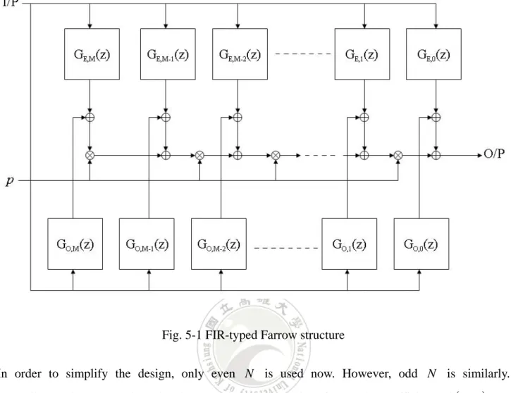
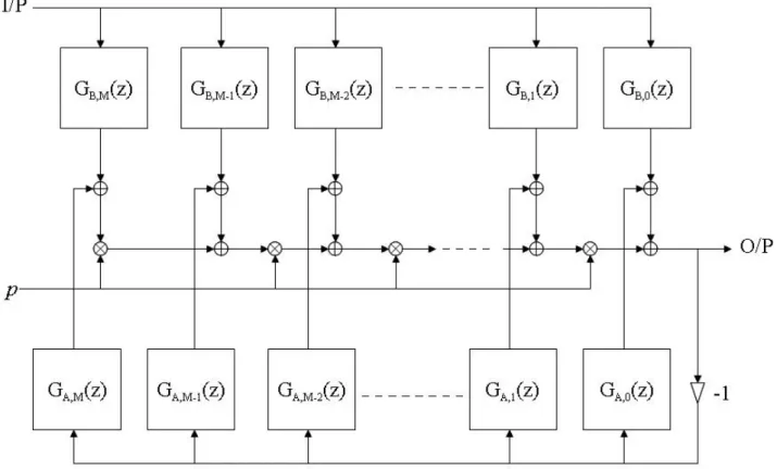
(38) D (ω , p ) = e − jI ω ( jω ) , p. ps ≤ p ≤ p f , ω s ≤ ω ≤ ω f. (5.1). where I is a prescribe delay and p is the variable order. When ps ≥ 0 and ωs ≥ 0 , it is a pure VFO differentiator. If p f ≤ 0 and ωs > 0 , it is a pure VFO integrator. As for ps < 0 < p f and. ωs > 0 , it is a VFO differintegrator. The subscripts s and. f. denotes the start points and final. points of the adjustable region and the designed band. Assume p Dˆ (ω , p ) = ( jω ) p ⎡ ⎛ pω ⎞ ⎛ pω ⎞ ⎤ = ω ⎢cos ⎜ ⎟ + j sgn (ω ) sin ⎜ ⎟⎥ ⎝ 2 ⎠⎦ ⎣ ⎝ 2 ⎠. (5.2). where sgn (.) means a sign function, then (5.1) can be rewritten as D (ω , p ) = e − jIω Dˆ (ω , p ). (5.3). In order to approach the desired response, the used transfer function is. N. H ( z , p ) = ∑ hn ( p ) z − n. (5.4). n =0. where the coefficients hn ( p ) are indicated as the polynomials of p. M. hn ( p ) = ∑ h ( n, m ) p m. (5.5). m =0. Substituting (5.5) into (5.4) can get N M M M ⎛ N ⎞ ⎛ N ⎞ H ( z , p ) = ∑∑ h ( n, m ) p m z − n = ∑ ⎜ ∑ he ( n, m )z − n ⎟ p m = ∑ ⎜ ∑ ho ( n, m )z − n ⎟ p m n =0 m =0 m =0 ⎝ n =0 m=0 ⎝ n =0 ⎠ ⎠ M. M. m =0. m=0. = ∑ GE , M ( z ) p m + ∑ GO , M ( z ) p m. 28. (5.6).

(39) Notice that, Eq. (5.6) can be implemented by FIR-typed Farrow structure as shown in Fig. 5-1.. Fig. 5-1 FIR-typed Farrow structure In order to simplify the design, only even N is used now. However, odd N is similarly. According to the symmetric and antisymmetric characteristics of (5.2), the coefficients h ( n, m ) are separated into even part and odd part by h ( n, m ) = he ( n, m ) + ho ( n, m ). (5.7). where ⎛N ⎞ 1⎡ ⎛N ⎞ ⎛N ⎞⎤ he ⎜ + n, m ⎟ = ⎢ h ⎜ + n, m ⎟ + h ⎜ − n, m ⎟ ⎥ ⎝2 ⎠ 2⎣ ⎝ 2 ⎠ ⎝2 ⎠⎦ N N − ≤n≤ , 0≤m≤M 2 2. (5.8a). and ⎛N ⎞ 1⎡ ⎛N ⎞ ⎛N ⎞⎤ ho ⎜ + n, m ⎟ = ⎢ h ⎜ + n, m ⎟ − h ⎜ − n, m ⎟ ⎥ ⎝2 ⎠ 2⎣ ⎝ 2 ⎠ ⎝2 ⎠⎦ N N − ≤n≤ , 0≤m≤M 2 2 29. (5.8b).

(40) As a result, the frequency response of the desired filter can be formulated into N /2 M ⎡ N /2 M ⎤ m a n , m p cos n ω j b ( n, m ) p m sin ( nω ) ⎥ + ( ) ( ) ∑∑ ∑∑ ⎢ n =1 m = 0 ⎣ n =0 m=0 ⎦ − j ( N /2 )ω ˆ H (ω , p ) =e. H ( e jω , p ) = e. − j ( N / 2 )ω. (5.9). where ⎧ ⎛N ⎞ ⎪he ⎜ 2 , m ⎟ ⎪ ⎝ ⎠ a ( n, m ) = ⎨ ⎪ 2 h ⎛ N − n, m ⎞ ⎟ ⎪⎩ e ⎜⎝ 2 ⎠. n = 0, 0 ≤ m ≤ M (5.10a ). N 1≤ n ≤ , 0 ≤ m ≤ M 2. ⎛N ⎞ b ( n, m ) = 2ho ⎜ − n, m ⎟ , ⎝2 ⎠. 1≤ n ≤. N , 0≤m≤M 2. (5.10b). and. N /2 M. Hˆ (ω , p ) = ∑∑ a ( n, m ) p m cos ( nω ) n =0 m=0. N /2 M. + j ∑ ∑ b ( n, m ) p m sin ( nω ). (5.11). n =1 m = 0. Obviously, I = N / 2 in (5.1) and (5.3). Let A be a. ( N / 2 + 1) × ( M + 1). matrix and B be a N / 2 × ( M + 1) matrix, respectively.. A and B are defined by. ⎡ A = ⎢ a ( n, m ) , ⎣. 0≤n≤. N ⎤ , 0≤m≤M⎥ 2 ⎦. (5.12a ). ⎡ B = ⎢b ( n, m ) , ⎣. 1≤ n ≤. N ⎤ , 0≤m≤M⎥ 2 ⎦. (5.12b). and. Moreover, the objective error function is used as below:. 30.

(41) Kω K p. (. e ( A, B ) = ∑∑ W (ωi ) D (ωi , pl ) − H e jωi , pl i =0 l =0. Kω K p. = ∑∑ W (ωi ) D (ωi , pl ) − Hˆ (ωi , pl ) i =0 l =0. ωi = ωs +. Based on a. i (ω f − ωs ). ( Kω + 1) × ( K p + 1). Kω. , pl = ps +. ). 2. 2. i ( p f − ps ). (5.13). Kp. grid, Kω = K p = 200 is used and W (ω ) is a positive weighting. function.. ⎡ ⎛ pπ e ( A, B ) = ∑∑ W (ωi ) ⎢ωi pl cos ⎜ l ⎝ 2 i =0 l =0 ⎣ Kω K p. ⎤ ⎞ N /2 M m ⎟ − ∑∑ a ( n, m ) pl cos ( nωi ) ⎥ ⎠ n =0 m =0 ⎦. ⎡ ⎛ pπ + ∑∑ W (ωi ) ⎢ωi pl sin ⎜ l ⎝ 2 i =0 l =0 ⎣ Kω K p. 2. ⎤ ⎞ N /2 M m ⎟ − ∑∑ b ( n, m ) pl sin ( nωi ) ⎥ ⎠ n =0 m =0 ⎦. 2. (5.14). Additionally, (5.14) can be expressed in matrix form as T T e ( A, B ) = tr ⎡⎢( DA − CAPT ) ( DA − CAPT ) ⎤⎥ + tr ⎡⎢( DB − SBPT ) ( DB − SBPT ) ⎤⎥ ⎣ ⎦ ⎣ ⎦ = e ( A) + e (B). where tr (.) denotes a trace operator, the superscript. T. (5.15). denotes a transpose operator,. ⎡ ⎛ pπ ⎞ DA = ⎢W 1/2 (ωi ) ωi pl cos ⎜ l ⎟ ⎝ 2 ⎠ ⎣. ⎤ 0 ≤ i ≤ Kω , 0 ≤ l ≤ K p ⎥ ⎦. (5.16a). ⎡ ⎛ pπ ⎞ DB = ⎢W 1/2 (ωi ) ωi pl sin ⎜ l ⎟ ⎝ 2 ⎠ ⎣. ⎤ 0 ≤ i ≤ Kω , 0 ≤ l ≤ K p ⎥ ⎦. (5.16b). ⎡ C = ⎢W 1/ 2 (ωi ) cos ( nωi ) ⎣. 0 ≤ i ≤ Kω , 0 ≤ n ≤. 31. N⎤ 2 ⎥⎦. (5.16c).

(42) ⎡ S = ⎢W 1/2 (ωi ) sin ( nωi ) ⎣ P = ⎡⎣ pl m. 0 ≤ i ≤ Kω , 1 ≤ n ≤. N⎤ 2 ⎥⎦. (5.16d ). 0 ≤ l ≤ K p , 0 ≤ m ≤ M ⎤⎦. (5.16e). and T e ( A ) = tr ⎡⎢( DA − CAPT ) ( DA − CAPT ) ⎤⎥ ⎣ ⎦ T T = tr ⎡⎢ DAT DA − DAT CAPT − ( CAPT ) D A + ( CAPT ) ( CAPT ) ⎤⎥ ⎣ ⎦. (5.17). T e ( B ) = tr ⎡⎢( DB − SBPT ) ( DB − SBPT ) ⎤⎥ ⎣ ⎦ T T = tr ⎡⎢ DBT DB − DBT SBPT − ( SBPT ) DB + ( SBPT ) ( SBPT ) ⎤⎥ ⎣ ⎦. (5.18). Differentiating e ( A, B ) with respect to A , ∂e ( A, B ) ∂e ( A ) = ∂A ∂A = − ( DAT C ). T. (P ). T T. − CT DA P + ( PAT CT C ). T. (P ). T T. + CT CAPT P. (5.19). Then set the result to zero, the coefficient matrix A can be gotten as A = ( CT C ) CT DA P ( PT P ) −1. −1. (5.20). The coefficient matrix B can also be gotten by the similar calculation as B = ( ST S ) ST D B P ( P T P ) −1. −1. (5.21). 32.

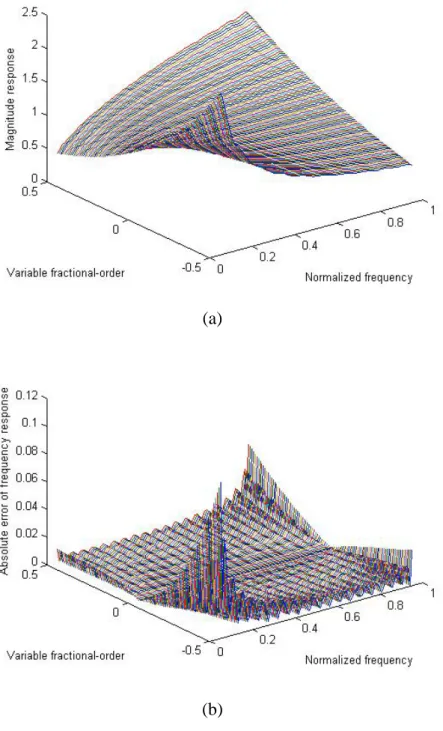
(43) 5.3 VFO FIR differintegrator, pure differentiator and pure integrator examples. The design example 1 deals with a VFO FIR differintegrator with N = 40 , M = 5 , ωs = 0.05π ,. ω f = 0.95π , ps = −0.5 , p f = 0.5 and W (ω ) = 1 . Figs. 5-2(a) and (b) display the variable magnitude response and the absolute error of variable frequency response, respectively. For example 2, a pure VFO differentiator is designed with N = 30 , M = 6 , ωs = 0 , ω f = 0.9π , ps = 1 , p f = 2 and W (ω ) = 1 . The variable magnitude response and the absolute error of variable frequency response are shown in Figs. 5-3(a) and (b). Then, consider the design of a VFO integrator with N = 60 , M = 6 , ωs = 0.05π , ω f = 0.9π , ps = −1.5 , and p f = −0.5 in the example 3. Similarly, Fig. 5-4(a) presents the variable magnitude response and Fig. 5-4(b) displays the absolute error of variable frequency response. Notice that, this technique can also be applied when N is odd.. 33.

(44) (a). (b). Fig. 5-2 Design of a VFO differintegrator with N = 40 , M = 5 , ωs = 0.05π , ω f = 0.95π , ps = −0.5 , and p f = 0.5 (a) Variable magnitude response (b) Absolute error of variable frequency response.. 34.

(45) (a). (b). Fig. 5-3 Design of a VFO differentiator with N = 30 , M = 6 , ωs = 0 , ω f = 0.9π , ps = 1 , and p f = 2 (a) Variable magnitude response (b) Absolute error of variable frequency response.. 35.

(46) (a). (b). Fig. 5-4 Design of a VFO integrator with N = 60 , M = 6 , ωs = 0.05π , ω f = 0.9π , ps = −1.5 , and p f = −0.5 (a) Variable magnitude response (b) Absolute error of variable frequency response.. 36.

(47) 5.4 Conclusions. In this section, the design of the variable fractional-order FIR differintegrators is summarized. The technique of Weighted Least-Squares Approach was proposed for designing the VFO FIR differintegrators. Besides, the symmetric and antisymmetric characteristics were also applied to the coefficients of the VFO FIR filters. As a result, not only even N but also odd N can be used by this method. Finally, some design examples, including a VFO FIR differintegrator, a pure VFO differentiators and a pure VFO integrator, were presented to demonstrate the design effectiveness.. 37.

(48) Chapter 6. Design of Variable Fractional-Order IIR Differintegrators. 6.1 Introduction. In this chapter, the design of the VFO IIR differintegrators based on IIR-typed Farrow structure is proposed. For designing the IIR digital filters, the issue of the stability is significant concerned [39]-[40]. By incorporating a constrained function into the objective error function, the stability of the VFO IIR digital filters can be overcome. To achieve the results which satisfy the stable condition and simplify the calculations, a quadratic method is successfully used to deal with this highly nonlinear problem [41]. This chapter is organized as follows: problem formulation is derived step by step in section 6.2. Section 6.3 gives three examples, containing a VFO IIR differintegrator, a pure VFO IIR differentiator, and a pure VFO IIR integrator. At last, the conclusions are summarized in section 6.4.. 6.2 Problem Formulation. For designing the VFO differintegrator, the desired response is given by. 38.

(49) p H d (ω , p ) = e − jIω ( jω ) = e − jIω Hˆ d (ω , p ). ps ≤ p ≤ p f , ω s ≤ ω ≤ ω f. (6.1). where I is a prescribed delay and p is the variable order. If ps ≥ 0 and ωs ≥ 0 , it is a pure VFO differentiator. When p f ≤ 0 and ωs > 0 , it is a pure VFO integrator. As for ps < 0 < p f and. ωs > 0 , it is a VFO differintegrator. The subscripts s and. f. denotes the start points and final. points of the adjustable region and the designed band. Let p ⎡ ⎛ pω ⎞ ⎛ pω ⎞ ⎤ Hˆ d (ω , p ) = ω ⎢cos ⎜ ⎟ + j sgn (ω ) sin ⎜ ⎟⎥ ⎝ 2 ⎠⎦ ⎣ ⎝ 2 ⎠. (6.2). where sgn (.) means a sign function. To approximate the desired response, the used transfer function of VFO IIR filter is b b ( p ) z −n B ( z, p ) ∑ n =0 n H ( z, p ) = = A ( z , p ) 1 + ∑ N a an ( p ) z − n n =1. N. (6.3). where the coefficients an ( p ) and bn ( p ) are indicated as the polynomials of p. M. an ( p ) = ∑ a ( n, m ) p m , m=0. M. bn ( p ) = ∑ b ( n, m ) p m , m=0. 1 ≤ n ≤ Na. (6.4a). 0 ≤ n ≤ Nb. (6.4b). Substituting (6.4a) and (6.4b) into (6.3) can yield. ∑ ∑ b ( n, m ) p z H ( z, p ) = 1 + ∑ ∑ a ( n, m ) p z. m −n. Nb. M. n =0 Na. m=0 M. n =1. m =0. ∑ = 1+ ∑ M. m −n. in which 39. m=0 M. GB , m ( z ) p m. G ( z ) pm m = 0 A, m. (6.5).

(50) Na. G A , m ( z ) = ∑ a ( n, m ) z − n. 0≤m≤M. (6.6a ). 0≤m≤M. (6.6b). n =1. Nb. GB , m ( z ) = ∑ b ( n, m ) z − n n =0. Notice that, (6.5) can be implemented by IIR-typed Farrow structure as shown in Fig. 6-1.. Fig. 6-1 IIR-typed Farrow structure As a result, the frequency response of the desired filter can be formulated into. b ( n, m ) p e ω ∑ ∑ H (e , p) = 1 + ∑ ∑ a ( n, m ) p e ω jω. m − jn. Nb. M. n=0 Na. m =0 M. n =1. m − jn. m=0. bT c b ( ω , p ) − jbT s b ( ω , p ) = 1 + aT ca (ω , p ) − jaT sa (ω , p ). where the superscript. T. denotes a transpose operator, 40. (6.7).

(51) a = ⎣⎡ a (1, 0 ) ,..., a ( N a , 0 ) ,..., a (1, M ) ,..., a ( N a , M ) ⎦⎤. T. (6.8a). c a (ω , p ) = ⎡⎣cos (ω ) ,..., cos ( N aω ) ,..., p M cos (ω ) ,..., p M cos ( N aω ) ⎤⎦ s a (ω , p ) = ⎡⎣sin (ω ) ,...,sin ( N aω ) ,..., p M sin (ω ) ,..., p M sin ( N aω ) ⎤⎦. T. (6.8b). T. (6.8c). and b = ⎡⎣b ( 0, 0 ) ,..., b ( N a , 0 ) ,..., b ( 0, M ) ,..., b ( N a , M ) ⎦⎤ cb (ω , p ) = ⎡⎣1,..., cos ( N bω ) ,..., p M ,..., p M cos ( N bω ) ⎤⎦ sb (ω , p ) = ⎡⎣ 0,...,sin ( N bω ) ,..., 0,..., p M sin ( N bω ) ⎤⎦. T. (6.8d ). T. (6.8e). T. (6.8 f ). Thus, the approximation error function can be gotten by em ( a, b ) = ∫ =∫. pf ps. ωf. pf. ∫ω. ps. s. ωf. ∫ω. s. H d (ω , p ) − H ( e jω , p ) d ω dp. T T pπ ⎞ pπ ⎞ b cb (ω , p ) − jb sb (ω , p ) ⎛ ⎛ p ω cos ⎜ I ω − − j ω sin I ω − − dω dp ⎟ ⎜ ⎟ 2 ⎠ 2 ⎠ 1 + aT c a (ω , p ) − jaT s a (ω , p ) ⎝ ⎝ 2. p. (6.9). Concerning the stability of the VFO IIR digital filter, it has been shown in [41] that. Na. Na. n =1. n =1. 1 + ∑ an ( p ) cos ( nω ) ≥ 1 − 2∑ an 2 ( p ). when of. ∑. ∑ Na n =1. Na n =1. (6.10). an2 ( p ) is less than 0.5, the desired filter is stable for the specified p . Hence, the value. an2 ( p ) must be small enough to satisfy the stable condition. The constrained function is. defined by. 41.

(52) ⎛ Na 2 ⎞ ec ( a ) = ∫ ⎜ ∑ an ( p ) ⎟dp ps ⎝ n =1 ⎠ 2 N ⎞ pf ⎛ a ⎛ M m⎞ = ∫ ⎜ ∑ ⎜ ∑ a ( n, m ) p ⎟ ⎟dp ps ⎜ ⎠ ⎟⎠ ⎝ n =1 ⎝ m =0 pf. (6.11). Therefore, the objective error function of the VFO IIR digital filter can be given by e ( a,b ) = em ( a,b ) + α ec ( a ) =∫. pf ps. ⎛ ⎝. ωf. ∫ω. ω p cos ⎜ I ω −. s. pπ 2. pπ ⎞ ⎞ ⎛ p ⎟ − jω sin ⎜ I ω − ⎟ 2 ⎠ ⎠ ⎝. bT c b ( ω , p ) − jbT s b ( ω , p ) − d ω dp 1 + a T c a ( ω , p ) − ja T s a ( ω , p ) 2 N pf ⎛ a ⎛ M ⎞ ⎞ +α ∫ ⎜ ∑ ⎜ ∑ a ( n, m ) p m ⎟ ⎟dp ps ⎜ ⎠ ⎟⎠ ⎝ n =1 ⎝ m =0. (6.12). where α is a relative weighting constant. To simplify the calculation, the objective error function is expressed as ek ( a k , b k ) = em ,k ( a k , b k ) + α ec ,k ( a k ) =∫. ωf. pf. ∫ω. ps. s. ⎛ p pπ ⎞ ⎛ ω cos ⎜ I ω − ⎟ ⎜ A (ω , p ) ⎝ 2 ⎠ ⎝ 1. 2 k −1. pπ ⎞ ⎞ ⎛ T − jω p sin ⎜ I ω − ⎟ ⎟ (1 + a k c a (ω , p ) 2 ⎠⎠ ⎝ − jaTk s a (ω , p ) ) − ( bTk cb (ω , p ) − jbTk sb (ω , p ) ) d ω dp 2. +α ∫. pf ps. 2 ⎛ Na ⎛ M ⎞ m⎞ ⎜ ∑ ⎜ ∑ ak ( n, m ) p ⎟ ⎟dp ⎜ n =1 ⎝ m =0 ⎠ ⎟⎠ ⎝. (6.13). in which Ak −1 (ω , p ) = 1 + aTk −1c a (ω , p ) − jaTk −1s a (ω , p ) 2 2 = ⎡⎢(1 + aTk −1c a (ω , p ) ) + ( aTk −1s a (ω , p ) ) ⎤⎥ ⎣ ⎦. Moreover, defining. 42. 0.5. (6.14).

(53) ⎡a k ⎤ xk = ⎢ ⎥ ⎣b k ⎦. (6.15a). ⎡ p pπ ⎞ pπ ⎞ ⎤ ⎛ ⎛ p ⎢ω cos ⎜ I ω − 2 ⎟ c a (ω , p ) − ω sin ⎜ I ω − 2 ⎟ s a (ω , p ) ⎥ c (ω , p ) = ⎢ ⎝ ⎠ ⎝ ⎠ ⎥ ⎢⎣ ⎥⎦ −c b ( ω , p ). (6.15b). ⎡ p pπ ⎞ pπ ⎞ ⎤ ⎛ ⎛ p ⎢ω sin ⎜ I ω − 2 ⎟ c a (ω , p ) + ω cos ⎜ I ω − 2 ⎟ s a (ω , p ) ⎥ s (ω , p ) = ⎢ ⎝ ⎠ ⎝ ⎠ ⎥ ⎢⎣ ⎥⎦ −sb (ω , p ). (6.15c). and. Then, (6.13) becomes 2 ⎛⎡ p pπ ⎞ T ⎤ ⎛ em ,k ( x k ) = ∫ ∫ ⎜ ⎢ω cos ⎜ I ω − ⎟ + x k c (ω , p ) ⎥ ps ω s A 2 ⎜ 2 ⎠ ⎝ ⎦ k −1 ( ω , p ) ⎝ ⎣ 2 pπ ⎞ T ⎡ p ⎤ ⎞ ⎛ + ⎢ω sin ⎜ I ω − ⎟ + x k s (ω , p ) ⎥ ⎟⎟ d ω dp 2 ⎠ ⎝ ⎣ ⎦ ⎠ = s + xTk r + xTk Qx k. ωf. pf. 1. (6.16). where. pf. s=∫. ps. r=∫. pf ps. ωf. ∫ω. s. ωf. ∫ω. s. 1. 2 k −1. A. ω 2 p dω dp. (6.17 a). (ω , p ). ⎡ p pπ ⎞ ⎛ 2ω cos ⎜ I ω − ⎟c (ω , p ) ⎢ A (ω , p ) ⎣ 2 ⎠ ⎝ 1. 2 k −1. pπ ⎞ ⎤ ⎛ + 2ω p sin ⎜ I ω − ⎟ s (ω , p ) ⎥ dω dp 2 ⎠ ⎝ ⎦ Q=∫. pf ps. ωf. ∫ω. s. 1. ⎡⎣c (ω , p ) cT (ω , p ) + s (ω , p ) sT (ω , p ) ⎤⎦ d ω dp A (ω , p ) 2 k −1. Additionally, the integrand of the constrained function can be formulated into. 43. (6.17b). (6.17c).

(54) 2. ⎛ M m⎞ T T ∑ ⎜ ∑ ak ( n, m ) p ⎟ = x k PP x k n =1 ⎝ m = 0 ⎠ Na. (6.18). where. P = ⎡⎣ I Na , pI Na ,..., p M I N a , 0 ⎤⎦. T. (6.19). in which I Na is an N a × N a identity matrix and 0 means a N a × ( N b + 1)( M + 1) zero matrix. Significantly, the constrained function would become ec , k ( x k ) = ∫ xTk PPT x k dp = xTk Q p x k pf. (6.20). ps. where. pf. Q p = ∫ PPT dp. (6.21). ps. So the original nonlinear problem in (6.12) can be converted into a quadratic problem, and the objective error function is indicated as ek ( x k ) = em ,k ( x k ) + α ec , k ( x k ) = s + xTk r + xTk Qx k + α xTk Q p x k. (6.22). Furthermore, by differentiating e ( x k ) with respect to x k , and setting the result to zero, the solution can be obtained as below:. xk = −. −1 1 Q + αQ p ) r ( 2. (6.23). Importantly, the coefficients of the VFO IIR differintegrator design is. 44. ( N a + Nb + 1)( M + 1) ..

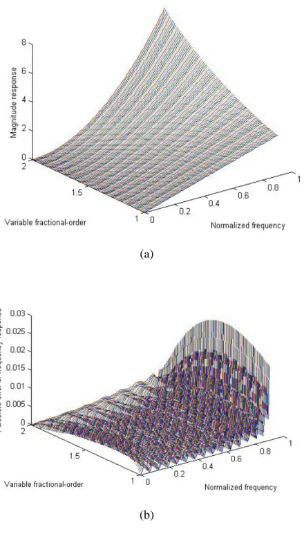
(55) 6.3 VFO FIR differintegrator, pure differentiator and pure integrator examples. Three examples are designed in this section. For example 1, it deals with a VFO IIR differintegrator with I = 19 , N a = 11 , N b = 29 , M = 5 , ωs = 0.05π , ω f = 0.95π , ps = −0.5 and p f = 0.5 , and shows the results in Figs. 6-2(a) and (b), which are the magnitude response and absolute error of variable frequency response. A pure VFO IIR differentiator with I = 14 , N a = 7 , N b = 23 , M = 3 , ωs = 0 , ω f = 0.9π , ps = 1 and p f = 2 is designed in the example 2. Fig. 6-3(a) presents the magnitude response of a pure VFO IIR differentiator. Besides, Fig. 6-3(b) displays the absolute error of variable frequency response. Then, consider the design of a pure VFO IIR integrator with I = 28 , N a = 15 , N b = 45 , M = 4 , ωs = 0.05π , ω f = 0.9π , ps = −1.5 , and p f = −0.5 in the example 3. Similarly, the magnitude response and the absolute error of variable frequency response of a pure VFO IIR integrator are illustrated in Figs. 6-4(a) and (b).. 45.

(56) (a). (b). Fig. 6-2 Design of a N a = 11 , N b = 29 , M = 5 , ωs = 0.05π , ω f = 0.95π , ps = −0.5 , p f = 0.5 , α = 1.77827294 × 10 −5 and I = 19 VFO IIR differintegrator. (a) Magnitude response (b) Absolute error of variable frequency response.. 46.

(57) (a). (b). Fig. 6-3 Design of a N a = 7 , N b = 23 , M = 3 , ωs = 0 , ω f = 0.9π , ps = 1 , p f = 2 ,. α = 1.77827294 × 10−4 and I = 14 VFO IIR differentiator (a) Magnitude response (b) Absolute error of variable frequency response.. 47.

(58) (a). (b). Fig. 6-4 Design of a N a = 15 , Nb = 45 , M = 4 , ωs = 0.05π , ω f = 0.9π , ps = −1.5 , p f = −0.5 , α = 5.62341325 ×10−2 and I = 28 VFO IIR integrator (a) Magnitude response (b) Absolute error of variable frequency response.. 48.

(59) 6.4 Conclusions. The design of the VFO IIR differintegrator, including the pure VFO IIR differentiator and the pure VFO IIR integrator, is summarized in this section. To implement it, IIR-typed Farrow structure was proposed. A quadratic method was used to overcome the highly nonlinear problem of the objective error function and simplify the calculations. However, the relative weighting constant α was different in all design examples because it must be properly chosen in order to ensure the stability of the designed filters. To show the performance, three examples were presented. In these three examples, the frequency ω and the variable parameter p were sampled similarly, which were. (ω. f. − ωs ) / 200 and. (p. f. − ps ) / 200 , respectively. Finally, the results of this method are illustrated. in Figs. 6-2, 6-3, and 6-4.. 49.

(60) Chapter 7 Conclusions and Future works. In this thesis, it is focused on investigating the various designs of variable digital filters. These designs are all discussed in detail. First, the research topic is concentrated on the variable fractional-delay (VFD) filters. The VFD FIR, VFD IIR, and VFD Allpass filters are designed in chapters 2, 3, and 4. Weighted Least-Squares Approach (WLS) has been successfully used to achieve the desired results, including the magnitude response, the group-delay response, the absolute error of variable frequency response, and the absolute group-delay error. As for the IIR and Allpass filters, they are more difficult to realize than the FIR filters because their stability problem must be considerable attention. Fortunately, the desired VFD filter systems can be implemented by the Farrow structure. Second, the variable fractional-order (VFO) differintegrators are also concerned. The VFO FIR differintegrators and the VFO IIR differintegrators are proposed to design in chapters 5 and 6, respectively. Besides, both the pure VFO differentiator and the pure VFO integrator can be realized by choosing the proper range of the parameter p . Similarly, the results can be obtained to demonstrate the performance as well. In addition, the VFO IIR differintegrators also must satisfy the stable condition. In the design procedure of this thesis, many techniques are applied to achieve the desired goals. Binomial Series Expansion and Taylor Series Expansion helpfully evaluate the related vectors or matrices in closed-forms. The symmetric or antisymmetric relationships of the filter coefficients are also widely used. When the highly nonlinear formulations occur, quadratic method can overcome them to simplify the calculations and complexity. In the future, the research of the variable digital filters will be more developed due to their wide applications. Based on many past achievements in regard to this aspect, more and more methods and criteria will appear. So, this issue is still worthy of further study.. 50.

(61) Reference [1] S.-C. Pei and C.-C. Tseng, “A comb filter design using fractional-sample delay”, IEEE Trans.Circuits Syst. I, Analog Digit. Signal Process., vol. 45, pp. 649-653, June 1998.. [2] R. Sobot, S. Stapleton and M. Syrzycki, “Tunable continuous-time bandpass ∑ Δ modulators with fractional delays”, IEEE Trans. Circuits Syst. I, Reg. Papers, vol. 53, pp. 264-273, Feb. 2006. [3] K.-J. Cho, J.-S. Park, B.-K. Kim, J.-G. Chung and K. K. Parhi, “Design of a sample-rate converter from CD to DAT using fractional delay allpass filter”, IEEE Trans. Circuits Syst. II, Exp. Brief, vol. 54, pp. 19-23, Jan. 2007. [4] H.-M. Lehtonen, V. Valimaki and T. I. Laakso, “Canceling and selecting partials from musical tones using fractional-delay filters”, Computer Music Journal, vol. 32, pp. 43-56, Feb. 2008. [5] C. W. Farrow, “A continuously variable digital delay element”, in Proc. ISCAS, 1998, pp. 2641-2645. [6] C.-C. Tseng, “Design and applications of variable fractional order differentiator”, in IEEE Asia-Pacific Conference on Circuits and Systems, Dec. 2004, pp. 405-408. [7] Y.Q. Chen and B.M. Vinagre, “A new IIR-type digital fractional order differentiator”, Signal Processing, vol. 83, pp. 2359-2365, 2003. [8] P. Ostalczyk, “Fundamental properties of the fractional-order discrete-time integrator”, Signal Processing, vol.83, pp. 2367-2376, 2003. [9] Y.Q. Chen and K.L. Moore, “Discretization schemes for fractional-order differentiators and integrators”, IEEE Trans. Circuits Syst. I, vol. 49, pp. 363-367, Mar. 2002. [10] C.-C. Tseng, “Design of variable and adaptive fractional order differentiators”, Signal Processing, vol. 86, pp. 2554-2566, 2006. [11] H. Zhao, G. Qin, L. Yao and J. Yu, “Design of fractional order digital FIR differentiators using frequency response approximation”, in Proceedings of the 2005 International Conference on Communications, Circuits and Systems, May 2005, pp. 1318-1321.. 51.

(62) [12] G. Maione, “Concerning continued fraction representation of nonlinear order digital differentiators”, IEEE Signal Process. Lett., vol. 13, pp. 725-728, Dec. 2006. [13] D. Xue, C. Zhao and Y.Q. Chen, “A modified approximation method of fractional order system”, in Proceeding of the 2006 IEEE International Conference on Mechatronics and Automation, June 2006, pp. 1043-1048. [14] T.-B. Deng, “Symmetric structures for odd-order maximally flat and weighted-least-squares variable fractional-delay filters”, IEEE Trans. Circuit Syst. I. Reg. Papers, vol.54, no.12, pp. 2718-2732, Dec. 2007. [15] J.-C. Liu and S.-J. You, “Weighted least squares near-equiripple approximation of variable fractional delay FIR filters”, IET Signal Process., vol.1, no.2, pp. 66-72, 2007. [16] C.Y. Chi and Y.T. Kou, “A new self-initiated optimum WLS approximation method for the design of linear phase FIR digital filters”, in Proc. ISCAS, 1991, pp. 168-171. [17] T.-B. Deng, “High-resolution image interpolation using two-dimensional Lagrange-type variable fractional-delay filter,” in IEICE Technical Report, Hirosaki, Japan, Mar. 2005, vol. SIS2004-60, pp. 27–30. [18] C.-C. Tseng, “Design of variable fractional delay FIR filters using symmetry”, in Proc. 2004 IEEE Int. Symp. Circuits and Systems, Vancouver, Canada, May 23–26, 2004, vol. III, pp. 477–480. [19] M. O. Ahmad and J.-D. Wang, “An analytical least square solution to the design problem of two-dimensional FIR filters with quadrantally symmetric or antisymmetric frequency response”, IEEE Trans. Circuits Syst., vol. 36, no. 7, pp. 968-979, Jul. 1989. [20] T.-B. Deng and Y. Lian, “Weighted-least-squares design of variable fractional-delay FIR filters using coefficient symmetry”, IEEE Trans. Signal Process., vol. 54, no. 8, pp . 3023-3038, Aug. 2006. [21] H. Zhao, H.K. Kwan, L. Wan and L. Nie, “Design of 1-D stable variable fractional delay IIR filters using finite impulse response fitting”, in Proc. ICCCAS, 2006, pp. 201-205. [22] H. Zhao and H.K. Kwan, “Design of 1-D stable variable fractional delay IIR filters”, IEEE Trans. Circuit Syst. II, Exp. Briefs, vol. 54, pp. 86-90, Jan. 2007. [23] K. Rajamani and Y.-S. Lai, “A novel method for designing allpass digital filters”, IEEE Signal Processing Letters, vol. 6, pp. 207-209, Aug. 1999. [24] W.R. Lee, L. Caccetta and V. Rehbock, “Optimal design of all-pass variable fractional-delay digital filters”, IEEE Transactions on Circuits Systems I, Regular Papers, vol. 55, pp. 1248-1256, May 2008.. 52.

(63) [25] J.-J. Shyu and S.-C. Pei, “A new approach to the design of complex allpass IIR digital filters”, Signal Processing, vol.40, pp. 207-215, Sep. 1994. [26] S.-C. Pei and P.-H. Wang “Closed-form design of all-pass fractional delay filters”, IEEE Signal Processing Letters, vol. 11 pp. 788-791, Oct. 2004. [27] B. Mbodje and G. Montseny, “Boundary fractional derivative control of the wave equation”, IEEE Trans. Automat. Control, vol. 40, pp. 378-382, Feb. 1995. [28] N. Engheta, “On fractional calculus and fractional multipoles in electromagnetism”, IEEE Trans. Antennas Propag., vol. 44, pp.554-556, Apr. 1996. [29] R. Hilfer (Ed.), “Application of Fractional Calculus in Physics”, World Scientific, River Edge, NJ, 2000. [30] B.M. Vinagre, I. podlubny, A. Hernandez and V. Feliu, “Some approximation of fractional order operators used in control theory and applications”, J.Fractional Calculus Appl. Anal., vol. 4, pp.47-66, 2001. [31] B.Mathieu, P. Melchior, A. Ousaloup and C. Ceyral, “Fractional differentiation for edge detection”, Signal Processing, vol. 83, pp. 2421-2432, 2003. [32] C.-C. Tseng, “Design of fractional order digital FIR differentiators”, IEEE Signal Process. Lett., vol. 8, pp. 77-79, Mar. 2001. [33] S. Samadi, M.O. Ahmad and M.N.S. Swamy, “Exact fractional-order differentiators for polynomial signals”, IEEE Signal Process. Lett., vol. 11, pp. 529-532, June, 2004. [34] C.-C. Tseng, “Improved design of digital fractional-order differentiators using fractional sample delay”, IEEE Trans. Circuits Systems I, vol. 53, pp. 193-203, Jan. 2006. [35] C.-C. Tseng, “Design of FIR and IIR fractional order Simpson digital integrators”, Signal Processing, vol. 87, pp. 1045-1057, 2007. [36] C.K.S. Pun, S.C. Chan, K.S. Yeung and K.L. Ho, “On the design and implementation of FIR and IIR digital filters with variable frequency characteristics”, IEEE Trans. Circuits Systems II, vol. 49, pp. 689-703, Nov. 2002. [37] T.-B. Deng, “Design of arbitrary-phase variable digital filters using SVD-based vector-array decomposition”, IEEE Trans. Circuits Systems I, vol. 52, pp. 148-167, Jan. 2005. [38] T.I. Laakso, V. Valimaki, M. Karjalainen and U.K. Laine, “Splitting the unit delay: tools for fractional delay filter design”, IEEE Signal Process. Mag., vol.13, pp. 30-60, 1996. [39] M. Makundi, T.I. Laakso and V. Valimaki, “Efficient tunable IIR and allpass filter structures”, Electronics Lett., vol. 37, pp. 344-345, June 2001. [40] H. Zhao and H.K. Kwan, “Design of 1-D stable variable fractional delay IIR filters”, in Proc. IEEE ISPACS, 2005, pp. 517-520. 53.