基於約略集合之藥物不良反應信號偵測方法於具缺漏值之通報資料的可行性研究

全文

(1)國立高雄大學資訊工程學系(研究所) 碩士論文. 基於約略集合之藥物不良反應信號偵測方法於具缺漏值之通報資料的可行性研究 On the Feasibility of Rough-Set-based ADR Signaling from Spontaneous Reporting Data with Missing Values. 研究生：藍琳撰指導教授：林文揚博士. 中華民國 103 年 7 月.

(2) 致謝. 感謝我的指導教授林文揚，在做研究的這段期間，給予我許多研究方面的意見和討論研究上所遇到的問題。藉由每次的討論結果，讓我學習到許多知識，也藉由這次的研究，提升自我的實作能力。感謝洪宗貝教授和王學亮教授，藉由每次論文報告，學習到許多報告技巧和做簡報的能力。另外也要感謝所有在研究所這段期間，給予我幫助的同學和老師，每當我遇到困難時，藉由討論和聊天中得到一些靈感。最後我要感謝我的家人，謝謝他們給予我許多支持和鼓勵，提供我一個安靜且舒適的環境做研究，讓我得以專心的完成我的研究。. i.

(3) 基於約略集合之藥物不良反應信號偵測方法於具缺漏值之通報資料的可行性研究. 指導教授：林文揚博士（教授）國立高雄大學資訊工程學系(研究所) 學生：藍琳國立高雄大學資訊工程學系(研究所) 摘要. 藥物不良反應係指在正常用藥劑量下所引起的有害的反應(副作用)；嚴重的藥物不良反應甚至會導致病人死亡或威脅生命的後果。由於有相當多的不良反應無法在有限的臨床試驗被發現，許多先進國家乃建置自發性通報系統，盡可能地收集所有的不良反應事件，以監控上市的藥物並發掘可能的不良反應。不幸地，由於隱私問題或其他原因，通報者有時故意漏填某些欄位，造成這些通報資料含有許多的缺漏資料。這些缺漏資料多少會影響分析結果，導致結果產生偏差。大多數的不良反應偵測的研究或實際採用的作法皆採用刪除法，直接刪掉含有缺漏值的資料。目前仍未見有研究注意到並進而研究，在進行不良反應偵測的過程中將這些缺漏納入考量是否可行且效果如何的問題。本論文可視為是探索此問題的先期性的研究。我們目標在探討使用約略集合論於藥物不良反應偵測的可行性。我們提出使用基於特徵集合的估算，來計算不良反應信號的強度。我們提出了 12 種不同的計算方法，並且使用我們提出的兩個新的觀念，滿足性及不可分辨性，證明其中只有六種方法是適合的計算方法。經由我們使用美國食品藥物管理局(FDA)的藥物不良反應通報系統的資料所進行的實驗顯示，我們提出的方法具有和傳統的方法相似的可疑不良反應信號的定期預警能力，而且對於某些已知的不良反應，我們的方法可以產生高於門檻的信 ii.

(4) 號強度值，而傳統的方法卻無法產生預期的信號。我們的研究顯示，利用約略集合理論可以將缺漏值納入不良反應信號的強度計算，且能弭補傳統的方法的不足處，因此可作為一種輔助的方法。. 關鍵字：藥物不良反應、列聯表、缺漏值、藥物安全監測、約略集合論、自發性通報資料. iii.

(5) On the Feasibility of Rough-Set-based ADR Signaling from Spontaneous Reporting Data with Missing Values. Advisor(s): Dr. (Professor) Wen-Yang Lin Institute of Computer Science and Information Engineering National University of Kaohsiung Student: Lin Lan Institute of Computer Science and Information Engineering National University of Kaohsiung ABSTRACT. Adverse Drug Reactions (ADRs) are uncomfortable or harmful reactions (side effects) in normal doses of drug usage; serious ADRs may even lead to death or lifethreatening outcomes of patients. Since many ADRs cannot be disclosed through limited clinical trials, most of the developed countries have established spontaneous reporting systems to collect as could as possible all adverse drug events in order to monitor the marketed drugs and to discover suspicious ADR signals. Unfortunately, due to privacy concern or other reasons, the reporters sometimes may omit consciously some attributes, causing many missing values existing in the reporting database. These missing data can reduce the accuracy of results for data analysis. Most of published research work on ADR detection or methods applied in practice simply adopted listwise deletion method to eliminate all data with missing values. No work has noticed the possibility and examined the effect of including the missing data in the process of ADR detection. iv.

(6) This thesis represents a preliminary endeavor towards the exploration of this question. We aim at inspecting the feasibility of applying rough set theory to the ADR detection problem. We propose the concept of utilizing characteristic set based approximation to measure the strength of ADR signals. We propose twelve different rough set based measuring methods and show, in terms of two new proposed concepts, satisfiable and indistinguishable properties, only six of them are feasible for the purpose. Experimental results conducted on the FARES database show that our rough set based approach exhibits similar capability in timeline warning of suspicious ADR signals as traditional method, and sometimes can yield noteworthy measures (higher than the threshold) of some known ADR signals even when the traditional method fails. Our study concludes that rough set based ADR signal measuring method that takes missing data into account is feasible and can be regarded as an auxiliary for the traditional measuring method.. Keywords: Adverse. drug. reaction,. contingency. table,. missing. pharmacovigilance, rough set theory, spontaneous reporting data. v. data,.

(7) Contents 致謝..............................................................................................................i 摘要............................................................................................................ ii ABSTRACT ..............................................................................................iv List of Figures........................................................................................ viii List of Tables ............................................................................................ix Chapter 1 Introduction............................................................................. 1 1.1 Motivation ........................................................................................................ 1 1.2 Contributions.................................................................................................... 2 1.3 Thesis Organization ......................................................................................... 3. Chapter 2 Background and Related Work ............................................. 5 2.1 ADR Detection ................................................................................................. 5 2.1.1 Frequentist methods...............................................................................................5 2.1.2 Bayesian methods ..................................................................................................7. 2.2 Rough Set Theory .......................................................................................... 10 2.2.1 Basic Concepts ....................................................................................................10 2.2.2 Rough Set Strategies to Data with Missing Data ................................................13. 2.3 Rough Set In Medical Informatics Application ............................................. 20. Chapter 3 Rough Set Based ADR Detection......................................... 22 3.1 Problem Description ...................................................................................... 22 3.2 Rough set Based Method:Basic Idea ............................................................. 25 3.3 Feasibility Analysis ........................................................................................ 27 3.4 The Detection Method ................................................................................... 33 vi.

(8) 3.4.1 Algorithm Description .........................................................................................33 3.4.2 An Example .........................................................................................................39. Chapter 4 Experiments........................................................................... 42 4.1 Experiment Design......................................................................................... 42 4.2 Evaluation on Withdrawn Drugs .................................................................... 44 4.2.1 Comparison of rough set based methods .............................................................44 4.2.2 Timeline warning comparison .............................................................................51. 4.3 Evaluation on Non-withdrawn Drugs ............................................................ 58. Chapter 5 Conclusions and Future Work............................................. 64 5.1 Conclusions .................................................................................................... 64 5.2 Future Work ................................................................................................... 65. References ................................................................................................ 67. vii.

(9) List of Figures Figure 2.1 Illustration of the lower and upper approximations of rough set theory. .......................................................................................................................... 12 Figure 3.1 The schema of FAERS database ............................................................. 23 Figure 3.2 The research framework for incomplete ADR signal detection. ......... 27 Figure 3.3 Algorithmic framework of the proposed ADR detection method ....... 34 Figure 3.4 Algorithm for computing characteristic set .......................................... 35 Figure 3.5 Algorithm for computing lower approximations .................................. 37 Figure 3.6 Algorithm for computing upper approximations ................................. 38 Figure 4.1 The result of the ROR & PRR lower and upper for R1-1.................... 46 Figure 4.2 The result of the ROR & PRR lower and upper for R1-2.................... 47 Figure 4.3 The result of the ROR & PRR lower and upper for R1-3.................... 48 Figure 4.4 The result of the ROR & PRR lower and upper for R2 ....................... 49 Figure 4.5 The result of the ROR & PRR lower and upper for R3 ....................... 50 Figure 4.6 Strength of rule R1-1 computed by Method 1 and listwise deletion ... 53 Figure 4.7 Strength of rule R1-2 computed by Method 1 and listwise deletion ... 54 Figure 4.8 Strength of rule R1-3 computed by Method 1 and listwise deletion ... 55 Figure 4.9 Strength of rule R2 computed by Method 1 and listwise deletion ...... 56 Figure 4.10 Strength of rule R3 computed by Method 1 and listwise deletion .... 57 Figure 4.11 The result of the ROR & PRR lower and upper for R4 ..................... 60 Figure 4.12 The result of the ROR & PRR lower and upper for R5 ..................... 61 Figure 4.13 Strength of rule R4 computed by Method 1 and listwise deletion .... 62 Figure 4.14 Strength of rule R5 computed by Method 1 and listwise deletion .... 63. viii.

(10) List of Tables Table 2.1 The 2×2 contingency table for signal detection of ADR. .......................... 6 Table 2.2 A summary of ADR measurements. ........................................................... 8 Table 2.3 A summary of signal detection methods for identifying ADRs................ 9 Table 2.4 An example of information system .......................................................... 10 Table 2.5 An example of decision table .................................................................... 11 Table 2.6 An example of an incomplete decision table containing “lost” missing values ........................................................................................................................... 14 Table 2.7 An example of an incomplete decision table containing “don’t care” missing values ............................................................................................................. 14 Table 2.8 An example of an incomplete decision table containing “lost” and “don’t care” missing values....................................................................................... 14 Table 3.1 Description of the attributes selected from the FAERS dataset ............ 23 Table 3.2 Input data sample for ADR signal detection (08Q1). ............................. 24 Table 3.3 An incompletely data table with lost missing values .............................. 29 Table 3.4 The contingency table corresponding to the four contingency sets described in Example 3.1 ........................................................................................... 29 Table 3.5 Summarization of the feasible and infeasible approximation methods. ...................................................................................................................... 33 Table 3.6 An example of incomplete data with all missing values of lost. ............. 40 Table 3.7 The contingency sets after executing Phase 2 over data in table 3.6 ..... 40 Table 4.1 Drug withdrawn from the market for safety reasons in the US. ........... 43 Table 4.2 Selected withdrawn drugs used in our experiments ............................... 44 Table 4.3 Selected non-withdrawn drugs used in our experiments ....................... 44 ix.

(11) Table 4.4 Accuracy of the six rough set based ADR measurings for withdrawn drugs ............................................................................................................................ 45 Table 4.5 Accuracy of the six rough set based ADR measurings for nonwithdrawn drugs ........................................................................................................ 58. x.

(12) Chapter 1 Introduction 1.1 Motivation Adverse Drug Reactions (ADRs) are uncomfortable or harmful reactions (side effects) in normal doses of drug usage. In other words, an ADR expresses the association between drugs and harmful side effects. Some serious ADRs may lead to death or life-threatening outcomes of patients. For example, in 1950 the new drug Thalidomide made in German caused more than 12000 fetus limb deformities and more than 1300 people were suffering from polyneuritis for over 20 countries in Europe and Japan. Unfortunately, not all ADRs can be disclosed before the approval of drugs for marketing. Therefore, spontaneous reporting systems (SRSs) of adverse drug reactions have been widely established in many countries to collect as could as possible all adverse drug events to facilitate the detection of suspected ADR signals via some statistical or data mining methods. Although different SRSs were running under different reporting regulations, most of them require, when the patient produces uncomfortable or harmful adverse reactions by normal drug of usage, the responsible hospitals, related pharmaceutical companies should, and/or the patient himself can report the events to SRSs. Unfortunately, the reporting data usually contain some missing values due to omitting or personal privacy concern. Data with missing values may affect results of analysis, which leads to the development of appropriate processing methods to increase the accuracy of signal detection.. 1.

(13) Most of the reporting systems use listwise deletion method [7] to process data with missing values; that is, simply deleting records with null values to maintain data completeness. The advantage of this simple method is easy to implement for data analysis, while it may affect the accuracy of the results, especially when the amount of data is relative small. Indeed, small non-missing data is not uncommon for ADR reporting data. Firstly, records of rarely used or newly marketed drugs usually are in small amount. Secondly, the data size also decreases significantly when stratified signal detection is performed, e.g., considering a group of patients with specific age and sex. Although previous research work has shown that rough set theory can be used to handle data with missing values in the process of data analysis, e.g., data classification, there has been no work, to the best of our knowledge, conducted on applying rough set theory to the ADR detection problem. This motivates us to study if incorporating rough set based strategies to process the reporting data with missing values can be helpful for the detection of ADR signals.. 1.2 Contributions The main contributions of this study are: 1. We present the concept of applying rough set theory to handling ADR detection from incomplete SRS dataset with missing data, and propose twelve different methods for measuring the strength of an ADR signal. 2. We discuss the feasibility of the proposed twelve measuring methods, and show only six of them are suitable for ADR signal measuring. 3. We propose an algorithm that can accommodate each of the six rough set based measuring methods into detecting suspect ADR signals that meet the user’s demand. 2.

(14) 4. We conduct comprehensive experiments using the public FAERS datasets to examine the effectiveness of rough set based ADR detection against traditional detection, from the viewpoint of timeline surveillance and warning of marketed drugs. The results show that most of the time the rough set based approach exhibits similar signaling capability to that of traditional approach. However, in some cases our approach, by providing an approximate range of signal strength, shows better warning ability in timeline surveillance. This occurs especially when the amount of event cases with no missing value is relatively small, i.e., less than three, but the amount increases dramatically when missing values are included. 5. We show that rough set based ADR signal measuring method by taking missing data into account is feasible and can be regarded as an auxiliary for the traditional measuring method.. 1.3 Thesis Organization The other chapters of this thesis are organized as follows. In Chapter 2, we introduce background knowledge related to this work, including ADR detection methods and measures in Section 2.1, basic concepts of rough set theory as well as extended rough set theory for handling data with missing values in Section 2.2. We also review related work about applying rough set theory to medical informatics applications, including medical image segmentation, medical classifications and pattern recognitions, and medical diagnosis. Chapter 3 presents our proposed rough set based method for detecting ADR signals from incomplete SRS data with missing values. The ADR detection problem is first defined in Section 3.1. Then we describe the basic concept on utilizing rough set 3.

(15) theory to the problem of concern in Section 3.2. Based on the concept of characteristic sets and approximations, we propose twelve different methods for measuring the strength of a rule, and discuss their feasibility in Section 3.3. Finally, the details of our algorithm that accommodate all different measuring methods are described in Section 3.4. In Chapter 4, we show and discuss the results of the experiments conducted over FAERs dataset. The experiments examine our proposed rough based method against traditional method that ignores data with the missing values. We compare the effects of both approaches on timeline surveillance and warning of marketed drugs, first the withdrawn drugs in Section 4.2, and non-withdrawn drugs in Section 4.3. Finally, we describe conclusions and future work in Chapter 5.. 4.

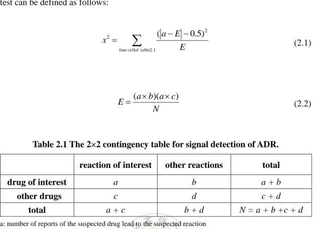
(16) Chapter 2 Background and Related Work 2.1 ADR Detection As we have mentioned in Section 1.1, the main purpose of spontaneous reporting systems is to collect as could as possible all adverse drug events to facilitate the detection of suspected ADR signals via some statistical or data mining methods. Contemporary detection methods of ADR signals can be broadly divided into two categories: frequentist methods and Bayesian methods [6]. In the following of this chapter, we will describe representative methods and measurements of each category.. 2.1.1 Frequentist methods Frequentist methods are widely used in most real ADR monitoring systems due to their simplicity to calculate and interpret. This category is mainly based on the statistical 2*2 contingency table as shown in Table 2.1 to estimate the proportion of suspected ADRs in spontaneous reporting systems caused by the drug of interest vs. other drugs. If the ratio is higher than a threshold, then disproportionality occurs, which means the drug of interest is regarded to have a significant association with the suspected reaction. In the past decade, there have been various frequentist methods, each of which differs mainly on the metric for measuring the disproportionality [10]. The most representative metrics are Proportional Reporting Ratio (PRR) and Reporting Odds Ratio (ROR) [20]. In addition, hypothesis tests of independence, i.e., chi-square test, are usually adopted as extra precautionary measures. The formula of chi-square 5.

(17) test can be defined as follows:. ( a  E  0.5)2. . x2 . E. (2.1). E. four cellof table2.1. (a  b)(a  c) N. (2.2). Table 2.1 The 2×2 contingency table for signal detection of ADR. reaction of interest. other reactions. total. drug of interest. a. b. a+b. other drugs. c. d. c+d. total. a+c. b+d. N = a + b +c + d. a: number of reports of the suspected drug lead to the suspected reaction b: number of reports of the suspected drug lead to all other reactions c: number of reports of all other drugs in the database lead to the suspected reactions d: number of reports of all other drugs lead to all other reactions.. The PRR measure proposed by Evans et al. [11] is used by UK medicines and Healthcare products Regulatory Agency (MHRA) [11]. PRR is defined as the ratio of ADR reports for the suspected drug that are related to a specific adverse reaction, divided by the corresponding ratio for all other drugs in the database, which is defined as follows: PRR . a /( a  b) c /( c  d ). (2.3). The ROR measure is used by the Netherlands Pharmacovigilance Centre Lareb [9]. ROR is defined as the proportion of a specific ADR caused by the suspected drug to all other drugs in the database, divided by the corresponding proportion of other adverse reactions, which is defined as follows: 6.

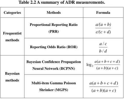
(18) ROR . a/c b/d. (2.4). 2.1.2 Bayesian methods Another category of more complex methods, Bayesian methods were developed based on Bayesian statistics to estimate the (posterior) probability that the suspected adverse reaction occurs given the use of the suspected drug. Representatives of this category are Bayesian Confidence Propagation Neural Network (BCPNN) [2][3][17] and Multi-item Gamma Poisson Shrinker (MGPS) [1]. The Bayesian confidence propagation neural network (BCPNN) is used by WHO Uppsala Monitoring Centre (UMC), while the Multi-item Gamma Poisson Shrinker (MGPS) is applied by US Food and Drug Administration (FDA). BCPNN is mainly to calculate an information component (IC) value. The IC value measures the strength of association between a drug and an adverse reaction. The IC measure is defined in the following:. IC  log 2. p ( x, y ) p( x) p( y ). can be estimated by log 2. a(a  b  c  d ) ( a  b)(a  c). (2.5). where p (x) is the probability of the drug x appears in the reports, p ( y ) is the probability of the reaction y appears in the reports, and p( x, y ) is the probability of both drug x and reaction y appear in the reports. Since the distribution of IC is difficult to determine, instead usually the beta distribution is assigned a prior to the following four probabilities in computing IC.. p( x) ~ B(1 ,  2 ) , p( y ) ~ B( 1 ,  2 ) , p( x, y ) ~ B(1 ,  2 ). 7. (2.6).

(19) The computation is very complicated and beyond our discussion. The readers can refer to [14] for more detailed derivation. MGPS concludes the strength of association between the suspected drug and the suspected reaction by estimating the number of reports containing both the suspected drug and the suspected reaction in database and the expected value. This measure, called relative rate (RR) [29], is defined from the definition of probabilistic independence, defined in the following:. RR . p( x, y ) a(a  b  c  d )  p( x) p( y ) (a  b)(a  c). (2.7). In the field of adverse drug reactions, most of detection methods can be used and every method has its own advantages and disadvantages. Therefore, one can select one or more suitable detection methods according to different analysis purposes. A summary of the mentioned ADR measures are shown in Table 2.2. Table 2.3 summarizes the most frequently used signal detection methods.. Table 2.2 A summary of ADR measurements. Categories. Frequentist. Methods. Formula. Proportional Reporting Ratio. a/(a  b). (PRR). c/(c  d). methods. a/c. Reporting Odds Ratio (ROR). b/d Bayesian Confidence Propagation Neural Network (BCPNN). log 2. a(a  b  c  d ) ( a  b)(a  c). Bayesian methods. Multi-item Gamma Poisson. a(a  b  c  d ). Shrinker (MGPS). ( a  b)(a  c ). 8.

(20) Table 2.3 A summary of signal detection methods for identifying ADRs. Categories. Methods. Threshold. Application. Reference. U.K. Yellow Card. [11],[25],. database. [26]. 95% CI  1. 95%CI  e Proportional. ln( PRR) 1.96 SE. 1 1 1 1    a a b c c  d. SE . Reporting UK Medicines and. Ratio (PRR). 2. PRR  2, x  4, a  3. Frequentist. Healthcare products [9] Regulatory Agency (MHRA). methods [9]. PRR >1. 95% CI  1 Reporting. 95%CI  e. ln( ROR) 1.96 SE. [9],[25], Pharmacovigilance [26]. Odds Ratio (ROR). Netherlands. SE . 1 1 1 1    a b c d. Centre Lareb. ROR > 1. [9]. Bayesian Confidence WHO Uppsala. Propagation Neural. IC  2 SD  0. [2],[3]. (UMC). network Bayesian. Monitoring Centre. (BCPNN). methods Multi-item US Food and Drug. Gamma Poisson. EB05  2, a  3. Administration (FDA). Shrinker (MGPS). 9. [1].

(21) 2.2 Rough Set Theory The rough set theory originally proposed by Z. Pawlak in 1982 [24] is a useful tool for the analysis of imprecise, uncertainly or incomplete data. The theory is based on the concept of rough set, a formal approximation of a crisp set composed of objects represented by values of attributes. Classically, the set of objects concerned is represented as an information system or information table [28]. In the following, we introduce the basic concepts of rough sets theory and use rough set theory to data with missing values.. 2.2.1 Basic Concepts Information System An information system is a pair S  {U , A} [33], where U denotes a nonempty finite set of objects called the universe and A denotes a nonempty finite set of attributes. For example, a data set contains the basic information for students in Table 2.4. This data set can use terminology of the rough set theory as an information system, where universe U represents the set of cases U  {1,2,3,4} and A represents the set of variables i.e., A  {Height , Weight , Gender} . Table 2.4 An example of information system. Case. Height. Weight. Gender. 1. 170. 60. Male. 2. 165. 55. Female. 3. 155. 45. Female. 4. 150. 65. Male. 10.

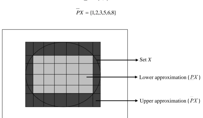
(22) Decision Table (Data Table) A decision table is a special form of information systems, in which the set attribute A is divided into a set of conditional attributes C and a decision attribute d, i.e.. A  C  {d } . For example, in Table 2.5 there are three condition attributes A  {Height , Weight , Age} , and one decision attribute d  {Overweight} .. Table 2.5 An example of decision table. Case. Height. Weight. Age. Overweight. 1. 170. 75. 18. Yes. 2. 165. 50. 30. Yes. 3. 165. 60. 18. No. 4. 145. 75. 18. No. 5. 145. 50. 30. No. 6. 170. 45. 45. Yes. 7. 145. 50. 45. No. 8. 170. 45. 30. Yes. Lower and Upper Approximations The following definition defines two basic concepts for applying rough set theory to data analysis: the lower and upper approximations. Let X represent a subset of elements of the universe U. The lower approximation indicates the set of elements certainly belonging to the set X, while the upper approximation indicates the set of elements possibly belonging to the set X. Given an information system S  (U , A) and. P  A , the lower approximation of X induced by P in S, denoted as P X , and the upper approximation of X induced by P in S, denoted as P X , are defined as follows: 11.

(23) PX  {e U | [e]  X } P. PX  {e U | [e]  X  } P. where [e]P denotes the equivalence class of e induced by attribute set P. Figure 2.1 is a conceptual illustration of the lower and upper approximations of a subset X in U induced by P. For example, let X = {1, 2, 6, 8} and P = {Weight, Age}, then the lower and upper approximations of X induced by P are:. PX  {6,8}. PX  {1,2,3,5,6,8}. Set X Lower approximation (. ). Upper approximation (. ). Figure 2.1 Illustration of the lower and upper approximations of rough set theory.. Accuracy of Approximations The accuracy of an approximation of X induced by P, denoted as  P ( X ) , is calculated as dividing the cardinality of the lower approximation by the cardinality of the upper approximation, 12.

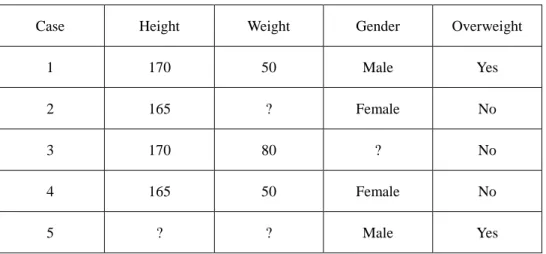
(24) P ( X ) . PX PX. If  P ( X )  1 , the lower and upper approximations are identical, which indicates the set X is definable in U. If  P ( X )  1 , set X can be defined by its lower and upper approximation and is roughly definable in U. For example, from Table 2.5 we can obtain the accuracy of approximations in the following:. P ( X ) . 2 1  6 3. 2.2.2 Rough Set Strategies to Data with Missing Data In real world applications, any data collections usually contain missing values, making the data incomplete for analysis. Various researchers have extended rough set theory for dealing with data with missing values [13][19][31]. In this section, we present the concepts that are useful in our research, mainly the characteristic relation, characteristic set, and the refined lower and upper approximations. Classically, the data is usually presented in the form of a decision table, where missing values can be interpreted from two aspects: lost and do not care. A lost missing value, denoted as “?”, indicates that the value is important but is erased (see Table 2.6). A don’t care missing value, denoted as “*”, indicates that the value is not important or redundant (see Table 2.7). In Table 2.8, we present a decision table with missing values of both categories: lost and don’t care.. 13.

(25) Table 2.6 An example of an incomplete decision table containing “lost” missing values. Case. Height. Weight. Gender. Overweight. 1. 170. 50. Male. Yes. 2. 165. ?. Female. No. 3. 170. 80. ?. No. 4. 165. 50. Female. No. 5. ?. ?. Male. Yes. Table 2.7 An example of an incomplete decision table containing “don’t care” missing values. Case. Height. Weight. Case. Overweight. 1. 170. 50. Male. Yes. 2. 165. *. Female. No. 3. 170. 80. *. No. 4. 165. 50. Female. No. 5. *. *. Male. Yes. Table 2.8 An example of an incomplete decision table containing “lost” and “don’t care” missing values. Case. Height. Weight. Case. Overweight. 1. 170. 50. Male. Yes. 2. 165. ?. Female. No. 3. 170. 80. ?. No. 4. 165. 50. Female. No. 5. *. *. Male. Yes. 14.

(26) Characteristic relation & Characteristic set The conventional rough set theory is under the assumption that information systems are complete and relies on the indiscernibility relation to derive other kernel definitions such as lower and upper approximations. However, the indiscernibility relation is not applicable to data with missing values. Different extensions of the indiscernibility relation have been proposed, including the tolerance relation [19], similarity relation [31], and characteristic relation [13]. The tolerance relation was proposed by Kryszkiewicz to process data with “don’t care” missing values, the similarity relation was proposed by Stefanowski and Tsoukias to process data with “lost” missing values, while the characteristic relation, proposed by Grzymala-Busse, considers both “lost” and “don’t care” missing values. Since the characteristic relation is a general form of the tolerance and similarity relations, in this thesis we adopt this term (denoted as R), and use subscripts T and S to denote the tolerance (RT) and similarity versions (RS), respectively.. Definition 2.1 Let P  A be a subset of attributes. The similarity characteristic relation, denoted by RS (P) , is denoted as:. ( x, y )  RS ( P ) if and only if  ( x, a )   ( y , a ) for all a  P such that  ( x, a )  ?.. And the similarity characteristic set K S (x) is defined as: K s ( P, x)  { y | ( x, y )  Rs ( P)}. 15.

(27) Example 2.1 Consider Table 2.6. Let P be the set of all attributes. Then the similarity characteristic sets of all cases induced by P are:. K S ( P,1)  {1} K S ( P,2)  {2,4} K S ( P,3)  {3} K S ( P,4)  {4} K S ( P,5)  {1,5}. Defintion 2.2 Let P  A be a subset of attributes. The tolerance characteristic relations, denoted by RT ( p) , is defined as:. ( x, y )  RT ( P ) if and only if  ( x, a )   ( y , a ) or.  ( x, a )  * or  ( y , a )  * for all a  P .. And the tolerance characteristic set KT ( P, x) is defined as:. KT ( P, x)  { y | ( x, y)  RT ( P)}. where x and y are two cases in the decision table, and  ( x, a) denotes the value of x in attribute a.. Example 2.2 Consider Table 2.7. Let P be the set of all attributes. Then the tolerance characteristic sets of all cases induced by P are:. 16.

(28) KT ( P,1)  {1,5} KT ( P,2)  {2,4} KT ( P,3)  {3,5} KT ( P,4)  {2,4} KT ( P,5)  {1,3,5} Definition 2.3 Let P  A be a subset of attributes. The characteristic relation, denoted by R(P) , is defined as:. ( x, y )  R( P) if and only if  ( x, a )   ( y, a ) or.  ( x, a )  * or  ( y, a )  * for all a  P such that  ( x, a )  ? .. And the characteristic set K ( P, x) is defined as K ( P, x)  { y | ( x, y )  R( P)}. Example 2.3 Consider Table 2.8. Let P be the set of all attributes. Then the characteristic sets of all cases induced by P are: K ( P,1)  {1,5} K ( P,2)  {2,4} K ( P,3)  {3,5} K ( P,4)  {4} K ( P,5)  {1,5}. Based on the concept of characteristic relation and characteristic set, GrzymalaBusse [13] proposed three different extensions of the lower and upper approximations for processing data with missing values: singleton, subset, and concept approximations. The first extension is called singleton approximation, which considers all cases in 17.

(29) U and is similar to the original definitions of lower and upper approximations.. Definition 2.4 The singleton lower approximation of X induced by P, denoted by p gk X , is the set of all cases whose characteristic set is contained in X, i.e.,. P g X  { x U | K P ( x )  X } k. k. The singleton upper approximation of X in P, denoted by P g X , is the set of cases whose characteristic set of having an non-empty intersection with X, i.e.,. k. P g X  {x U | K P ( x )  X   }. Note that the characteristic sets presented in the above definition can be any types of characteristic sets.. Example 2.4 Consider Table 2.6. There are two equivalence classes induced by attribute Overweight, i.e., {1, 5} and {2, 3, 4}. Below are the singleton approximations of these two elementary sets:. P g {1,5}  {1,5} K. P g {2,3,4}  {2,3,4} K. K. P g {1,5}  {1,5} K. P g {2,3,4}  {2,3,4} The second extension, called subset approximation, uses the union of characteristic sets to define approximation.. 18.

(30) K. Definition 2.5 The subset lower approximation of X induced by P, P s X , is the union of characteristic sets that are contained in X, i.e.,. P sK X  {K ( p, x) | x U , K ( p, x)  X }. K. The subset upper approximation of X induced by P, P s X , is the union of characteristic sets which have an nonempty intersection with X, i.e.,. P sK X  {K ( P, x) | x U , K ( P, x)  X  }. Example 2.5 Continuing with Example 2.4, the subset approximations of the two elementary sets induced by Overweight are: P S {1,5}  {1,3,5} k. P S {2,3,4}  {1,2,3,4,5} k. k. P S {1,5}  {1,5} k. P S {2,3,4}  {2,4} The third definition called concept approximation is stricter than the subset version in that it only considers those cases in X.. Definition 2.6 The concept lower and upper approximations of X induced by P are defined as follows:. PcK X  {K ( P, x) | x  X , K ( P, x)  X } K. Pc X  {K ( P, x) | x  X , K ( P, x)  X  }. Example 2.6 Continuing with Example 2.4, the concept approximations of the two elementary sets induced by Overweight are: 19.

(31) P c {1,5}  {1,3,5} K. P c {2,3,4}  {2,3,4,5} K. K. P c {1,5}  {1} K. P c {2,3,4}  {2,4}. Note that for complete decision tables, all of the three approximations, singleton, subset, and concept, are amalgamated into the same definition. However, it is not true for incomplete decision tables.. 2.3 Rough Set in Medical Informatics Application Medical databases usually contain a lot of incomplete or ambiguous data, and for some applications the amount of data is very huge [8]. Therefore, it is natural to develop rough set based intelligent methods for analyzing medical data [4][5][15][27][31]. Representative techniques include rough set based medical image segmentation [21], rough set based medical classifications and pattern recognitions [18][32], and rough set based medical diagnosis [22]. Since the ADR signal detection problem bears a resemblance to medical classification and diagnosis, below we only highlight related work on these topics. Mandal et al. [22] used originally concept of rough set theory for the automated diagnosis of Lung Adenocarcinoma and to predict genes of patients causing the Lung Adenocarcinoma. They used publicly microarray dataset obtained from the NCBI website. Experimental results via cross validation exhibit 100% accuracy for the discovered rules. Hassanien and Ali [16] used rough set method for generating classification rules 20.

(32) from the breast cancer data. They used attribute reduction technique of rough set theory to select the necessary attributes. The purpose is to identify every decision class by using the minimum condition which can increase efficiency for decision making. The generated rules and classification accuracy was compared with decision tree classifier algorithm, which showed that the rough set based approach produces stricter rules and the classification accuracy is higher than that of decision trees. Stepaniuk [30] used rough set theory to identify the most important condition attributes and according to the condition attributes and decision attribute produced decision rules from the diabetes mellitus dataset. The proposed method can be applied to different kinds of medical datasets. The above literatures highlight the usefulness and efficiency of rough set theory in medical domain. In summary, the concept of rough set theory can aid building medical information systems or expert systems in medical domain, and can provide medical experts to analyze the problem effectively.. 21.

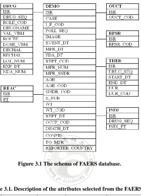
(33) Chapter 3 Rough Set Based ADR Detection 3.1 Problem Description As mentioned in Chapter 1, spontaneous reporting systems are used to monitor and discover suspicious ADR signals. When the patient produces uncomfortable or harmful adverse reaction by normal drug of usage, hospitals, pharmaceutical companies, and the patient himself can report or query by SRS. The reporting data may contain some missing values due to omitting or personal privacy problem. The purpose of this study is to consider records with missing values and use rough set strategies to process the reporting data with missing values. In this study, the reporting data is obtained from the FDA Adverse Event Reporting System (FAERS) database [12]. The FAERS database is composed of seven data files, as shown in Figure 3.1, including DEMO, DRUG, REAC, OUTC, RPSR, THER, and INDI. We selected three data files that are essential for ADR signal detection, i.e., DEMO, DRUG, and REAC. From the DEMO data file, we chosen four attributes about personal information of patients, including ISR (primary report id), EVENT_DT, AGE, and GNDR_COD. These attributes may contain null values except ISR. From the DRUG and REAC files we chosen the DRUGNAME and PT attributes, which do not contain null values. Details of the chosen attributes are presented in Table 3.1. Table 3.2 is a snapshot of the reporting data extracted from data collected in the first quarter of 2008.. 22.

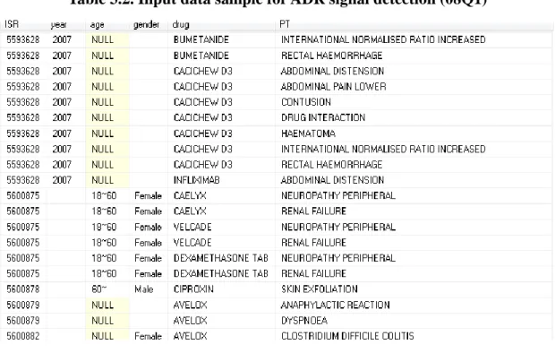
(34) Figure 3.1 The schema of FAERS database.. Table 3.1. Description of the attributes selected from the FAERS dataset Selected. Containing. Null probability. Attribute name. attribute name. null values. (07Q2). descriptions. ISR. . 0. number of patients (unique). EVENT_DT. . 31.3. adverse event happen date. AGE. . 38.8. age of patients. GNDR_COD. . 5.8. gender of patients. DRUG. DRUGNAME. . 0. Name of drug (trade name). PT. . 0. Name of ADR (using PT. REAC. File name. DEMO. level from MedDRA ). DEMO: to record personal information for each patient. DRUG: to record the medicines taken by each patient. REAC: to record the observed adverse reactions for each report. 23.

(35) Table 3.2. Input data sample for ADR signal detection (08Q1). To facilitate the discussion, the reporting data is presented as an information system S  (U , A) containing missing values. Further, we assume that the reporting data is indicated in the form of an incompletely data table, and that the missing values can be either one of two categories: lost (?) or don’t care (*). Our purpose is to examine the feasibility of rough set theory to the ADR detection, focusing on whether the inclusion of missing data through rough set based approximation can be helpful for the predicting capability of generated signals. Therefore, the problem can be described as given a SRS dataset extracted from the FAERS database that contains missing values and is represented in the form of data table, we like to compute the strength (using PRR or ROR measure) of any given suspected ADR rule of the following form: Predc, drug  symptom. (3.1). where Predc denotes extra conditions associated with the signal, e.g., Sex = “female”, Age = “>18” and examine if the strength of this rule is over a specified threshold to becoming a noteworthy ADR signal. 24.

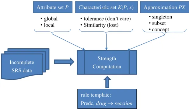
(36) 3.2 Rough Set Based Method: Basic Idea Since all contemporary measures relies on the contingency 22 table, our basic idea is applying rough set theory to the calculation of the contingency 22 table. Consider the rule in (3.1) and the following corresponding contingency table.. Predc. symptom Other symptoms. drug. a. b. Other drugs. c. d. If the information system is complete, then each of the cell values, a, b, c, d, on the contingency table are deterministic. Unfortunately, as we have shown previously, the attributes involved in the Predicate may contain missing values, causing the cell values imprecise. We thus adopt the concept of lower and upper approximations to obtain an approximate range of each cell values and in accordance compute the strength of the corresponding rule. For simplicity, let Xa, Xb, Xc, and Xd denote the sets of cases satisfying the corresponding cell conditions in the contingency table. Clearly, for complete data we have a  |Xa|, b  |Xb|, c  |Xc|, and d  |Xd|. But for incomplete data we compute the lower and upper approximations for Xa, Xb, Xc, and Xd. Let P denote the set of attributes for the approximation computation. Each cell value can be denoted by a range, i.e.,. a: [𝑎̅, 𝑎], b: [𝑏̅, 𝑏], c: [𝑐̅, 𝑐], d: [𝑑̅ , 𝑑],. 25. (3.2).

(37) and accordingly, we have 𝑎̅  |𝑃KXa|, 𝑎  |PKXa|, 𝑏̅  |𝑃KXb|, 𝑏  |PKXb|,. (3.3). 𝑐̅  |𝑃KXc|, 𝑐  |PKXc|, 𝑑̅  |𝑃KXd|, 𝑑  |PKXd|. We consider two different options for defining the set P: global and local. The global approach specifies all attributes in the data to P, i.e., P = A. The local approach instead only considers the set of attributes forming the rule of concern (and so the contingency table). For convenience, we denote this attribute set as B, for B  A. Note that following the definitions in Section 2.2.2, there are two different interpretations of missing values, i.e., lost or don’t care, and three different versions of approximations, i.e., singleton, subset, and concept approximations. In total, there are 12 different ways for computing the cell values defined in (3.2) and (3.3), as shown in Figure 3.2. Figure 3.2 also shows the research framework adopted in this study, inspecting the feasibility for applying rough set theory to the ADR signals detection from an incomplete SRS dataset containing missing values. We assume that the template of the rule to be discovered is given, either by the user or generated by a pre-procedure of candidate rule generation. In the reminder of this chapter, we will examine the feasibility of the 12 ways (versions) for computing the cell values in Section 3.3 and then describe the algorithmic details for completing the work in Section 3.4.. 26.

(38) Attribute set P • global • local. Characteristic set K(P, x) • tolerance (don’t care) • Similarity (lost). Approximation PX • singleton • subset • concept. Strength Computation. Incomplete SRS data. rule template: Predc, drug  reaction Figure 3.2 The research framework for incomplete ADR signal detection. 3.3 Feasibility Analysis In this section, we analyze the feasibility of the 12 different methods presented in Section 3.2, examining whether each one of them can appropriately yield reasonable approximations for data with missing values. To facilitate the discussion, we first introduce the concept of satisfiable approximation and indistinguishable approximation. Consider a rule of the form defined in (3.1) and the corresponding contingency table. Let C be the attribute set for defining the extra conditions Predc for forming the contingency table.. Definition 3.1 Let y be any case in U. We say y satisfies the Predc condition if for each attribute t in C, (y, t)  (Pred, t) or (y, t)  ? or (y, t)  *, where (Pred, t) denotes the condition value of attribute t in Predc.. 27.

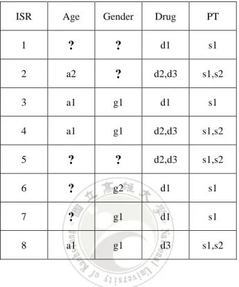
(39) Note that in the above definition we adopt the concepts used by tolerance or similarity relation to maintain the compatible. That is, we omit the attributes with missing values when inspecting the condition.. Definition 3.2 An approximation of the contingency sets X (X can be either Xa, Xb, Xc, or Xd) defined on an attribute set P is a C-satisfiable approximation if all members in either the lower approximation PX or upper approximation P X satisfy the Predc conditions specified by C.. Example 3.1 Consider the data table with lost missing values in Table 3.3. We would like to compute the strength of the following rule: Gender  g2, Drug  d2  PT  s1 The corresponding contingency table for this purpose is shown in Table 3.4, where Xa  {4}, Xb  , Xc  {3, 7, 8}, and Xd  , and C = {Gender}. Now assume the subset approximation with similarity characteristic set and global covering is applied. Then, we can obtain the following characteristic sets of all cases in Table 3.3. K S ( P,1)  {1,3,6,7}. K S ( P,5)  {2,4,5}. K S ( P,2)  {2}. K S ( P,6)  {6}. K S ( P,3)  {3}. K S ( P,7)  {3,7}. K S ( P,4)  {4}. K S ( P,8)  {8}. Below are the lower and upper approximations of Xa, Xb, Xc, and Xd. P X a  {4}. P X a  {4}. PX b  . PX b  . P X c  {3,7,8}. P X c  {1,3,6,7,8}. PX d  . PX d   28.

(40) Note that case 6 in the upper approximation of Xc contradicts the condition Gender  g2. Therefore, the subset approximation with similarity characteristic set and global covering is not C-satisfiable.. Table 3.3 An incompletely data table with lost missing values. ISR. Age. Gender. Drug. PT. 1. ?. ?. d1. s1. 2. a2. ?. d2,d3. s1,s2. 3. a1. g1. d1. s1. 4. a1. g1. d2,d3. s1,s2. 5. ?. ?. d2,d3. s1,s2. 6. ?. g2. d1. s1. 7. ?. g1. d1. s1. 8. a1. g1. d3. s1,s2. Definition 3.3 An approximation of the contingency sets X (X can be anyone of Xa, Xb, Xc, and Xd) defined on an attribute set P, PX (PX), is an indistinguishable approximation if the lower approximation of the contingency set X is always equal to the corresponding upper approximation, i.e., PX = PX.. Table 3.4 The contingency table corresponding to the four contingency sets described in Example 3.1. Gender = g1. PT = s1. other PT. Drug = d2. {4}. {}. other drugs. {3,7, 8}. {}. 29.

(41) Example 3.2 Consider Table 3.3 and the rule in Example 3.1 again. Assume that the concept approximation with similarity characteristic set and global covering is applied. Below are the lower and upper approximations of Xa, Xb, Xc, and Xd.. P X a  {4}. P X a  {4}. PX b  . PX b  . P X c  {3,7,8}. P X c  {3,7,8}. PX d  . PX d  . Since the lower and upper approximations are the same, this approximation is indistinguishable. Lemma 3.1 The subset approximation defined by tolerance characteristic set KT for contingency sets Xa, Xb, Xc, and Xd, is not C-satisfiable with respect to P, for P  B. Proof. We only consider the case of Xa and P  B. It is easy to apply similar strategies to prove other cases. To prove PKs T Xa is not C-satisfiable, we will show that indeed, the KT. upper approximation Ps Xa is not C-satisfiable. KT. Consider a member y in Ps Xa. And we assume that y belongs to the tolerance characteristic set of some case x induced by P, i.e., y  KT(P, x). According to the KT. definition of Ps X, we know KT(P, x) ∩ Xa  , which implies that it is possible that y  Xa. The lemma then follows. ∎. Lemma 3.2 The subset approximation defined by similarity characteristic set KS for contingency sets Xa, Xb, Xc, and Xd, is not C-satisfiable with respect to P, for P  B. Proof. The proof is similar to that in Lemma 3.1. ∎. 30.

(42) Lemma 3.3 The concept approximation defined by similarity characteristic set KS is indistinguishable for contingency sets Xa, Xb, Xc, and Xd, with respect to P, for P  B, KS. i.e., PKc S X = Pc X, for X being any of Xa, Xb, Xc, or Xd. Proof. Again, we only consider the case of Xa and P  B. Recall the following KS. definitions for PKc S Xa and Pc Xa.. PKc S Xa ∪{KS(P, x)| x  Xa, KS(P, x)  Xa} KS. Pc Xa ∪{KS(P, x)| x  Xa, KS(P, x) ∩ Xa  }. According to the definition of KS(P, x), if a case y  KS(P, x), then (x, t)  (y, t) for all attribute t  P and (x, t)  ?. Since x  Xa, it follows that all attribute values of x in B are not lost, i.e., for all t  B, (x, t)  ?, and so are y. This means if y  KS(P, x) then y  Xa as well. In other words, KS(P, x)  Xa and we have KS. PKc S Xa  Pc Xa Xa, which proves the lemma. ∎. It is interesting to note that in the proof of Lemma 3.3, if the concept approximation is defined by the tolerance characteristic set, then a member y  KS(P, x) may not belong to Xa. This is because y may contain some don’t care attributes in B, which hinders it from a member of Xa. Although we do not discuss, in terms of the satisfiable and ineffective concept, it is not hard to show all the other approximations defined in Section 3.2 are C-satisfiable 31.

(43) and effective. In summary, the 12 approximation methods can be divided into two categories, the feasible methods and the unfeasible methods, by examining whether they are satisfiable and indistinguishable or not, i.e., (1) Unsatisfiable: The results of the lower and/or upper approximations include some infeasible case that contradicts to the predicate conditions specified for the rule of concern. (2) The lower and upper approximations produce the same results. Table 3.5 summarizes the two groups of feasible and infeasible approximation methods. We obtain six feasible approximation methods for computing the four contingency sets. For convenience, we denote the six methods in terms of the characteristic sets (similarity or tolerance), attribute covering (global or local), and approximation definitions (singleton, subset, or concept), as follows: Method 1 M(s, g, g): Similarity set, global covering, singleton approximation Method 2 M(s, l, g): Similarity set, local covering, singleton approximation Method 3 M(t, g, g): Tolerance set, global covering, singleton approximation Method 4 M(t, l, g): Tolerance set, local covering, singleton approximation Method 5 M(t, g, c): Tolerance set, global covering, concept approximation Method 6 M(t, l, c): Tolerance set, local covering, concept approximation. 32.

(44) Table 3.5 Summarization of the feasible and infeasible approximation methods. Lost. Don’t care. (Similarity characteristic set). (Tolerance characteristic set). Global. Local. Global. Local. Singleton. . . . . Subset. . . . . Concept. x. x. . . : feasible approximation : infeasible approximation, due to unsatisfiable property x: infeasible approximation, due to indistinguishable property. 3.4 The Detection Method In this section, based on the presented approximation for measuring the contingency values we will describe our ADR detection algorithm. First in subsection 3.4.1, we present our method in a general algorithmic framework, and then demonstrate the algorithm with a simple example in subsection 3.4.2.. 3.4.1 Algorithm Description Given a SRS dataset with missing values, we assume that the rule representing the ADR signal to be discovered is provided by the user. Our algorithm, as shown in Figure 3.3, computes the strength of the rule according to the following parameters, attribute covering (global or local), characteristic set (tolerance or similarity), approximation (singleton, subset, or concept), and the signal measure (PRR or ROR).. 33.

(45) Input: . STab: the SRS data table;. . RTemp: the rule template;. . ACtype: the type of attribute coverings;. . CStype: the type of characteristic sets;. . APtype: the type of approximations;. . MStype: the type of measures.. Output: The rule and the strength. Steps: 1.. Compute the characteristic sets of all records in STab according to ACtype and CStype;. 2.. Generate the four contingency sets, Xa, Xb, Xc, and Xd, according to the rule template RTemp;. 3.. Generate the lower and upper approximations of Xa, Xb, Xc, and Xd, according to the choosed approximation APtype;. 4.. Compute the rule strength using the approximate contingency X*a, X*b, X*c, and X*d, according to the measure MStype;. 5.. Return the rule with the computed strength; Figure 3.3 Algorithmic framework of the proposed ADR detection method The execution process is divided into four main phases: (1) Compute the characteristic sets of each case in SRS; (2) Generate the initial four contingencey sets, Xa, Xb, Xc, and Xd; (3) Generate the lower and upper approximations of Xa, Xb, Xc, and Xd; (4) Computing the strength of the rule in PRR or ROR measure; In the following, we will describe each of the phases.. 34.

(46) Phase 1: Compute the characteristic sets The main task of this phase is, considering the missing values, to find similar cases of each case in the input data table. According to the definition of similarity characteristic set, if the missing values are indicated by lost (?), the process compares all attribute fields of two cases except those attribute values being null. On the other hand, if the missing values are indicated by don’t care (*), the process compares the specific attribute fields of two cases, and the null values are regarded as all possible values for the corresponding attribute field. The algorithm responsible for this phase is described in Figure 3.4.. Input: The data table STab, attribute covering type ACtype, characteristic set type CStype. Output: The characteristic sets of all cases, denoted by KS; Steps: 1. 2. 3.. for each case r1  ST do for each case r2  ST and r1  r2 do if ACtype = ‘global’. 4.. then attribute set P  A;. 5.. else P  B;. 6.. // B denotes the set of attributes in RTemp;. if CStype = ‘similarity’ then if (for all fields f  P, r1.f  r2.f or r1.f  null). 7. 8.. store r2 into KS(r1);. 9.. else if CStype = ‘tolerance’ then if (for all fields f  P, r1.f  r2.f or r1.f  null or r2.f  null). 10. 11. 12. 13.. // r2 is a similar case to r1;. store r2 into KS(r1);. // r2 is a similar case to r1;. endif endfor Figure 3.4 Algorithm for computing characteristic set. 35.

(47) Phase 2: Generate the contingency sets The purpose of this phase is to obtain the initial four contingency sets Xa, Xb, Xc, and Xd, which correspond to the cells in the contingency table used for evaluating the strength of the rule. This phase is easy to be implemented, by simply inspecting each case in the data table ST against the corresponding conditions implicitly specified by the rule template RTemp, and assign the case into the corresponding contingency set. Note that all cases with missing values appear in the attributes composed of the rule are ignored in this phase. We omit the algorithmic description of this procedure due to its simplicity.. Phase 3: Compute the lower and upper approximations After the characteristic sets of all cases and the four contingency sets are ready for use, then we can proceed to this phase, which is, according to the type of approximation operation APtype, responsible for computing the lower and upper approximations for the four contingency sets, which are denoted as X*a, X*b, X*c, and X*d. For clarity, we separate this phase into two procedures, one for lower approximation (see Figure 3.5), and the other for upper approximation (see Figure 3.6).. Phase 4: Calculate the rule strength The final phase is to calculate the measure value of the rule, either in PRR or ROR. First, we count the approximate contingency values, a*, b*, c*, and d*, simply corresponding to the cardinalities of their lower and upper approximate contingency sets, i.e., a* = [| Xa |, | X a |], b* = [| Xb |, | X b |], c* = [| Xc |, | X c |], d* = [| Xd |, | X d |].. 36.

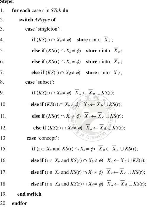
(48) Input: The characteristic set KS, the contingency sets Xa, Xb, Xc, and Xd, and the approximation type APtype. Output: The lower approximations of Xa, Xb, Xc, and Xd, denoted by Xa, Xb, Xc, and Xd. Steps: 1. 2. 3.. for each case r in STab do switch APtype of case ‘singleton’:. 4.. if (KS(r)  Xa) store r into Xa;. 5.. else if (KS(r)  Xb) store r into Xb;. 6.. else if (KS(r)  Xc) store r into Xc;. 7.. else if (KS(r)  Xd) store r into Xd;. 8.. case ‘subset’:. 9.. if (KS(r)  Xa) Xa  Xa ∪KS(r);. 10.. else if (KS(r)  Xb) Xb  Xb ∪KS(r);. 11.. else if (KS(r)  Xc) Xc  Xc ∪KS(r);. 12.. else if (KS(r)  Xd) Xd  Xd ∪KS(r);. 13.. case ‘concept’:. 15.. if (r  Xa and KS(r)  Xa) Xa  Xa ∪KS(r);. 16.. else if (r  Xb and KS(r)  Xb) Xb  Xb ∪KS(r);. 17.. else if (r  Xc and KS(r)  Xc) Xc  Xc ∪KS(r);. 18.. else if (r  Xd and KS(r)  Xd) Xd  Xd ∪KS(r);. 19.. end switch. 20. endfor Figure 3.5. Algorithm for computing lower approximations.. 37.

(49) Input: The characteristic set KS, the contingency sets Xa, Xb, Xc, and Xd, and the approximation type APtype. Output: The upper approximations of Xa, Xb, Xc, and Xd, denoted by X a , X b , X c , and X d . Steps: 1. 2. 3.. for each case r in STab do switch APtype of case ‘singleton’:. 4.. if (KS(r)  Xa  ). 5.. else if (KS(r)  Xb  ) store r into X b ;. 6.. else if (KS(r)  Xc  ) store r into X c ;. 7.. else if (KS(r)  Xd  ). 8.. store r into X a ;. store r into X d ;. case ‘subset’:. 9.. if (KS(r)  Xa  ) X a  X a ∪KS(r);. 10.. else if (KS(r)  Xb  ) X b  X b ∪KS(r);. 11.. else if (KS(r)  Xc  ) X c  X c ∪KS(r);. 12.. else if (KS(r)  Xd  ) X d  X d ∪KS(r);. 13.. case ‘concept’:. 15.. if (r  Xa and KS(r)  Xa  ) X a  X a ∪KS(r);. 16.. else if (r  Xb and KS(r)  Xb  ) X b  X b ∪KS(r);. 17.. else if (r  Xc and KS(r)  Xc  ) X c  X c ∪KS(r);. 18.. else if (r  Xd and KS(r)  Xd  ) X d  X d ∪KS(r);. 19.. end switch. 20. endfor Figure 3.6. Algorithm for computing upper approximations.. 38.

(50) Then we compute the strength (range value) of the rule by performing a simple range calculation according to the formula of PRR and ROR. The resulting formulas for range PRR and ROR are as follows:. a (c  d ) a (c  d )  PRR  c (a  b ) c ( a  b). (3.4). ad a d  ROR  c b cb. (3.5). 3.4.2 An Example In this subsection, we use the example data in Table 3.6 to illustrate the execution of our algorithm. We assume that the following rule is to be discovered. Gender  g2, Drug  d2  PT  s1 We only demonstrate the case of Method 1, i.e., similarity characteristic set, global covering, and singleton approximation.. Phase 1: Compute the characteristic sets From Table 3.6, we obtain the following characteristic sets for each case. K S ( P,1)  {1,3,6,7} K S ( P,2)  {2} K S ( P,3)  {3} K S ( P,4)  {4} K S ( P,5)  {2,4,5} K S ( P,6)  {6} K S ( P,7)  {3,7} K S ( P,8)  {8} 39.

(51) Table 3.6 An example of incomplete data with all missing values of lost. Case. Attribute. ISR. Year. Age. Gender. Drug. PT. 1. ?. a2. ?. d1. s1. 2. y2. ?. g1. d2,d3. s1,s2. 3. y2. a2. g2. d1. s1. 4. y2. a1. g2. d2,d3. s1,s2. 5. y2. ?. ?. d2,d3. s1,s2. 6. y1. a2. g1. d1. s1. 7. ?. a2. g2. d1. s1. 8. y1. a1. g2. d3. s1,s2. Phase 2: Generate the contingency sets According to the rule of concern, we can obtain the contingency sets shown in Table 3.7.. Table 3.7 The contingency sets after executing Phase 2 over data in Table 3.6. Gender=g2. PT = s1. other reactions. Drug = d2. {4}. {}. other drugs. {3,7,8}. {}. Phase 3: Compute the lower and upper approximations After performing the algorithms described in Figures 3.5 and 3.6, we can obtain the lower and upper approximations for the contingency sets in Table 3.7.. 40.

(52) P{4}  {4}. P{4}  {4,5}. P{}  . P{}  . P{3,7,8}  {3,7,8}. P{3,7,8}  {1,3,7,8}. P{}  . P{}  . Phase 4: Calculate the rule strength First, we obtain the following contingency table.. Gender = g2. PT = s1. other reactions. Drug = d2. [1, 2]. 0. other drugs. [3, 4]. 0. Then the resulting PRR and ROR of this rule are:. 1(3  0) 2(4  0)  0.375  PRR   2.667 4(2  0) 3(1  0). 1* 0 2*0  ROR  4*0 3* 0. Note that the signal strength is unable to be measured by using ROR. If the threshold is set to PRR > 1, then the strength of this rule is very likely to exceed the threshold since the range covers value 1. Therefore, this rule can output as a suspected ADR signal with measurement quality of 0.375/2.667 = 0.14.. 41.

(53) Chapter 4 Experiments 4.1 Experiment Design We conducted a series of experiments to evaluate the effectiveness for our methods. Our proposed six rough set based ADR measuring methods were compared with traditional method with missing data deletion on timeline warning of serious ADR signals. We considered two different missing data deletions, listwise deletion and pairwise deletion. In the former method, an entire record is deleted if any single value is missing, while in the latter method, a record is excluded from analysis only when missing values occur to the attributes under analysis. We used the 2004 to 2013Q3 of FAERS data to do our experiments, and there are about 60,000 to 190000 reports in each quarterly collection. Two groups of drugs were used in these experiments, including withdrawn drugs and non-withdrawn drugs but labeled in the FDA warning list (MedWatch) [23]. All programs were coded in C# and executed on a PC running with Microsoft SQL server 2008 R2. All signals were measured by two criteria, PRR and ROR. The threshold for an ADR rule being significant followed the widely adopted setting, PRR  2 (or ROR. . 2) and a  3 [9], where a denotes the number of reports satisfy the rule. The first experiment considered those drugs withdrawn from the market in the US. The source of information for these drugs can be found in [7] and FDA [12]. We only selected those drugs exhibits known ADRs for specific populations. Table 4.1 lists the detail information for those drugs and the associated ARDs. Since most of them contain not enough cases in the FAERS dataset (yearly number of reports > 3) for conducting meaningful statistics analysis, we finally only obtained three drugs, AVANDIA 42.

(54) TYSABRI, and ZELNORM, as shown in Table 4.2. Analogous to the first experiment, the second experiment considered the known ADRs associated with non-withdrawn drugs. Detailed information can be found in the FDA Safety Information and Adverse Event Reporting Program, called MedWatch [23]. For the same reasons, we finally selected two drugs, WARFARIN and REVATIO, as shown in Table 4.3. For convenience, each ADR in Tables 4.2 and 4.3 is denoted by a rule.. Table 4.1 Drug withdrawn from the market for safety reasons in the US The suitable of. Year Marked. Drug Name. Symptom. group. withdrawn year in US in US. (Age or Gender). XIGRIS. DRUG INEFFECTIVE. 18~. 2001. 2011. 18~. 1999. 2010. 60~. 2000. 2010. 16~. 1997. 2010. 18~. 2003. 2009. Female. 2002. 2007. 5~. 2004. 2005. 18~. 2004. 2005. MYOCARDIAL INFARCTION AVANDIA. DEATH CEREBROVASCULAR ACCIDENT. MYLOTARG. DRUG INEFFECTIVE CEREBROVASCULAR. MERIDIA. ACCIDENT PROGRESSIVE. RAPTIVA. MULTIFOCAL LEUKOENCEPHALOPATHY CEREBROVASCULAR. ZELNORM ACCIDENT NEUTROSPEC. RESPIRATORY DISTRESS PROGRESSIVE. TYSABRI. MULTIFOCAL LEUKOENCEPHALOPATHY. 43.

(55) Table 4.2 Selected withdrawn drugs used in our experiments. The suitable Year No. Drug Name. of group. Marked. (Age or. year in US. Symptom. withdrawn. Rule. in US Gender). MYOCARDIAL R1-1 INFARCTION R1-2. AVANDIA. DEATH. 18~. 1990. 2010. 18~. 2004. 2005. Female. 2002. 2007. CEREBROVASCULAR. R1-3. ACCIDENT R2. PROGRESSIVE TYSABRI. MULTIFOCAL LEUKOENCEPHALOPATHY. R3. CEREBROVASCULAR ZELNORM ACCIDENT. Table 4.3 Selected non-withdrawn drugs used in our experiments. The suitable No. rule. Drug Name. Symptom. Marked. Warning. year in US. year in US. 60~. 1940. 2014/5/13. ~18. 2008. 2014/4/9. of group (Age). MYOCARDIAL R4. WARFARIN INFARCTION. R5. REVATIO. DEATH. 4.2 Evaluation on Withdrawn Drugs 4.2.1 Comparison of rough set based methods We first compared the accuracy of the six rough set based methods. For this purpose, we computed for each method the average accuracy of each rule’s strength over all different quarters, and then obtained the final average over all rules. The 44.

(56) accuracy of rule strength is defined as PRRl / PRRu, where PRRl and PRRu denote the lower and upper PRR values of the rule, respectively. Table 4.4 summarizes the results for PRR; the results for ROR are very similar to those for PRR, and hence are omitted here. Obviously, Method 1 outperforms all the others, while Methods 4 and 6 exhibit the worst performance. Besides, Methods 4 and 6 exhibit identical accuracy for all rules, implying both may exactly the same, which however, requires further investigation. We also depict the value ranges of all rule strength quarterly, both in PRR and ROR measures. The results are displayed in Figures 4.1 to 4.5. It is clearly that Method 1 demonstrates the strictest strength range in all cases, then Method 2, Method 5, and finally Methods 4 and 6. This is comparable to that shown in Table 4.4.. Table 4.4. Accuracy of the six rough set based ADR measurings for withdrawn drugs. Method M1. M2. M3. M4. M5. M6. R1-1. 0.925632. 0.893919. 0.854776. 0.817942. 0.855185. 0.817942. R1-2. 0.909215. 0.880533. 0.851474. 0.822267. 0.852308. 0.822267. R1-3. 0.95911. 0.946946. 0.90303. 0.88489. 0.903306. 0.88489. R2. 0.945024. 0.940282. 0.900471. 0.885366. 0.900471. 0.885366. R3. 0.999676. 0.994358. 0.996117. 0.99404. 0.996117. 0.99404. Total average. 0.947731. 0.931208. 0.901174. 0.880901. 0.901478. 0.880901. No. Rule. 45.

(57) RST ROR_Upper 255. ROR lower of R1-1 for each methods. Marketed year : 1990 Warning year : 2007 Year withdrawn: 2010. (b) RST PRR_Upper 165. 12Q3. 12Q1. 11Q3. 11Q1. 10Q3. 10Q1. 09Q3. 09Q1. 08Q3. 08Q1. 07Q3. 07Q1. 06Q3. 06Q1. 05Q3. 05Q1. 04Q3. 04Q1. 13Q3. 13Q1. 12Q3. 12Q1. 11Q3. 11Q1. 10Q3. 10Q1. 0 09Q3. 0 09Q1. 33. 08Q3. 9. 08Q1. 66. 07Q3. 18. 07Q1. 99. 06Q3. PRR upper of R1-1 for each methods. Marketed year : 1990 Warning year : 2007 Year withdrawn: 2010. 27. 06Q1. 13Q3. M6*-ROR_upper. 13Q1. M5*-ROR_upper. 13Q3. 12Q3. M6*-ROR_lower. 13Q1. 12Q1. 11Q3. 11Q1. M4*-ROR_upper. M5*-ROR_lower. 132. 05Q3. 10Q3. M2*-ROR_upper. M3*-ROR_upper. PRR lower of R1-1 for each methods. 05Q1. 10Q1. M1*-ROR_upper. M4*-ROR_lower. 36. 04Q3. 09Q3. M2*-ROR_lower. M3*-ROR_lower. Marketed year : 1990 Warning year : 2007 Year withdrawn: 2010. 04Q1. 09Q1. M1*-ROR_lower. (a) RST PRR_Lower 45. 08Q3. 08Q1. 07Q3. 07Q1. 06Q3. 06Q1. 05Q3. 05Q1. 04Q1. 13Q3. 13Q1. 12Q3. 12Q1. 11Q3. 11Q1. 10Q3. 10Q1. 09Q3. 09Q1. 0 08Q3. 0 08Q1. 51. 07Q3. 23. 07Q1. 102. 06Q3. 46. 06Q1. 153. 05Q3. 69. 05Q1. 204. 04Q3. 92. 04Q1. ROR upper of R1-1 for each methods. Marketed year : 1990 Warning year : 2007 Year withdrawn: 2010. 04Q3. RST ROR_Lower 115. M1*-PRR_lower. M2*-PRR_lower. M1*-PRR_upper. M2*-PRR_upper. M3*-PRR_lower. M4*-PRR_lower. M3*-PRR_upper. M4*-PRR_upper. M5*-PRR_lower. M6*-PRR_lower. M5*-PRR_upper. M6*-PRR_upper. (c). (d). Figure 4.1 The result of the ROR & PRR lower and upper for R1-1.. 46.

(58) RST ROR_Upper 25. ROR lower of R1-2 for each methods. (b) RST PRR_Upper 25. 12Q3. 12Q1. 11Q3. 11Q1. 10Q3. 10Q1. 09Q3. 09Q1. 08Q3. 08Q1. 07Q3. 07Q1. 06Q3. 06Q1. 05Q3. 05Q1. 04Q3. 04Q1. 13Q3. 13Q1. 12Q3. 12Q1. 11Q3. 11Q1. 10Q3. 10Q1. 0 09Q3. 0 09Q1. 5. 08Q3. 1. 08Q1. 10. 07Q3. 2. 07Q1. 15. 06Q3. PRR upper of R1-2 for each methods. Marketed year : 1990 Warning year : 2007 Year withdrawn: 2010. 3. 06Q1. 13Q3. M6*-ROR_upper. 13Q1. M5*-ROR_upper. 13Q3. 12Q3. M6*-ROR_lower. 13Q1. 12Q1. 11Q3. 11Q1. M4*-ROR_upper. M5*-ROR_lower. 20. 05Q3. 10Q3. M2*-ROR_upper. M3*-ROR_upper. PRR lower of R1-2 for each methods. 05Q1. 10Q1. M1*-ROR_upper. M4*-ROR_lower. 4. 04Q3. 09Q3. M2*-ROR_lower. M3*-ROR_lower. Marketed year : 1990 Warning year : 2007 Year withdrawn: 2010. 04Q1. 09Q1. M1*-ROR_lower. (a) RST PRR_Lower 5. 08Q3. 08Q1. 07Q3. 07Q1. 06Q3. 06Q1. 04Q1. 13Q3. 13Q1. 12Q3. 12Q1. 11Q3. 11Q1. 10Q3. 10Q1. 09Q3. 09Q1. 08Q3. 08Q1. 07Q3. 0 07Q1. 0 06Q3. 5. 06Q1. 1. 05Q3. 10. 05Q1. 2. 04Q3. 15. 04Q1. 3. 05Q3. 20. 05Q1. 4. ROR upper of R1-2 for each methods. Marketed year : 1990 Warning year : 2007 Year withdrawn: 2010. Marketed year : 1990 Warning year : 2007 Year withdrawn: 2010. 04Q3. RST ROR_Lower 5. M1*-PRR_lower. M2*-PRR_lower. M1*-PRR_upper. M2*-PRR_upper. M3*-PRR_lower. M4*-PRR_lower. M3*-PRR_upper. M4*-PRR_upper. M5*-PRR_lower. M6*-PRR_lower. M5*-PRR_upper. M6*-PRR_upper. (c). (d). Figure 4.2 The result of the ROR & PRR lower and upper for R1-2.. 47.

(59) RST ROR_Upper 125. ROR lower of R1-3 for each methods. (b) RST PRR_Upper 100. 12Q3. 12Q1. 11Q3. 11Q1. 10Q3. 10Q1. 09Q3. 09Q1. 08Q3. 08Q1. 07Q3. 07Q1. 06Q3. 06Q1. 05Q3. 05Q1. 04Q3. 04Q1. 13Q3. 13Q1. 12Q3. 12Q1. 11Q3. 11Q1. 10Q3. 10Q1. 0 09Q3. 0 09Q1. 20. 08Q3. 4. 08Q1. 40. 07Q3. 8. 07Q1. 60. 06Q3. PRR upper of R1-3 for each methods. Marketed year : 1990 Warning year : 2007 Year withdrawn: 2010. 12. 06Q1. 13Q3. M6*-ROR_upper. 13Q1. M5*-ROR_upper. 13Q3. 12Q3. M6*-ROR_lower. 13Q1. 12Q1. 11Q3. 11Q1. M4*-ROR_upper. M5*-ROR_lower. 80. 05Q3. 10Q3. M2*-ROR_upper. M3*-ROR_upper. PRR lower of R1-3 for each methods. 05Q1. 10Q1. M1*-ROR_upper. M4*-ROR_lower. 16. 04Q3. 09Q3. M2*-ROR_lower. M3*-ROR_lower. Marketed year : 1990 Warning year : 2007 Year withdrawn: 2010. 04Q1. 09Q1. M1*-ROR_lower. (a) RST PRR_Lower 20. 08Q3. 08Q1. 07Q3. 07Q1. 06Q3. 06Q1. 04Q1. 13Q3. 13Q1. 12Q3. 12Q1. 11Q3. 11Q1. 10Q3. 10Q1. 09Q3. 09Q1. 08Q3. 0 08Q1. 0 07Q3. 25. 07Q1. 5. 06Q3. 50. 06Q1. 10. 05Q3. 75. 05Q1. 15. 04Q3. 100. 05Q3. Marketed year : 1990 Warning year : 2007 Year withdrawn: 2010. 20. 04Q1. ROR upper of R1-3 for each methods. 05Q1. Marketed year : 1990 Warning year : 2007 Year withdrawn: 2010. 04Q3. RST ROR_Lower 25. M1*-PRR_lower. M2*-PRR_lower. M1*-PRR_upper. M2*-PRR_upper. M3*-PRR_lower. M4*-PRR_lower. M3*-PRR_upper. M4*-PRR_upper. M5*-PRR_lower. M6*-PRR_lower. M5*-PRR_upper. M6*-PRR_upper. (c). (d). Figure 4.3 The result of the ROR & PRR lower and upper for R1-3.. 48.

(60) RST ROR_Upper 110. ROR lower of R2 for each methods. Marketed year : 2004 Warning year : 2008 Year withdrawn: 2005. M6*-ROR_upper. (b) RST PRR_Upper 105. 12Q3. 12Q1. 11Q3. 11Q1. 10Q3. 10Q1. 09Q3. 09Q1. 08Q3. 08Q1. 07Q3. 07Q1. 06Q3. 06Q1. 05Q3. 05Q1. 04Q3. 04Q1. 13Q3. 13Q1. 12Q3. 12Q1. 11Q3. 11Q1. 0 10Q3. 0 10Q1. 21. 09Q3. 15. 09Q1. 42. 08Q3. 30. 08Q1. 63. 07Q3. 45. 07Q1. 84. 06Q3. PRR upper of R2 for each methods. Marketed year : 2004 Warning year : 2008 Year withdrawn: 2005. 60. 06Q1. 13Q3. M5*-ROR_upper. 13Q1. M6*-ROR_lower. 13Q3. 12Q3. M4*-ROR_upper. M5*-ROR_lower. 13Q1. 12Q1. 11Q3. 11Q1. 10Q3. M2*-ROR_upper. M3*-ROR_upper. Marketed year : 2004 Warning year : 2008 Year withdrawn: 2005. 05Q3. 10Q1. M1*-ROR_upper. M4*-ROR_lower. PRR lower of R2 for each methods. 05Q1. 09Q3. M2*-ROR_lower. M3*-ROR_lower. RST PRR_Lower 75. 04Q3. 09Q1. M1*-ROR_lower. (a). 04Q1. 08Q3. 08Q1. 07Q3. 07Q1. 06Q3. 06Q1. 05Q3. 05Q1. 04Q1. 13Q3. 13Q1. 12Q3. 12Q1. 11Q3. 11Q1. 10Q3. 10Q1. 09Q3. 09Q1. 0 08Q3. 0 08Q1. 22. 07Q3. 15. 07Q1. 44. 06Q3. 30. 06Q1. 66. 05Q3. 45. 05Q1. 88. 04Q3. 60. 04Q1. ROR upper of R2 for each methods. Marketed year : 2004 Warning year : 2008 Year withdrawn: 2005. 04Q3. RST ROR_Lower 75. M1*-PRR_lower. M2*-PRR_lower. M1*-PRR_upper. M2*-PRR_upper. M3*-PRR_lower. M4*-PRR_lower. M3*-PRR_upper. M4*-PRR_upper. M5*-PRR_lower. M6*-PRR_lower. M5*-PRR_upper. M6*-PRR_upper. (c). (d). Figure 4.4 The result of the ROR & PRR lower and upper for R2.. 49.

(61) RST ROR_Upper 45. ROR lower of R3 for each methods. (b) RST PRR_Upper 30. 12Q3. 12Q1. 11Q3. 11Q1. 10Q3. 10Q1. 09Q3. 09Q1. 08Q3. 08Q1. 07Q3. 07Q1. 06Q3. 06Q1. 05Q3. 05Q1. 04Q3. 04Q1. 13Q3. 13Q1. 12Q3. 12Q1. 11Q3. 11Q1. 10Q3. 10Q1. 0 09Q3. 0 09Q1. 6. 08Q3. 5. 08Q1. 12. 07Q3. 10. 07Q1. 18. 06Q3. PRR upper of R3 for each methods. Marketed year : 2002 Warning year : 2004 Year withdrawn: 2007. 15. 06Q1. 13Q3. M6*-ROR_upper. 13Q1. M5*-ROR_upper. 13Q3. 12Q3. M6*-ROR_lower. 13Q1. 12Q1. 11Q3. 11Q1. M4*-ROR_upper. M5*-ROR_lower. 24. 05Q3. 10Q3. M2*-ROR_upper. M3*-ROR_upper. PRR lower of R3 for each methods. 05Q1. 10Q1. M1*-ROR_upper. M4*-ROR_lower. 20. 04Q3. 09Q3. M2*-ROR_lower. M3*-ROR_lower. Marketed year : 2002 Warning year : 2004 Year withdrawn: 2007. 04Q1. 09Q1. M1*-ROR_lower. (a) RST PRR_Lower 25. 08Q3. 08Q1. 07Q3. 07Q1. 06Q3. 06Q1. 05Q3. 05Q1. 04Q1. 13Q3. 13Q1. 12Q3. 12Q1. 11Q3. 11Q1. 10Q3. 10Q1. 09Q3. 09Q1. 0 08Q3. 0 08Q1. 9. 07Q3. 7. 07Q1. 18. 06Q3. 14. 06Q1. 27. 05Q3. 21. 05Q1. 36. 04Q3. 28. 04Q1. ROR upper of R3 for each methods. Marketed year : 2002 Warning year : 2004 Year withdrawn: 2007. Marketed year : 2002 Warning year : 2004 Year withdrawn: 2007. 04Q3. RST ROR_Lower 35. M1*-PRR_lower. M2*-PRR_lower. M1*-PRR_upper. M2*-PRR_upper. M3*-PRR_lower. M4*-PRR_lower. M3*-PRR_upper. M4*-PRR_upper. M5*-PRR_lower. M6*-PRR_lower. M5*-PRR_upper. M6*-PRR_upper. (c). (d). Figure 4.5 The result of the ROR & PRR lower and upper for R3.. 50.