Estuarine, Coastal and Shelf Science (1988) 26,643-656
The Influence
of Hydrography
on the
Distribution
of Phytoplankton
in the
Southern
Taiwan
Strait
R. Huang
institute of Oceanography, National Taiwan University, Taipei, Taiwan, Republic of China
Received 9 September 1987 and in revisedform 16 February 1988
Keywords: phytoplankton; distribution; hydrographic; statistical analysis; tracers; Taiwan Strait
During the period August 1985 to May 1986, phytoplankton in the southern Taiwan Strait was collected and studied for distributional variability in relation to hydrography. The results indicated that maximum standing crops of phyto- plankton occurred in October and May due to the outgrowth of certain species of diatoms and blue-green algae. The majority of phytoplankton appeared in the water in the top 25 m and occurred in distinct clusters under the influence of water movement. Multivariate analysis indicated that hydrographic parameters, which accounted for the variability of phytoplankton distribution, varied seasonally. Vertical, spatial and temporal variabilities were also apparent. The close relationship between hydrography and algal distribution justifies the use of variations in the phytoplankton population as a useful tracer of water movement.
Introduction
In an aquatic system, phytoplankton distribution is linked to the biotic and abiotic charac- teristics of the water. Phytoplankton may grow rapidly and demonstrate various responses to the environment in which they grow, resulting in high spatial heterogeneity. However, the source of variability is not easily discernible. Multivariate statistical analysis has been employed for this purpose in a few studies. Estrada and Blasco (1979), Blasco et al. (1980),
Estrada (1984) and Matta and Marshall (1984) used principal-component analysis to
relate upwelling processes to phytoplankton distribution. Holligan et al. (1980) and Maddock et al. (198 1) used the correspondence analysis in dealing with dinoflagellates around the British Isles, whilst Moll and Rohlf (1984) combined multivariate and uni- variate analyses for salt marsh phytoplankton. All these studies demonstrated that multi- variate analysis techniques are powerful tools for quantifying relationships between phytoplankton populations and their environment.
The hydrography of the southern Taiwan Strait has been intensively studied (e.g. Chu, 1963; Fan, 1982; Hung et al., 1986). Three major currents flow over the south strait with very different features. The warm South China Sea Current moves northward into the
strait when the south-west monsoon wind prevails in summer. During this period a
643
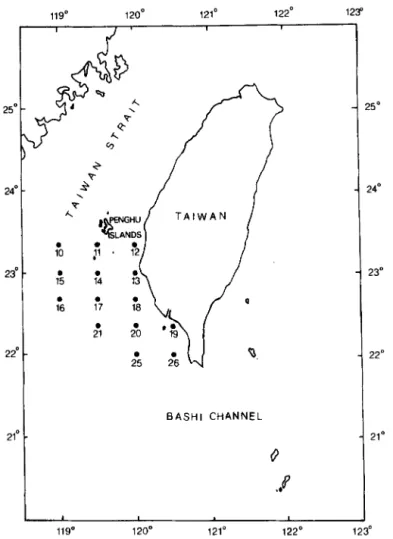
25' 24' 23' 22l 21 BASH1 CHANNEL 0 .P 1 I 119O 120° 12v 122O 1 23 !4" 23" 22" 21U D
Figure 1. Map showing sampling locations in the southern Taiwan Strait.
branch of Kuroshio, also a warm current, passes through Bashi Channel and flows north-
ward into the southern strait along the coast with relatively higher temperature and salinity. During autumn and winter this current encounters the southward flowing cold China Coastal Current in the vicinity of Penghu Islands and is then diverted south- westward into the South China Sea. Upwelling of deep water frequently occurs in late autumn and winter in the study area due to the interaction of waters flowing from opposite directions, the abrupt change of bottom topography, or the drift of surface water driven by strong north-east monsoon winds. Additionally, a large quantity of freshwater is dis- charged into the sea along the western coast, particularly in the rain and typhoon seasons from May to September. The consequent physical and chemical variability in those waters clearly influences the distribution patterns of marine organisms in the southern Taiwan Strait.
At the present time very little is known about phytoplankton in the southern Taiwan
Strait. In a previous study the author investigated the seasonal standing crop and com- munity structure of phytoplankton of this region (Huang, 1986), and in the present work particular attention has been given to the influence of hydrography on phytoplankton distribution using multivariate techniques.
InfZuence of hydrography on the distribution ofphytoplankton 645
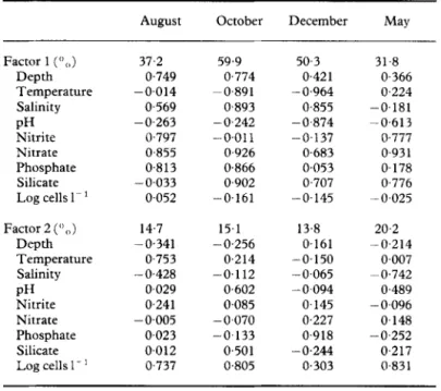
TABLE 1. Factor loadings on hydrographic parameters and cell densities in different months
August October December May
Factor 1 (“(,) 37.2 59.9 50.3 31.8 Depth 0.749 0,774 0,421 0.366 Temperature -0.014 -0,891 - 0,964 0.224 Salinity 0569 0,893 0,855 -0.181 PH -0.263 -0,242 -0.874 -0,613 Nitrite 0.797 -0.011 -0.137 0,777 Nitrate 0,855 0.926 0.683 0,931 Phosphate 0.813 0.866 0.053 0.178 Silicate -0.033 0,902 0.707 0,776 Log cells 1~ 1 0.052 -0.161 -0.145 -0.025 Factor 2 (‘) ,)) Depth Temperature Salinity PH Nitrite Nitrate Phosphate Silicate Log cells I- ’ 14.7 15.1 13.8 20.2 -0.341 -0.256 0.161 -0,214 0.753 0.214 -0.150 0.007 - 0,428 -0,112 -0.065 -0.742 0.029 0,602 -0.094 0.489 0,241 0.085 0.145 - 0.096 - 0.005 -0.070 0.227 0.148 0.023 -0.133 0.918 -0,252 0,012 0,501 -0.244 0.217 0.737 0.805 0.303 0.831
Materials and methods
The locations of 14 sampling stations off the south-western coast of Taiwan are shown
in Figure 1 Some or all were visited on four occasions during the cruises of Ocean
Researcher I from August 1985 to May 1986. On each visit the temperature and salinity of
the water were recorded using a CTD instrument before the water was sampled. The light transmittance in water was determined with both a Secchi disc and a Li-Cor 185 desk unit equipped with an underwater sensor. At each station waters at depths of 3,10,25,50,75 and 1OOm to the surface were collected separateiy with Niskin samplers. For phyto- plankton studies, 1-l subsamples of water were preserved immediately after collection with Lugol’s solution and stored in plastic bottles. The procedures of sample preparation and microscopic examination have been described previously (Huang, 1986). For nutrient study, water samples were stored at 5°C until they were analysed in the laboratory (not later than 10 days after collection). The detailed results of analysis have been reported in Hung et al. (1986), and these records of nutrient concentrations were used in the present study for comparison with phytoplankton data.
In the present study, statistical techniques were employed for both phytoplankton and hydrography data in order to simplify the complicated information and to allow easier interpretation of the variability within hydrographic and phytoplankton data. Factor analysis (Blackith & Reyment, 1971; Joreskog et aI., 1976), a multivariate method of data reduction, is primarily used in the present study. In this analysis, all the relationships among variables are accounted for by relatively independent and interpretable, but nonobservable, factors. In order to simplify interpretation, it is common practice to rotate the factor axes after they have been established. The factor axes were rotated in an oblique process to a new position such that they best accorded with any distinct clusters of vectors
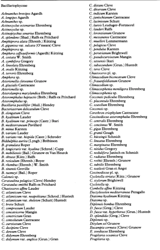
TABLE 2. List of phytoplankton taxa in the study area Bacillariophyceae
Achnanthes brevipes Agardh A. longipes Agardh Achnanthes sp.
Actinocyclus octonarius Ehrenberg Actinocyclus sp.
Actinoptychus senarius Ehrenberg A. splendens (Shad.) Ralfs ex Pritchard Amphiprora alata (Ehrenb.) Kiitzing A. gigantea var. sulcata (O’meara) Cleve Amphiprora sp.
Amphora coffeaeiformis (Agardh) Kiitzing A. costata W. Smith A. cymbifera Gregory A. lineolata Ehrenberg A. ovalis Kiitzing A. terroris Ehrenberg Amphora sp.
Asterionella cleveanus Grunow A. glacialis Castracane Asterionella sp.
Asterolampra marylandica Ehrenberg
Asteromphalus heptactis (Brib.) Ralfs ex Pritchard Asteromphalus sp.
Bacillaria paxillifer (Mull.) Hendey Bacteriastrum delicatulum Cleve B. elongatum Cleve
B. hyalinum Lauder
B. hyalinum var. princeps (Castr.) Ikari B. mediterraneum Pavillard
B. minus Karsten B. varians Lauder
B. varians var. hispida (Castr.) Schroder Biddulphia aurita (Lyngb.) Brebisson B. granulara Roper
B. longicruris var. hyalina (Schrod.) Cupp B. mobiliensis (Bail.) Grunow ex Van Heurck B. obtusa (Kiitz.) Ralfs
B. reticulum (Ehrenb.) Boyer B. rhombus (Ehrenb.) W. Smith B. sinensis Greville
B. tuomeyi (Bail.) Roper Caloneis sp.
Cerataulina pelagica (Cleve) Hendey Cerataulus smithii Ralfs ex Pritchard Chaetoceros afine Lauder
C. atlanticum Cleve
C. atlanticum var. neapolitana (Schrod.) Hustedt C. atlanticum var. skeleton (Schutt) Hustedt C. breve Schutt C. compressum Lauder C. concavicorne Mangin C. constricturn Gran C. convolutum Castracane C. curvisetum Cleve C. decipiens Cleve C. densum Cleve C. didymum Ehrenberg
C. didymum var. anglica (Grun.) Gran
C. distans Cleve C. diversum Cleve C. indicum Karsten C. janischianum Castracane C. laciniosum Schutt C. laevis Leuduger-Fortmorel C. lauderi Ralfs C. lorenzianum Grunow C. messanense Castracane C. muelleri Lemmermann C. pelagicus Cleve C. pendulus Karsten C. peruvianum Brightwell C. pseudocurvisetum Mangin C. setoensis Ikari
C. subsecundum (Grun.) Hustedt C. teres Cleve
Chaetoceros pl. sp.
Climacodium biconcavum Cleve C. frauenfeldianum Grunow Climacodium sp.
Climacosphenia moniligera Ehrenberg Climacosphenia sp.
Cocconeis pediculus Ehrenberg C. placentula Ehrenberg C. scutellum Ehrenberg Cocconeis sp.
Corethron criophylum Castracane Coscinodiscus asteromphalus Ehrenberg C. centralis Ehrenberg C. concinnus W. Smith C. gigas Ehrenberg C. granii Gough C. kiitzingii Schmidt C. lineatus Ehrenberg C. marginatus Ehrenberg C. nitidus Gregory
C. nodulifera Janisch ex Schmidt C. radiatus Ehrenberg
C. rothii (Ehrenb.) Grunow C. subtilis Ehrenberg C. wailesii Gran et Angst Coscinodiscus pl. sp.
Cyclotella striata (Kiitz.) Grunow C. stylorum Brightwell
Cyclotella sp. Cymbella a&e Kiitzing
Dactyliosolen mediterraneus Peragallo Diatoma hyalinum Kiitzing
Diatoma sp.
Diploneis bombus Ehrenberg D. fusca (Greg.) Cleve
D. fusca var. hyperborea (Grun.) Hustedt D. splendida (Greg.) Cleve
Diploneis sp. Ditylum sol Grunow
Eucampia cornuta (Cleve) Grunow E. zoodiacus Ehrenberg
Fragilaria oceanica Cleve Fragilaria sp.
Injluence of hydrography on the distribution of phytoplankton
TABLE 2. (Continued)
Gomphonema sp. Gossleriella tropica Schutt
Grammatophora marina (Lyngb.) Kiitzing Guinardiaflaccidu (Castra.) Peragallo Gyrosigma balticum (Ehrenb.) Cleve Gyrosigma sp.
Hernia&us hauckii Grunow ex Van Heurck H. sinensis Greville
Hemidiscus sp.
Hyalodiscur stelliger Bailey H. subtilis Bailey
Lauderia borealis Gran Lepcocylindrus danicus Cleve Licmophora abbreviata Agardh Licmophora sp.
Lithodesmium undulatum Ehrenberg Mastogloia sp.
Melosira distans (Ehrenb.) Kiitzing M. jurgensii Agardh
M. moniliformis (Mull.) Agardh M. nummuloides (Dillw.) Agardh Melosira sp.
Navicula angusta Grunow N. cancellata Donkin N. ciauata Gregory N. directa (W. Sm.) Cleve N. distans (W. Sm.) Cleve N. forcipata Greville N. humerosa Brebisson N. lanceolata (Agardh) Kiitzing N. membranacea Cleve N. monilifera Cleve N. perrhombus Hustedt
N. tuscula (Ehrenb.) Van Heurck Navicula pl. sp.
Nitzschia acuminata (W. Sm.) Cleve N. angularin W. Smith
N. closterium (Ehrenb.) W. Smith N. delicatissima Cleve
N.fonticola Grunow N.frustuIum (Kiitz.) Grunow N. gracilis Hanrzsch N. hungarica Grunow N. lonceolata W. Smith N. littoralis Grunow
N. longissima (Breb.) Ralfs ex Pritchard N. longissima var. reversa Grunow N. marginulata Grunow
N. marina Grunow N. panduriformis Gregory
N. panduriformis var. intermedia Grunow N. seriata Cleve
N. srgnra (Kutz.) W. Smith N. sigma var. intermedia W. Smith N. spathrrluta Brebisson ex W. Smith N. rryblionella Hantzsch
N. vttrea Norman Nitzschia pl. sp.
Par&z sulcata (Ehrenb.) Cleve Pmnrrlaria sp.
Planktoniella sol (Wall.) Schutt Pleurosigma afine Grunow
P. angulatum var. strigosa (W. Sm.) Cleve P. fasciola (Ehrenb.) W. Smith
P. intermedium W. Smith P. nnviculaceum Brebisson P. normani Ralfs P. pelagicum Peragallo
P. rigidum var. incurvata Grunow P. strigosum W. Smith
Pleurosigma sp.
Podosira stelhger (Bail.) Mann Rhabdonema ndriaticum Kiitzing R. arcuatum (Lyngb.) Kiitzing Rhizosolenia acuminata (Perag.) Gran R. alata Brightwell R. bergonii Peragallo R. castracanei Peragallo R. crassispinu Schroder R. cylindrus Cleve R. delict&a Cleve R. fragilissimn Bergon R. hebetata Bailey R. imbricata Brightwell R. robusta Norman ex Pritchard R. setigera Brightwell
R. stolterfothii Peragallo R. styliformis Brightwell
R. styliformis var. latissima Brightwell Rhizosolenia sp.
Schroederella delicatula (Perag.) Pavillard Skeletonema costatum (Grev.) Cleve Stauroneis amphioxys Gregory
Stephanopyxis nipponica Gran et Yendo S. palmeriana (Grev.) Grunow Stigmophira rostrata Wallich
Striateha unipunctata (Lyngb.) Agardh Surirellu amoricana Peragallo
S. fastuosa Ehrenberg Surirella sp.
Synedra fasciculata (Agardh) Kiitzing S. gaillonii (Bory) Ehrenberg S. ulnu (Nitzsch) Ehrenberg S. ulna var. danica (Kiitz.) Grunow Synedra sp.
Thalassionema nitzschioides Hustedt Thalassiosira baltica (Grun.) Ostenfeld T. condensata Cleve
T. decipiens (Grun.) Jorgensen T. eccentrica (Ehrenb.) Cleve T. gravida Cleve
T. hyalina (Grun.) Gran T. nordenskiold Cleve T. pacifica Gran et Angst T. rotula Meunier Thnlassiosira pl. sp.
Thalassiothrix frauenjeldii Grunow T. Iongissimu Cleve et Grunow T. mediterranea var. pacifica Cupp Trachyneis aspera (Ehrenb.) Cleve
TABLE 2. (Continued) T. aspera var. elliptica Hendey
Triceratium favus Ehrenberg T. formosum Brightwell T. reticulum Ehrenberg Triceratium sp. Dinophyceae
Ceratium candelabrum (Ehrenb.) Stein C. furca (Ehrenb.) Claparede et Lachmann C. lineatum (Ehrenb.) Cleve
C. macroceros var. gallicum (Kof.) Jiirgensen C. massiliense (Gourr.) Jiirgensen
C. pentagonum Gourret C. teres Kofoid Ceratium pl. sp.
Cladophyxis brachiolata Stein Cochlodimium sp.
Dinophysis sp.
Glenodinium foliaceum Stein Glenodinium sp.
Gonyaulax polygramma Stein G. turbynei Murray et Whitting Gymnodinium arcuatum Kofoid G. ochraceum Kofoid et Swezy G. rhomboides Schutt G. sanquineum Hirasaka G. vestifici Schutt
Gymnodinium sp.
Gyrodinium spirale (Bergh) Kofoid et Swezy Noctiluca scintillans (Macartn.) Ehrenberg Ornithocercus sp.
Oxytoxumgladiolus Stein 0. scolopax Stein
0. reticulatum (Stein) Butschi
0. tesselatum (Stein) Schutt Oxytoxum sp.
Prorocentrum micans Ehrenberg P. triangulatum Martin
P. rriestinum Schiller
Protoperidinium abei (Abe) Paulsen F’. achromaticum (Lev.) Balech P. balticum (Lev.) Lemmermann P. cerasus (Pa&) Balech P. decipiens (Jorg.) Parke ef Dodge 2’. depressurn (Bail.) Balech P. faeoceros Paulsen P. granii (Ost.) Balech P. islandicum (Pauls.) Balech P. marukawai Abe
P. oceanicum (Vanhoffen) Balech P. pentagonum (Gran) Balech P. pyriforme (Pauls.) Balech P. subinerme (Pauls.) Loeblich III P. thorianum (Pauls.) Balech Protoperidinium sp. Pyrocystis lunula Schutt P. lanceolata Murray P. noctiluca Murray
Scrippsiella trochoidea (Stein) Loeblich Warnowia parva (Lohm.) Lindemann Prymnesiaceae
Chrysochromulina sp. Chrysophyceae
Dictyocha fibula Ehrenberg
Distephanus speculum (Ehrenb.) Hackel
Mesocena sp. Cyanophyceae Anabaenasp.
Pelagothrix clevei Schmidt Richelia intracellularis Schmidt Spirulina sp.
Trichodesmium contortum Wille T. erythraeum Ehrenberg T. thiebautii Gomont
representing variables (Harbaugh & Merriam, 1968; JGreskog et al., 1976). Because a large
number of species occurred only occasionally and did not offer much useful ecological
information, a criterion of selection of species was established before computation. A
species selected for the analysis had a frequency of occurrence in greater than 15 yO of the
total samples in the whole year’s collections, irrespective of its abundance in particular
samples. In addition, the variability caused by the absence of species included in the
analysis was reduced by using logarithmic transformation of counting values (Estrada &
Blasco, 1979). That is X-+log(X+ l), where Xis the number of a species in 11 of seawater.
However, this transformation was not applied to hydrographic data. Multiple-regression
and cluster analysis were also done on transformed data as an aid to the interpretation of
phytoplankton distribution.
Results and discussion
Analysis of hydrographic data
Preliminary factor analysis based on 287 samples of entire collections yielded the first two most important factors, however, these factors did not explain as much variability as
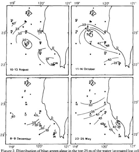
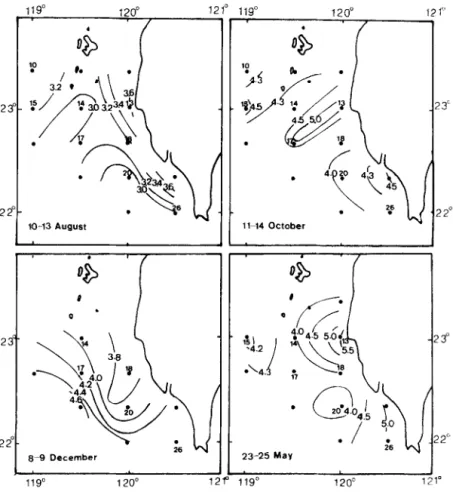
Influence of hydrography on the distribution of phytoplankton 649 1 l-14 October lo-13 August 1 119" 120" 121" 119" 120" 121' I 23" / L 21" . 220 23-25 May Ilg 120" 121
Figure 2. Distribution of blue-green algae in the top 25 m of the water (averaged log cell numberl-‘).
expected, nor did the seasonal sequence of distribution. For this reason the subsequent
factor analysis was done on the data collected on individual cruises (Table 1). Obviously,
loadings on hydrographic parameters were variable with season. The first two factors
explained more than 5 1” 0 of total variability. For factor 1, the loading on temperature was
extremely low in August because the whole strait water was occupied by northward
flowing warm currents in summer (Chu, 1963; Fan, 1982). With October data, factor 1
accounted for 60?(, of total variability. This factor is referred to as the water-mass factor
that can be deduced from high negative loading on temperature and positive loadings on
salinity and nutrients. Furthermore, the high loading on depth suggested the stratification
of waters in the study area. The result of the following Q-model factor analysis (Harbaugh
& Merriam, 1968; Klovan & Imbrie, 1971; Jijreskog et al., 1976), correlating hydro-
graphic environments in terms of the phytoplankton species composition which they
possess, supports this phenomenon. However, the present factor analysis failed to demon-
strate the variability explained by the high-temperature and high-salinity Kuroshio
water. It could be that Kuroshio water gradually loses its characteristics as it enters the
strait and mixes with other waters. The influence of water mass on the factor I became very
evident during the winter period, yet the upwelling determined from T-S and nutrient
diagrams (Fan, 1982; Hung et al., 1986) was not detectable. The fact is that the upwelling
lo-13 August 11-14 October
I
I
I
I I
I
.I
I
8-Q December l 23-25 May 26 Y
-L
119 P 120° 12P 116 120° 121°
Fig&3. Distribution of temperatures in the top 25 m of the water (“C).
whole study area. Correlation between upwelling and phytoplankton distribution has also been shown by Estrada and Blasco (1979), Blasco et al. (1980) and Estrada (1984) using principal-component analysis. In May, pH and nutrients, which relate to biological activity, accounted for the largest portion of the total variability.
Factor 2 accounted from 13+3-20.2% of the total variability (Table 1). This factor, except in December, was strongly influenced by algal activity represented mainly by the
blue-green alga. Pelagothrix clevei in August and diatoms Thalassionema nitzchioides,
Thalassiothrixfrauenfeldii, Thalassiosira condensata, T. rotula and Bacteriastrum hyalinum in October. In May, high positive loading on algal density and negative loading on salinity indicated that the discharge of freshwater into the sea was important to algal distribution, particularly in the coastal area.
In the factor analysis, high loadings on both phytoplankton density and hydrographic parameters for the same factor do not necessarily mean that they were significantly correlated. In the present study their correlation was determined by multiple regression with the stepwise method at p < 0.05 using the F-test. It appeared that temperature was the sole parameter influencing algal abundance in August, whilst both temperature and salinity were important to algal distribution in October and December. The spring out- burst of phytoplankton was closely related to pH, salinity, silicate, depth and nitrate. The above results agree with those of the previous factor analysis in the explanation of seasonal variations of hydrography and phytoplankton.
Influence of hydrography on the distribution of phytoplankton 651
IO-13 August
23"
11-14 October
Figure 4. Distribution of diatoms and dinoflagellates in the top 25 m of the water (averaged log cell number I- ‘).
Phytoplankton assemblages in the study area
A total of more than 300 species and varieties of phytoplankton were obtained from the study area, of which 255 species were diatoms and 55 and seven species were dino- flagellates and blue-green algae, respectively (Table 2). The flora did not change signifi- cantly as compared with that in the previous year (Huang, 1986). A large number of species occurred in less than 15 of all samples and accounted for less than 20°, of all the standing crop in cell numbers. These rare species contributed very little ecological infor-
mation to the present study. Whilst species of Bacteriastrum, Chaetoceros, Coscinodiscus
and Thalassiosira, Thalassionema nitzschioides and Thalssiothrixfrauenfeldii were the most abundant in the populations; they contributed from 5”,, to 15”,, of the total standing crops. In summer and autumn, higher standing crops of phytoplankton at some stations often represented a higher proportion of blue-green algae to diatoms and flagellates, The
main blue-green algae were Pelagothrix clevei and Trichodesmium erythraeum. Very few
dinoflagellates and other small flagellates were observed in the samples; most of them were Protoperidinium, Glenodinium and Ceratium.
Maximum standing crops of phytoplankton occurred in October and May due to the outgrowth of certain species of blue-green algae and diatoms. The majority of phyto- plankton appeared in the water layer within 25 m of the surface. The light intensity at 25 m
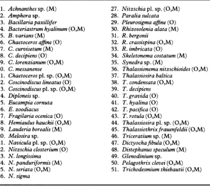
TABLE 3. Phytoplankton occurring in at least 15% of all samples; taxa selected for monthly factor analysis (0, October; M, May)
1. Achnanthes sp. (M) 2. Amphora sp. 3. Bacillaria pa&lifer 4. Bacteriastrum hyalinum (0,M) 5. B. varians (M) 6. Chaetoceros afine (0) 7. C. curvisetum (M) 8. C. decipiens (0) 9. C. lorenzianum (0,M) 10. C. messanense 11. Chaeroceros pl. sp. (0,M) 12. Coscinodiscus lineatus (0) 13. Coscinodiscus pl. sp. (0,M) 14. Diploneis sp. 15. Eucampia cornuta 16. E. zoodiacus 17. Fragilaria ocenica (0) 18. Hernia&s hauckii (0,M) 19. Lauderia borealis (M) 20. Melosira sp. 21. Navicula pl. sp. (0,M) 22. Nitzschia closterium (0) 23. N. longissima 24. N. pandurtformis (M) 25. N. seriata (0,M) 26. N. sigma 27. Nitzschia pl. sp. (0,M) 28. Paralia sulcata 29. Pleurosi’a afine (0) 30. Rhizosolenia alata (M) 31. R. bergonii 32. R. crassispina (0,M) 33. R. imbricata (0) 34. Skeletonema costatum (M) 35. Synedra sp. (M) 36. Thalassionema nitzschioides (0,M) 37. Thalassiosira baltica 38. T. condensata (0,M) 39. T. decipiens 40. T. gravida (0) 41. T. hyalina (0) 42. T. pacifica (0) 43. T. rotula (0,M) 44. Thalassiosira pl. sp. (0,M) 45. Thhlassiothrixfrauenfeldii (0,M) 46. Triceratium sp. (M) 47. Dictyochahbula (0,M) 48. Distephanus speculum (M) 49. Glenodinium sp. 50. Pelagothrix clevei (0,M) 5 1. Trichodesmium thiebautii (0,M)
of most sampling stations decreased less than 10% of the incident light at the surface.
Therefore, algal densities in the upper 25 m were used to illustrate the distribution pattern
of phytoplankton. From Figure 2 it can be seen that blue-green algae and diatoms
appeared in the north-westward direction off the south-west coast of Taiwan which is
consistent with the movement of the Kuroshio and South China Sea currents (Figure 3).
Maximum amounts were found at station 14 in October and at station 20 in May,
respectively. The close relationship between temperature and blue-green alga distri-
bution has been indicated previously (Huang, 1986). Figure 4 shows that both diatoms
and dinoflagellates were abundant at stations 13,14,15,17 and 26 in these two months. In
December, the cold water moved down from the north as shown in Chu (1963), Fan (1982)
and Figure 3, and so most phytoplankton occurred southward of and near station 25.
During the summer period the phytoplankton were relatively homogenous in the study
region.
Analysis of phytoplankton data
From the whole year’s collections, 51 taxa (Table 3) were selected for both factor and cluster analyses. These species occurred in at least 15% of all samples (287), regardless of
their abundance. In the preliminary results of the factor analysis based on the entire data
most species which were dominant throughout the year did not contribute significantly to
the variability; therefore, they reduced the seasonal variation. In order to avoid the multi-
month variability as shown in Estrada (1984), and to facilitate interpretation, the sub-
sequent factor analysis was based on each of the monthly collections. Twenty-seven
Influence of hydrography on the distribution of phytoplankton 653 I,0 Factor I 0,s I R.lmN
P
b
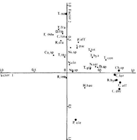
Paff .Figure 5. The positions of 27 species vectors on the first two factors produced from October assemblages. Abbreviations refer to the species names in Table 3.
the analysis. These species occurred in at least 200,, of all samples taken on each cruise. Figure 5 clearly shows three clusters of species strongly influencing the first two axes in
October. Chaetoceros &ine together with C. decipens, C. lorenzianum, Chaetoceros sp. and
Bacteriastrum hyalinum, form a cluster and accounted for the major portion of the total variability of factor 1. Examination of the basic data showed that these taxa were plentiful
in observed assemblages, especially at station 13. Thalassionema nitzschioides, which was
abundant in the offshore area of stations 15 and 16, formed the second cluster and strongly
influenced factor 2. The third cluster was occupied by Pelagothrix clevei only in the
negative side of factor 2; this is an alga which predominated at station 14. The rest of the species contributed relatively less variability to the first two factors. With May data
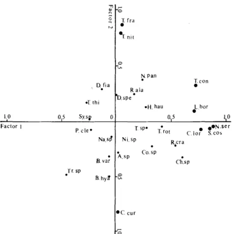
(Figure 6) Nitzschia seriata, Skeletonema costatum, Chaetoceros lorenzianum, Thalassiosira
condensata and Lauderia borealis strongly influenced factor 1, and Thalassiothrix
frauenfeldii, Thalassionema nitzschioides and Chaetoceros curvisetum influenced factor 2 in opposite directions. These diatoms were dominant at station 12,13,19 and 26. Blue-green algae explained the lower May variability, although they were abundant at station 20. The above results revealed seasonal and spatial variations of the main taxa. Nevertheless, in multivariate analysis phytoplankton species which have high loadings in the same cluster
may not necessarily occur together frequently (Maddock et al., 1981). Therefore,
interpretation of the results of the analysis must be made with caution.
The geographic pattern of phytoplankton distribution can be detected when seasonal variation is removed from the multivariate analysis (Matta & Marshall, 1984). In the
, Dfia . % thi 1.0 Factor I O.,S sy.sp 0 P. cle- N&S? B.vnf Tr. SP . B. hy8 p.Pan icon R-ala b.spe
l ti. hau L bor
l .
0.5 I,0
T SP.
T:rot C. lor . .qu.ser S.cos Ni.sp 2.sp co. iP Ricra C&P DC. cur ,- 0
Figure 6. The positions of 27 species vectors on the first two factors assemblages. Abbreviations refer to the species names in Table 3.
produced
TABLE 4. Loadings of the first factor on sampling stations and depths in October and May Station No. 3 October 1985 May 1986 10 25 3 10 25 10 11 12 13 14 15 16 17 18 19 - 20 21 25 - 26 0.125 0.116 0.092 0.113 0.028 0.088 0.666 0.422 0.607 0.777 0.766 0.847 0.833 0.924 0.847 0.079 0.185 0.656 0.710 0.873 0.757 0.223 0.299 0.607 0.850 0.722 -0.068 .0.133 - -0.141 0.095 0.345 - 0.083 0.688 0,512 0.840 0.908 -0-048 0.822 0.144 0.190 0.398 0.342 - -0.108 -0.089 0.362 -0,043 0,141 0.730 0.791 0.046 0.922 0.945 O-833 0,481 0.327 -0.071 0,290 -0.182 0,183 0.618 0.947 0.027 0.943 0.767 0.882 0.522 - -0,048 0,135 0.843 0.069 0.657 0.825 0.891 -0.110 0.944 0.941 0.942 0,214
Influence of hydrography on the distribution ojphytoplankton 655
statton Depth(m)
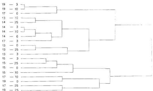
Figure 7. Dendrogram showing clusters of phytoplankton populations collected from different depths at five stations in October 1985.
Q-model analysis, based on 5 1 taxonomic groups, the variabilities explained by locations
were evidently different. It appears that stations 13,14,16 and 21 had higher cell densities
(Figure 4) and, therefore, contributed a larger portion of variability to factor 1 in October,
whilst stations 20, 21, 25, 17 and 18 accounted for the variability in May (Table 4).
According to the species composition of assemblages, the former can be referred to as the diatom factor and the latter as the blue-green alga factor. In addition, highly variable loadings with depths were also found in some small areas, for example at stations 18 and 25
in October and at stations 14 and 16 in May. It is of particular interest that loadings at
3 and 10 m at station 18 were very high, but negligible at 25 m in October. This was
probably related to the upwelling of deep water to the subsurface layer (the tempera-
ture at 25 m was more than 2°C lower than at the surface) as shown in Hung et al.
(1986). Therefore, the vertical variability of the phytoplankton population can reflect
stratification or vertical movement of water in certain areas.
The close relationship between the species composition of phytoplankton and water
movement has been shown previously (Estrada & Blasco, 1979; Estrada, 1984). The
similarity between two algal populations can be determined on the basis of the species
present. Thus it can be assumed that the higher the similarity between two phytoplankton
populations, the closer the characteristics of the two water regimes. Because of the very
complicated hydrography in October, phytoplankton populations at five major stations in
that month were examined by grouping into clusters based on 5 1 taxonomic groups (Table 3). The results of both the factor and the cluster analyses were quite similar. As shown in the dendrogram of cluster analysis (Figure 7), four clusters appeared in the last three large distances. Populations at stations 13 and 14 combined into a cluster, while those at station 15 in the offshore area formed an isolated cluster. The first cluster appeared in the high-
temperature regime (27.0*0.3”C) that was possibly a mixture of Kuroshio and local
influence of the southward flowing China Coastal Current. Examination of the species composition of clusters also showed different major taxa. Separate clustering of stations 17 and 19 at both ends of the dendrogram was attributed to the discontinuity of water movement, which again resulted from the upwelling near two stations as mentioned above.
It is concluded that multivariate analysis provides ecologically significant information in the interpretation of phytoplankton distribution under the influence of hydrography. Vertical, spatial and temporal variabilities of small-scale data (monthly collections) were apparent in the present study. The above results show that the distribution of different phytoplankton populations can be a useful tracer of water movement.
Acknowledgements
Thanks are due to the crew of R/ V Ocean Researcher I for their kind assistance during the
cruises and to Mr Chang J. H. and Miss Cheng C. Y. for microscopic examination and data analysis. I am greatly indebted to Dr Hung T. C. for his kindness in providing me with nutrient data. This study was financially supported by the National Science Council of the Republic of China.
References
Black&, R. E. & Reyment, R. A. 1971 Multivariate Morphometrics. Academic Press, London.
Blasco, D., Estrada, M. & Jones, B. 1980 Relationship between the phytoplankton distribution and composition and the hydrography in the northwest African upwelling region near Cabo Corbeiro. Deep-Sea Research 27A, 799-821.
Chu, T. Y. 1963 The oceanography of the surrounding waters of Taiwan. Report of the Institute of Fishery Biology of the Ministry of Economic Affairs and National Taiwan University 1,29-39.
Estrada, M. 1984 Phytoplankton distribution and composition off the coast of Galicia (northwest of Spain). Journal of Plankton Research 6,417-434.
Estrada, M. & Blasco, D. 1979 Two phases of the phytoplankton community in the Baja California upwelling. Limnology and Oceanography 24,1065-1080.
Fan, K. L. 1982 A study of water masses in Taiwan Strait. Acta Oceanographica Taiwanica 13,140-153. Harbaugh, J. W. & Merriam, D. F. 1968 Computer Applications in Stratigraphic Analysis. Wiley, London. Holligan, P. M., Maddock, L. &Dodge, J. D. 1980 The distribution of dinoflagellates around the British Isles
in July 1977: a multivariate analysis. Journal of the Marine Biological Association of the United Kingdom 60,851-867.
Huang, R. 1986 Phytoplankton distribution off the southwestern coast of Taiwan. Acta Oceanographica Taiwanica 16,103-l 16.
Hung, T. C., Tsai, C. C. H. & Chen, N. C. 1986 Chemical and biomass studies: (1) Evidence ofupwelling off the southwestern coast of Taiwan. Acta Oceanographica Taiwanica 17,29-44.
Joreskog, K. G., Klovan, J. E. & Reyment, R. A. 1976 Geological Factor Analysis. Elsevier Scientific Publishing Company, Amsterdam.
Klovan, J. E. & Imbrie, J. 1971 An algorithm and FORTRAN IV program for large-scale Q-mode factor analysis. Mathematical Geology 3,61-67.
Maddock, L., Boalch, G. & Harbour, D. S. 1981 Populations of phytoplankton in the western English Channel between 1964 and 1974. Journal of the Marine Biological Association of the United Kingdom 61, 565-583.
Matta, J. F. & Marshall, H. G. 1984 A multivariate analysis of phytoplankton assemblages in the western North Atlantic. Journal of Plankton Research 6,663-675.
Mall, R. A. & Rohlf, F. J. 1984 Analysis oftemporal and spatial phytoplankton variability in a Long Island salt marsh.3ournal of Experimental Marine Biology and Ecology 51,133-144.