1. Introduction
The funded project contains two parts; one is to coordinate and service the individual projects of program of Variations of Northern SCS (VANS) and its joint project Windy Island Soliton Experiment (WISE) which funded by the Office of Navy Research (ONR) of United State of American. The primary works include to host a workshop at Taipei made a workable plan and to execute the field work. The workshop has been taken place at Taipei on October 25-27, 2004. The progress and conclusion of the workshop will be stated in Section 2. The primary field work started early April 2005 and ended May 2005. The work is quite successful and will be illustrated in Section 3.
The personal research project is to study the intra-seasonal variation in the northern SCS and Luzon Strait using the previous and new mooring
measurements. Two papers has been in press in the international journal and several papers are in preparation. The new measurement has been started. A mooring array from Luzon Strait to the shelf of northern SCS has been deployed in late April 2005. The mooring work is cooperated with the
scientists of USA. The array will be kept in the water for a year, but it will be refurbished every 3 months. This part of work is reported in Section 3. Two papers, which have been accepted for publication in international journal, are listed in Section 4 as a preliminary result. Section 5 provides a short
summary for the work from August 2004 to May 2005. 2. Workshop
The workshop was taken place on Oct 25-27, 2004 at campus of National Taiwan University. The meeting schedule as shown in Table 1.
Monday, October 25
Opening Session - Professor Tswen-Yung David Tang, Presiding
8:30
Keynote Speaker 1 Prof. Char-Shine Liu, Director
National Center for Ocean Research Keynote Speaker 2 Dr. Theresa Paluszkiewicz,
Program Officer Office of Naval Research
Session 1 - Review of Scientific and Logistical Issues Dr. Steve Murray and Prof. Wen-Ssn Chuang,
Presiding 9:10
Questions Raised
Profs. Steve Ramp and Ching-Sang Chiu
Internal bores in the Luzon Strait - Moored Observations
Profs. Wen-Ssn Chuang and W.-D. Liang
Overview of Taiwan's Ship and Staging Capabilities Profs. Ruey-Chang Wei and David Tang
10:10 TEA AND COFFEE BREAK
Session 2 -Research Team Intentions - Modeling and Remote Sensing
Dr. Linwood Vincent and Prof. Wen-Ssn Chuang, Presiding
10:40
Non-Hydrostatic Modeling
Profs. Shenn-Yu Chao and Ping-Tung Shaw
The Naval Research Laboratory (NRL) Model Dr. Dong-Shang Ko
Satellite Remote Sensing
Dr. Tony Liu and Prof. Ming-Kuang Hsu
Ship Observation and MODIS Images
Dr. Yiing Jang Yang, Ming-Huei Chang and Kai-Chieh Yang
12:00 LUNCH
Session 3 - Research Team Intentions - Interdisciplinary
Dr. Ellen Livingston and Prof. Chifang Chen, Presiding
13:00
The WISE/VANS Moored Array Profs. Steve Ramp, C.-S. Chiu, and Y.J. Yang
The Shallow Water Physical Oceanography Experiment
Dr. Glen Gawarkiewicz and Prof. Joe Wang
Water PO Experiment Prof. Louis St. Laurent
The Shallow Water Acoustic Propagation Experiment Prof. Ching-Sang Chiu, Prof. Chifang Chen, Dr. Phil
Abbot
14:20 TEA AND COFFEE BREAK
Session 4 - Research Team Intentions - Deep Water Dr. Steve Murray and Prof. Cho-Teng Liu, Presiding
15:00
Multi-ship Surveys Near the Luzon Strait Prof. Cho-Teng Liu
Philippine Research Plans for 2005-2006 Profs. Cesar Villanoy and Gil Jacinto
Shipboard Tracking of Soliton Packets in the NE South China Sea
Dr. Rob Pinkel
Nonlinear Internal Wave Observations Using Lagrangian Floats
Profs. Eric D'Asaro and Ren-Chieh Lien
Internal Wave Velocity Profiles From Wind Drifters in the SCS
Drs. Peter Niiler and Luca Centurioni
16:40 DAY CONCLUDES
18:00
BANQUET - Hosted by the Taiwan National Science Council
Invitations with directions will be provided
Tuesday, October 26
This day is devoted to working groups and discussion
9:00
Logistical Support Requirements Review Ship Schedule (Tang/Ramp) Accommodations, transportation, infrastructure in
Requirements for dockside support (all PIs) Storage Space
Work Space
Trucks/Loading Equipment, etc.
10:00 TEA AND COFFEE BREAK
10:00
Small Breakout Groups Moorings SW
Experiment
Luzon
Area Modeling
Ramp Chiu CT Liu Chao
Tang Chen Lien Shaw
Yang Abbot D'Asaro Ko
T. Liu Gawarkiewicz Pinkel Chuang
Hsu Wang Niiler Liang
Reeder St. Laurent Centurioni Wu
Murray Wei Tseng Paluszkiewicz
Livingston Vincent
12:00 LUNCH
13:00 Breakout Groups Continued
15:00 TEA AND COFFEE BREAK
15:30
Working Group Reports Moorings - Ramp/Tang SW Experiment - Chiu/Chen
Luzon Strait - Pinkel/Liu
Modeling - Chao/Wu
18:30
BANQUET - Hosted by the Office of Naval Research of U.S.A
Invitations with directions will be provided
Wednesday, October 27
9:00 Meeting Summary and Action Items
12:00 LUNCH
13:00
Taipei City Tour (free of charge)
Palace Museum
House
Chinese Handicraft Center
The workshop went smoothly as we expected. The attendees came from various originations and had various expertises. Table 2 lists the attendees.
ATTENDEES
organization name organization name
Applied Physics Laboratory, University of Washington Lien, Ren-Chieh Commander Submarine Force U.S. Pacific Fleet Cross, Patrick Florida State
University St. Laurent, Louis
Institute of Marine Science, University of the Philippines David, Laurel Jacinto, Gil Villanoy, Cesar Johns Hopkins University Applied Physics Laboratory Green, Larry Naval Postgraduate School Chiu, Ching-Sang Ramp, Steven R. Reeder, Ben Naval Research Laboratory, Stennis Space Center
Ko, Dong-Shang North Carolina
State University Shaw, Ping-Tung
Oasis Inc. Abbot, Phil Office of Naval Research Chotiros, Nick Curtin, Thomas Fiadeiro, Manny Harper, Scott Livingston, Ellen Murray, Stephen P. Paluszkiewicz, Theresa Vincent, Linwood Office of Naval Research -Tokyo International
Liu, Antony K. Scripps
Institution of Oceanography Centurioni, Luca Klymak, Jody Niiler, Pearn P. Pinkel, Rob
Field Office
University of
Maryland Chao, Shenn-Yu
Woods Hole Oceanographic Institution Gawarkiewicz, Glen Caruso, Michael Chinese Naval Academy
Yang, Yiing Jang (楊 穎堅) Liang, Wen-Der (梁 文德) Lu, Wei-Lee (呂維 理) Chinese Naval Hydrographic and Oceanic Office Kao, Chin-Chung (高 志中) Kuang Wu Institute of Technology Hsu, Ming-Kuang (許明光) National Center for Ocean Rearch Yang, Yih (楊益) National Sun Yat-Sen University Tseng, Ruo-Shan (曾若玄) Liu, James T. (劉祖 乾) Wei, Ruey-Chang (魏瑞昌) Hsu, Rong-Chung John (許榮中) Chen, Peter (陳震遠) National Taiwan Normal University Wu, Chau-Ron (吳朝 榮) National Taiwan Ocean University Hu, Jian-Hwa (胡健 驊) Nation Taiwan University
Tang, Tswen Yung David (唐存勇) Chuang, Wen-Ssn (莊文思) Wang, Joe (王冑) Chern, Ching-Sherng (陳慶 生) Liu, Cho-Teng (劉倬 騰) Chen, Chi-Fang (陳 琪芳) China College of Marine Wang, Chung-Wu (王崇武)
Technology and Commerce
The result of workshop is fruitful. The materials of presentation of each speaker has been stored in our website (http://140.112.68.83/~vans/#agenda, userid:scs, pw:taroko). Four working groups have been identified. The solitary wave group would focus their studies on the solitary wave generation, transformation and dissipation. The impact of solitary wave on the acoustics propagation is also a topic of study in this group. The primary mission of mooring group is to deploy a mooring array from Luzon Strait to shelf of northern SCS. Figure 1 shows the proposed mooring array.
MOORING LOCATION AND TOPOGRAPHY
Figure 1b
The primary studying object is to address the questions of origination of solitary wave, whether the solitary wave is a persistent feature or not, what the
intra-seasonal variation in the central northern SCS is and the characters of South China Sea Warm Current (SCSWC). The above two groups plan using our research vessels to perform the proposed field work. Totally, around 30 days ship-time is requested. The group of Luzon Strait is leaded by Dr. C. T. Liu. I believe he would report the progress of this group. The modeling group is leaded by S. Y. Chao, a professor of University of Maryland. Dr. C. R Wu will work on his basin-wide model joining with Wen-Ssn Chuang, me and several other domestic PIs primarily to investigate the circulation in the northern SCS.
3. Experiment
The main field work has been done at a couple weeks ago. The mooring array has been in the water. The left-over field work is to refurbish the moorings every 3 months. A number of ship measurements have been collected and exchanged between the PIs and joint nations. The data include Conductivity Temperature Depth profiler (CTD) casts, EK500 vertical acoustic data, Radar images, Shipboard Acoustics Doppler Current Profiler (SbADCP) current data, Expendable Bathythermography (XBT), Expendable Conductivity
Temperature Depth profiler (XCTD) data, Expendable Current Profiler (XCP) data, Lagrangian floats, and Scanfish/SeaSoar surveys data. And some Synthetic Aperture Radar (SAR) and Moderate Resolution Imaging
Spectroradiometer (MODIS) satellite images during our survey duration were collected. All of our survey work went smooth and most of the data reveal fairly good quality.
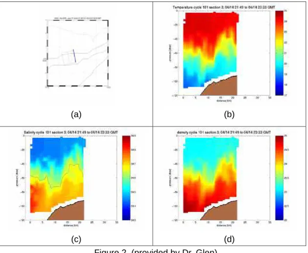
Figure 2. is hydrographic surveys data by deploying Scanfish in OR1 field work duration. The Scanfish was dragged cross-shore in the shelf break northwest of South China Sea. The cruise track is shown in Figure 2a. The cross-shore variations of temperature, salinity, and density are shown in Figure 2b, Figure 2c and Figure 2d respectively. Their vertical structures indicate that mixing layer deepen obviously near shelf break.
(a) (b)
(c) (d)
Figure 2. (provided by Dr. Glen)
Satellite images provide a great help for observations of internal waves propagating. SAR and MODIS images are shown in Figure 3. From Figure 3a, some westward internal solitary waves (ISW) were observed by SAR in
ISWs, MODIS image shown in Figure 3b reveal a group of reflection ISW resulted from interacting with DongSha Island.
(a) (b)
Figure 3.
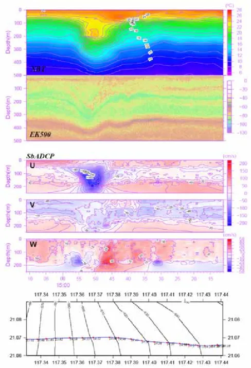
During OR3 survey cruise, we traced ISWs by SbADCP, EK500, XBT, CTD, and Radar. As shown in Figure 4, we followed a huge ISW with ship speed higher than ISW propagating speed upon the shelf near shelf break, and then went across it. Local depth is about 600m there. The ship track is shown in the lowest panel of Figure 4 (The contours indicate isobath, and red points indicate deploying time of XBT). The XBT temperature data, EK500 sound reflective intensity, and SbADCP zonal, meridional, and vertical velocity revealed strong signal coincidently when the ship kept on the wave. From the XBT temperature profile, the influenced depth is up to 500m. Maximum variation of temperature is about 8 °C, and an overturning occurs at depth about 170m. From EK500 data, the vertical displacement could be up to 150m. ADCP zonal velocity could be up to 160 cm/s, and vertical velocity show a downwelling followed by a upwelling with maximum velocity 30 cm/s.
In the continental shelf with depth about 320m farther from shelf break, Yo-Yo CTD was deployed prior to ISW package arrival, which went on up to it passed away. The wave package could be found in Radar image as shown in
Figure 5. In Figure 6, CTD temperature, salinity, and density, EK500, and SbADCP zonal velocity are shown. The character looks different from Figure 4. The wave traced in Figure 4 is single huge wave, and here is a group of waves with smaller variations of property. The huge ISW breaks into a number of small ones when it propagates into shallow water area. The result could be observed by SAR and MODIS images and be explained by theoretical and numerical model. The maximum variation of temperature is about 4°C as shown in temperature profile. From density profile and EK500 data, leading wave vertical displacement is up to 100m and zonal velocity is about 60 cm/s.
Figure 5
GEOPHYSICAL RESEARCH LETTERS, VOL. ???, XXXX, DOI:10.1029/,
Energy and Characteristics of Nonlinear Internal Waves in
South China Sea
R.-C. Lien,1 T. Y. Tang,2 M. H. Chang,2 E. A. D’Asaro,1
Simultaneous ADCP measurements taken in South China Sea (SCS) reveal geographically distinct internal-wave
char-acteristics. (1) West of Luzon Strait, the total
internal-wave energy (Eiw) is 10 × that predicted by GM79
(EGM)(Levine, 2002). There is no sign of internal solitary
waves (ISW). (2) Near TungSha Island, Eiw = 13 ×EGM.
Strong nonlinear and higher-harmonics tides are present. Trains of large-amplitude ISW appear repeatedly at a semid-iurnal periodicity with their amplitudes modulated at
fort-nightly tidal cycle. (3) At the northern SCS shelfbreak,
Eiw= 4 × EGM. Single depression waves are found, but no
sign of multiple-waves packets. (4) On the continental shelf,
Eiw = 2 × EGM. Both depression and elevation ISW
ex-ist. Results of this analysis suggest the following scenario. Strong internal tides are generated in Luzon Strait, prop-agate into SCS, are amplified by the shoaling continental slope near TungSha, become nonlinear, and evolve into ISW. The rms vertical velocity of ISW shows a clear spring-neap tidal cycle and is linearly proportional to the barotropic tidal height in Luzon Strait with a 1.85-days time lag, providing an estimate of ISW energy in SCS. The observed 1.85-day time lag is presumably the travel time of internal tides from Luzon Strait to TungSha Island. This scenario is most con-sistent with numerical model results of the internal tidal energy flux and with previous observations of SAR images.
Introduction
Hsu and Liu (2000) compile SAR (Synthetic Aperture Radar) images between 1993 and 1998 revealing distribu-tion of ISW in SCS. Recently, Zhao et al. (2004) compile all available satellite images in 1995-2001 (Fig. 1). A compos-ite picture arrives. Most of long-crest multiple-wave packets exist on the continental slope and shelf centering around TungSha Island in a 200 km x 200 km area. An event of long-crest multiple-wave packet exists at the west of Luzon Strait in June 16 of 1995. Between these two active regions in the deep basin of SCS, only a few short-crest wave trains and single-depression waves exist.
Active ISW are found in temperature measurements on the continental shelf and slope of the northern SCS during the ASIAEX (Ramp et al., 2001; Orr and Mignerey, 2003; and Ramp et al., 2004). Yang et al. (2004) show various types of ISW in their ADCP measurements near TungSha.
1Applied Physics Lab, University of Washington, Seattle,
WA 98105, USA
2Institute of Ocean Research, National Taiwan University,
Taiwan
Copyright 2004 by the American Geophysical Union. 0094-8276/04/$5.00
These in-situ measurements confirm the presence of ISW identified by SAR images.
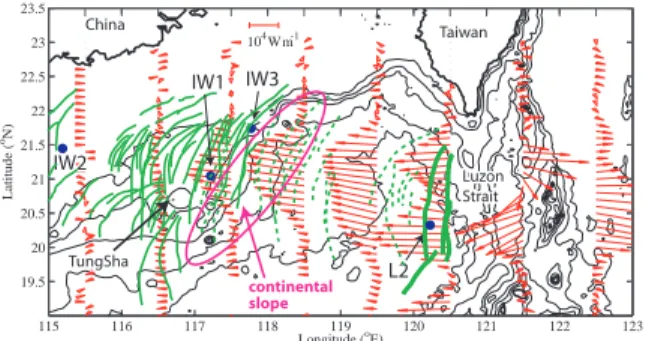
19.5 20 20.5 21 21.5 22 22.5 23 23.5 104 W m-1 Latitude ( oN) 115 116 117 118 119 120 121 122 123 Longitude (oE) Taiwan China L2 IW1 IW3 IW2 TungSha Luzon Strait continental slope
Figure 1. Map of South China Sea and positions of ADCP stations (blue dots). All ADCPs are RDI 150-kHz upward-looking, mounted on a buoy at 237-m depth at L2, IW1 and IW3, and on the bottom at IW2 (see also Fig. 2). Black contours are 200, 500, 1000, 2000, and 3000-m isobath. Red vectors are model results of depth-integrated semidiurnal internal tidal energy flux
produced by Niwa and Hibiya (2004). Green curves
are internal wave packets derived from SAR images by Zhao et al. (2004). Solid green curves indicate multiple-wave packets and dashed green curves single-multiple-wave pack-ets. Thick solid green curves west of Luzon Strait repre-sent the ”big wave” event observed in June 16 of 1995.
The generation mechanism for ISW in SCS is yet under debate. Two basic hypotheses have been proposed: 1)inter-nal soliton/lee wave model, and 2) nonlinear inter1)inter-nal tide model (Fig. 2)(Apel et al., 1997). In 1), lee waves are gen-erated between Batan Islands in Luzon Strait. When the current reverses, lee waves escape from the topography, de-velop into ISW (Fig. 2a) (Ebbesmeyer et al., 1991). In 2), internal tides could be generated either locally at the shelf break or remotely on two ridges in Luzon Strait (Fig. 1) (Niwa and Hibiya, 2004; Simmons et al., 2004). For the latter, they propagate across the SCS basin in a nearly-linear form. As internal tides amplified by shoaling conti-nental slope or front, they become nonlinear and evolve into ISW riding on internal tides (Fig. 2b). For ”very strong” barotropic tidal forcing in Luzon Strait, internal tides could be ”strongly” nonlinear near their generation sites where ISW evolve immediately (Fig. 2c).
Here, we analyze a set of four ADCP measurements taken simultaneously in different regions of the SCS. We will 1) de-scribe distinct internal wave characteristics, 2) discuss the generation mechanism of ISW, and 3) explore the relation between ISW in SCS and barotropic tidal forcing in Luzon Strait.
Observations
In April of 2000, three 150-kHz narrowband ADCP moor-ings (L2, IW1, and IW3) and one bottom ADCP (IW2) were
X - 2 LIEN ET AL.: INTERNAL SOLITARY WAVES IN SOUTH CHINA SEA deployed in SCS (Figs. 1 and 2) taking data for 20 days.
All ADCPs are upward-looking and record 1-min average data. The water depths at stations L2, IW1, IW3, and IW2 are 2080 m, 426 m, 468 m, and 110 m, respectively. The bin size is 10 m for L2, IW1, and IW3, and 5 m for IW2. The mooring ADCPs are mounted at a nominal depth of 237 m.
Internal Wave Characteristics
Internal waves in four locations within SCS show different characteristics. Segments of 4-hr time series for consecutive 6 semidiurnal periods are illustrated to show their differences (Fig. 3).
L2 mooring is located west of a submarine ridge in Luzon Strait. ADCP observations are available between 30 and 220-m depths. The zonal current u dominates the merid-ional current and is often >1 m/s. Strong tidal bores are observed. e.g, April 20 17:26-20:26. Here, the observed cur-rent is a combination of Kuroshio and tidal curcur-rents. Fol-lowing Pinkel (2000), we compute the stream function as
Ψ =R dz(u − C), where the wave speed C = 1.8ms−1 is
used (Yang et al., 2004; Chang, 2001). The zonal velocity between the sea surface and 30-m depth, missed by ADCP, is assumed constant and equals to u(30m). In other words, we have assumed a 2-D characteristics and a first-mode flow structure. Both assumptions might not be appropri-ate. Nevertheless, the computed stream line still provides a crude view of the isopycnal displacement. The zonal velocity and the streamline, starting at 100-m, show high-frequency variations riding on a low-frequency tidal displacement, but do not exhibit ISW (in contrast to those seen at IW1). This is the first in-situ evidence confirming the absence of ISW near Luzon Strait, except for one strong event (Hsu and Liu, 2000; Zhao et al., 2004). The vertical velocity at L2 is contaminated by the instrument noise and is not shown.
115 116 117 118 119 120 121 122 123 0 1000 2000 3000 4000 Longitude (oE) D e p t h ( m ) 0 1000 2000 3000 4000 D e p t h ( m ) 0 1000 2000 3000 4000 D e p t h ( m ) (a) (b) sho alin g Internal Soliton Model
Nonlinear Internal Tide Model
Luzon Strait Batan TungSha SCS R id g e R id g e T Weight Anchor Release ADCP 450 m 237 m IW1 (d) (d)
(c)Very Strong Nonlinear Internal Tide Model
IW1
IW2 IW3 L2
Figure 2. Sketch of generation mechanisms for ISW in SCS:(a) internal soliton model, (b) nonlinear internal tide model, and (c) very strong nonlinear internal tide model. The shading is the bathymetry across the South China Sea. The inset (d) shows the mooring ADCP con-figuration. Blue dots indicate locations of ADCP mea-surements.
At IW1, large ISW are observed at a semidiurnal period. The streamline follows the zonal shear very well, especially within the leading wave. All are depression waves. The leading waves have the vertical displacement of 70–120 m,
and a wave-width of 10-20 mins corresponding to 1–2 km in space. There are 2-5 trailing waves. More details of ISW at IW1 are described by Yang et al. (2004) and Chang (2001). These ISW have a 2-layer first-mode appearance. Before the arrival of waves, the current flows eastward. During the passage of waves, the zonal current in the upper layer fluctuates in alternating directions. The maximum west-ward current > 1ms−1 happens during the leading wave. The vertical velocity shows the most unambiguous first-mode depression wave structure, maximum vertical speed at mid-depth and strong downwelling followed by upwelling. The vertical speed of waves reaches to 0.2m/s. The quality of vertical velocity is confirmed by comparing observations with those predicted by the stream function. ISW at IW1 are the strongest among our observations, as also expected from SAR images and numerical model results of internal tides (Fig. 1). Z (m) Z (m) 0 50 100 150 200 04/18 15:50 0 60 120180 0 50 100 150 200 04/19 04:14 0 60 120180 04/19 16:38 0 60 120180 04/20 05:02 0 60 120180 04/20 17:26 0 60 120180 U (m /s ) -2 -1 0 1 04/21 05:50 W (m /s ) 0 60 120180 -0.2 -0.1 0 0.1 0.2 IW1 Z (m) 0 50 100 150 200 04/18 15:50 0 60 120180 04/19 04:14 0 60 120180 04/19 16:38 60 120180 04/20 05:02 0 60 120180 04/20 17:26 0 60 120180 U (m /s ) -2 -1 0 1 04/21 05:50 0 60 120180 mins L2 mins Z (m) Z (m) 0 50 100 150 200 04/18 11:10 0 60 120180 0 50 100 150 200 04/18 23:34 0 60 120180 04/19 11:58 0 60 120180 04/20 00:22 0 60 120180 04/20 12:46 0 60 120180 U (m /s ) -1 -0.5 0 0.5 1 04/21 01:10 W (m /s ) 0 60 120180 -0.1 -0.05 0 0.05 0.1 mins Z (m) 0 50 100 04/18 03:00 0 60 120180 0 50 100 04/18 15:24 0 60 120180 04/19 03:48 0 60 120180 04/19 16:12 0 60 120180 04/20 04:36 0 60 120180 U (m /s ) -0.5 0 0.5 04/20 17:00 W (m /s ) 0 60 120180 -0.1 -0.05 0 0.05 0.1 IW3 IW2 mins
Figure 3. The zonal velocity and vertical velocity con-tours in 4-hr time segments for 6 consecutive semidiurnal periods. Each segment is separated by a semidiurnal pe-riod 12.4 hr. The vertical velocity at L2 is not shown because it is contaminated by instrument noise. The be-ginning time for each time segment is shown below the labels of x-axis. The labels show minutes elapsed from the beginning time. The black curve shows the stream-line beginning at 100-m depth, assuming a westward wave speed of 1.8 m/s for L2, IW1 and IW3, and 0.8 m/s for IW2.
At IW3, only single depression waves are observed. The largest depression wave occurs at 0300 of April 21. The
LIEN ET AL.: INTERNAL SOLITARY WAVES IN SOUTH CHINA SEA X - 3
zonal velocity of the wave is 0.5 m/s, <1/2 of that in IW1. The mooring IW3 is located off shelf of ASIAEX (Ramp et al., 2003). Ramp et al. (2003) also report the absence of ISW at ASIAEX in 2000 and propose that a strong thermal front off the shelf prevents the penetration of ISW.
The IW2 is located on the continental shelf of 110-m
depth. Two trains of elevation waves are identified at 0300 of April 18 and 0548 of April 19. Here, a westward wave speed of 0.8 m/s is used which is determined by matching the observed vertical velocity with the prediction from the
stream function. The isopycnal displacement is generally
<10 m and the period is 20 minutes. The most distinct
characteristics for elevation waves is the leading upwelling followed by downwelling, best seen for the wave train at 0548 of April 19.
Internal Wave Spectra
Velocity Spectra are computed and WKB-normalized at each depths. Spectra are averaged over the upper 100 m and compared with the Garrett-Munk spectra (GM79) (Levine,
2002). The total energy spectrum (ΦE), horizontal velocity
spectrum (Φu), vertical velocity spectrum (Φw), and
po-tential energy spectrum (ΦP E) of GM79 are expressed as
follows, ΦE= Et N N0 B(ω) (1) Φw= Et (ω2− f2)N (N2− f2)N 0 B(ω) (2) Φu = 1 2 (N2− ω2)(ω2+ f2) (ω2− f2)ω2 Φw (3) ΦP E= 1 2 N2 ω2Φw, (4) where B(ω) = 2f
πω(ω2−f2)1/2. ω is frequency, N the
buoy-ancy frequency, and f the inertial frequency. Et = 2.9 mJ
kg−1 is the total energy per unit mass. N0= 0.0052 s−1 is
a reference Buoyancy frequency. We compute the potential energy spectrum using the observed vertical velocity spec-trum following eq (4).
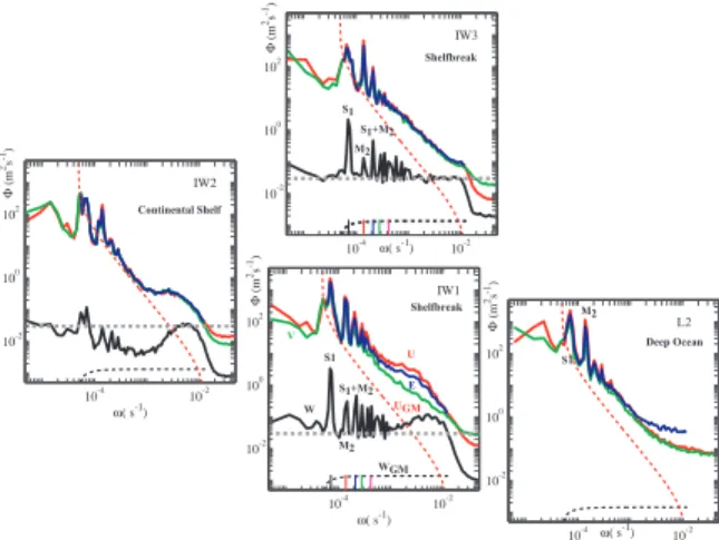
All horizontal velocity spectra show dominant diurnal and semidiurnal peaks, with differences in details. At L2, the two horizontal velocity spectra have a similar magnitude
and show a ω−2 spectral shape until they meet the noise
floor at about 0.003 s−1. The total internal wave energy
Eiw is 10 ×EGM, where EGM is the total energy of GM79
(Table 1).
At IW1, observed spectra exhibit peaks at diurnal, semid-iurnal, compound tides, and higher tidal harmonics suggest-ing nonlinear internal tides. Beyond tidal harmonics, 1) the
meridional velocity spectrum Φv shows an ω−2 shape
be-low N ( 0.016 s−1), 2) Φu shows a plateau of 5 ×Φv, and
3) Φw shows a broad bump in 0.001 s−1 < ω < N . The
total internal wave energy Eiw is 5.76 × 10⁻² m2s−2, 13
×EGM (Table 1). The vertical kinetic energy is 0.045 ×
10−2 m2s−2, 54 × the vertical energy of GM (W2
GM)! The
spectral plateau of Φu and the spectral bump of Φw
be-low N are associated with the ISW. The strong nonlinear tide and the accompanied enhanced ISW suggest their di-rect dynamic link, consistent with the internal tide model generation mechanism (Fig. 2b).
At IW3, spectral peaks exist at diurnal, semidiurnal, and compound tides, and higher tidal harmonic frequencies, sim-ilar to IW1 but of weaker magnitudes. Beyond the tidal har-monics, the two horizontal velocity spectra have the same spectral level with a spectral slope slightly greater than -2,
and Φwis white below N. The total internal wave energy, is
4 ×EGM, and the vertical energy is 25 ×WGM2 .
Fundamen-tal differences from IW1 are 1) the absence of the near-N
spectral bump of Φu and Φw at IW3, 2) the total internal
wave energy and vertical kinetic energy at IW3 is < 1/2 of those at IW1.
At IW2, all velocity spectra show peaks at the diurnal and semidiurnal frequencies, but not at higher tidal
har-monics. In 0.001 s−1< ω < N , all spectra exhibit a bump
10 times the background level. The near-N spectral bump is associated with the mixed elevation and depression ISW
(see Fig. 3). The total internal wave energy is 2 ×EGM,
and the vertical energy is 15 ×WGM2 .
10-4 10-2 10-2 100 102 L2 ω( s-1) Φ ( m 2s -1) 10-4 10-2 10-2 100 102 IW1 ω( s-1) Φ ( m 2s -1) 10-4 10-2 10-2 100 102 IW2 ω( s-1) Φ ( m 2s -1) 10-4 10-2 10-2 100 102 IW3 ω( s-1) Φ ( m 2s -1) S1 S1 S1 M2 M2 M2 S1+M2 S1+M2 W U V E WGM UGM Continental Shelf Shelfbreak Shelfbreak Deep Ocean
Figure 4. Average velocity and energy spectra. Spec-tra are WKB-normalized and averaged over the upper 100m. Panels are arranged roughly following the loca-tions of ADCP staloca-tions. Red, green, and black curves represent zonal, meridional and vertical velocity spectra, respectively. Blue curves are total energy spectra. Black and red dashed curves are GM79 vertical and horizon-tal velocity spectra. The thick dashed gray lines are the observed vertical velocity spectrum at IW3 averaged in 0.001 < ω < N , plotted for reference. Frequencies of di-urnal tide, S1, semididi-urnal tide, M 2, and the compound tide, M 2 + S1 are labeled.
The presence of strong ISW at IW1 and its absence at L2 shown in time series and spectral properties suggest that ISW in SCS are generated via the nonlinear internal tide model (Fig. 2b), instead of the lee wave model (Fig. 2a).
Energy of ISW and Tidal Forcing
Internal solitary waves contain more than 80% of the ver-tical energy in the internal wave band (Table 1). There-fore, the vertical energy is an ideal index for the energy of ISW. The vertical velocity variances, computed in 1-hr in-terval, at IW1 show a semidiurnal periodicity (Fig. 5b). The barotropic tidal height in Luzon Strait, computed us-ing Oregon Tidal Inversion Software (OTIS) (Egbert and Erofeeva, 2002) is also dominated by the semidiurnal tide (Fig. 5a). Both variables show a fortnightly modulation and are correlated with a phase lag of 1.85 day lead by the tide (Fig. 5c). Niwa and Hibiya (2004) show that the M2
energy flux is mostly emanated from the western submarine ridge, 300–350 km from IW1. Considering the 1.85-days phase lag as the travel time, the speed of the semidiurnal
X - 4 LIEN ET AL.: INTERNAL SOLITARY WAVES IN SOUTH CHINA SEA
internal tide should be 1.88–2.20 m s−1, a reasonable
esti-mate. The correlation between the rms tidal amplitude in
Luzon Strait (σH) and the rms vertical velocity at IW1 (σw)
is 0.89 with the 95% significance level of 0.3 . An orthogonal linear regression fit (Fig. 5d) yields
σw(m/s) = 0.11σH(m) − 0.01(m/s) (5)
This relation provides a simple prediction of ISW near Tung-Sha Island with the barotropic tide at Luzon Strait. The
correlation increases to 0.96 if the linear trend of σw is
re-moved. -1 0 1 Tide (m) 0 0.005 0.01 σw 2 (m 2s -2) 0.02 0.04 0.06 0.2 0.4 0.6 σw (m s -1) Apr 10 15 20 25 30 May 5 Year 2000 σH (m) Luzon Strait (a) (b) (c) 0.2 0.4 0.6 0.02 0.04 0.06 σH (m) σw (m /s ) (d)
Figure 5. Time series of (a) the barotropic tide east of Luzon Strait HLS(123
◦
E, 21◦N) (black curve) and the rms tidal amplitude computed in 24-hr interval σHLS(red curve), (b) the vertical velocity variance computed in 1-hr interval σw2 (black curve), and the 1.85-day forward
shifted HLS (red curve), (c) the rms vertical velocity σw
(gray curve) computed in 24-hr interval and the 1.85-day forward shifted σHLS (red curve). The blue curve in (c) is the detrended σw. The inset (d) shows the scatter plot
between 1.85-day shifted σHLS and σw (red dots), and between 1.85-day shifted σHLS and detrended σw (blue dots). The black line represents the orthogonal regression fit.
Discussions
Generation Mechanisms
Results of the present analysis suggest that ISW in SCS are primarily evolved from nonlinear internal tides because 1)ISW are not observed near Luzon Strait and 2) strong ISW are observed at IW1 mooring with accompanied non-linear internal tides. ISW could also be generated at the local shelf break, e.g., on the Oregon shelf (Moum et al., 2003). Within the internal tidal beam emanated from the Luzon Strait, e.g., IW1, ISW evolve primarily from the am-plification of the trans-basin internal tides. Outside of the internal tidal beam, e.g., IW3, ISW may evolve from the locally generated internal tides.
Big Wave near Luzon Strait
A long-crest ISW was captured by the satellite image on June 16 of 1995 (Hus and Liu, 2000). It happened when the barotropic tidal current in Luzon Strait, computed us-ing OTIS, was one of the strongest of 1995 (Fig. 6). We propose that the ”big wave” west of Luzon Strait is gener-ated by an abnormally strong barotropic tidal forcing. These events occur only a few days a year. The chance for satellite
images to capture these events is slim, one capture in nearly 10 years of satellite images.
Feb 16 Apr 16 Jun 16 Aug 16 Oct 16 Dec 16 -1 -0.5 0 0.5 1 1.5 2 U BT (m/s) Year 1995
Figure 6. Barotropic zonal tidal current in Luzon Strait in 1995 produced by OTIS (Egbert and Erofeeva, 2002).
Energy Conversion from Internal Tides to ISW At IW1, the total energy of ISW is found to be 92 ×10−4 m2 s−2(Table 1), 16% of the total internal wave energy. In
other words, the energy conversion rate from internal tides to ISW is 16%. Niwa and Hibiya (2004) found 4.2 GW M2
internal tidal energy flux into SCS, mostly in a 100-km-wide tidal beam colliding onto the continental slope (Fig. 1). Assuming a 16% conversion rate, ISW should contain 0.67 GW of energy flux. If all ISW dissipate within the 200 km x 200 km area centering at TungSha Island, the depth-integrated dissipation rate is 1.7 ×10⁻⁵ W m kg−1. If we further assume that most of turbulence dissipation occur at the O(10m)-thick interface, as found by Moum et al. (2004), the turbulence kinetic energy dissipation rate ε associated with ISW near TungSha Island would be O(10−6W kg−1) and an eddy diffusivity Kρ= 0.2εN−2= O(10−3) m2 s−1.
Prediction of Internal Solitary Waves in SCS
The energy content of ISW depends on 1) the energy conversion rate from the barotropic to internal tides, 2)from internal tides to ISW, 3) the internal tidal beam properties, and 4) the propagation and dissipation of ISW. These pro-cesses are modulated by the barotropic tides, by the back-ground shear and stratification associated with Kuroshio,
Table 1. Summary of vertical kinetic energy in the internal
wave band (W2
iw) averaged in the upper 100 m, total internal
wave energy (Eiw ), the ratio of the observed vertical energy
W2
iwto the GM79 vertical kinetic energy (WGM2 ), the ratio of
Eiw to GM total energy (EGM ), the vertical kinetic energy
in the high-frequency regime (10−3s−1< ω < N ) W2
isw, the
total energy in the high-frequency regime Eisw, the
percent-age of W2
iswin Wiw2 (%Wisw2 ), and the percentage of Eisw in
Eiw(%Eisw). Stn W2 iw Eiw Wiw2 W2 GM Eiw EGM W 2
isw Eisw %Wisw2 %Eisw
(cm2 s2 ) ( cm2 s2 ) ( cm2 s2 ) ( cm2 s2 ) (%) (%) L2 NA 546 NA 10.2 NA NA NA 10 IW1 4.5 576 53.5 12.9 4 92 89 16 IW3 2.1 243 24.8 4.3 1.7 26 81 11 IW2 1.3 140 14.7 2.4 1.2 20 93 14
LIEN ET AL.: INTERNAL SOLITARY WAVES IN SOUTH CHINA SEA X - 5
mesoscale eddies, and by the surface wind and buoyancy forcing in the entire SCS including Luzon Strait. The simple relation (5) includes only one of many important parame-ters, implying an invariant conversion rates from barotropic to internal tides, and from internal tides to ISW. The fair success of this simple relation comes from 1) that other pa-rameters are nearly invariant in a monthly time scale, and 2) that, at IW1, internal tides generated remotely in Luzon Strait dominates that generated locally. The linear trend of
σw(Fig. 5c) represents effects of processes expressed in (5).
Summary
Distinct low-frequency and high-frequency internal wave properties are revealed at four different locations in SCS. At the path of the model internal tidal beam west of continental slope, the internal wave energy is 13 times GM, the vertical energy is 54 times GM, the tides are nonlinear, and ISW of O(100m) amplitude are observed repeatedly. These results suggest ISW are primarily caused by the nonlinear inter-nal tides amplified near the continental slope on their beam path. Large-amplitude ISW are not observed near Luzon Strait suggesting that ISW are not escaping lee waves. The ”big wave” near Luzon Strait observed on June 16 1995 is a rare even, resulted from an abnormally strong barotropic tidal forcing.
The rms vertical velocity observed near TungSha Island is linearly proportional to the barotropic tide in Luzon Strait. This provides a zeroth order prediction of ISW energy in SCS. A more accurate prediction should include processes describing energy conversion among barotropic tides, inter-nal tides, and interinter-nal solitary waves, interinter-nal tidal beam structure and propagation properties, and dissipation of ISW. Further observations and numerical models are needed to improve our understanding of the details of these pro-cesses, and implement into the prediction of ISW.
Acknowledgments. We would like to thank Drs Yoshihiro Niwa and Toshiyuki Hibiya for providing their model results of internal tidal energy flux in South China Sea. Discussions with Drs. Wen-Ssn Chuang, Mathew Alford, and Zhongxiang Zhao are very helpful. This work is supported by Office of Naval Research.
References
Apel, J. R., M. Badiey, C.-S. Chiu, S. Finette, R. Headrick, J. Kemp, J. F. Lynch, A. Newhall, M. H. Orr, B. H. Pase-wark, D. Tielbuerger, A. turgut, K. von der Heydt, and S.
Wolf (1997), ”An overview of the 1995 SWARM Shallow-Water Internal Wave Acoustic Scattering Experiment”, IEEE
J. Oceanic Eng., , 22, 465–500.
Chang, M.-H. (2001), A study of internal solitons in the South China Sea, M. S. thesis, National Taiwan University, Taiwan, 31pp.
Egbert, G. D. and Erofeeva, S. Y. (2002). Efficient inverse mod-eling of barotropic ocean tides. J. Atm. and Ocean. Tech., 19, 183–204.
Ebbesmeyer, C. C., C. A. Coomes, and R. C. Hamiloton, K. A. Kurus, T. C. Cullivan, B. L. Salem, R. D. Romea, and R. K. Bauer (1991), New observations on internal waves (soliton) in the South China Sea using an acoustic Doppler current pro-filer, Marine Tech. Soc. 91 Proc., New Orleans, pp. 165–175. Hsu, m.-K., and A. K. Liu (2000), Nonlinear internal waves in
the South China Sea, Can. J. Rem. Sens., 26, 72–81. Levine, M. (2002), A modification of the Garrett-Munk internal
wave spectrum, J. Phys. Oceanogr., 32, 3166–3181.
Moum, J. N., D. M. Farmer, W. D. Smyth, L. Armi, and S. Va-gle (2003), Structure and generation of turbulence at interfaces strained by internal solitary waves propagating shoreward over the continental shelf, 33, 2093–2112.
Orr, M. H., and P. C. Mignerey (2003), Nonlinear internal waves in the South China Sea: OBservation of the conversion of de-pression internal waves to elevation internal waves, J. G. R.,
108, C3, doi:10,.1029/2001JC00163.
Pinkel, R. (2000), Internal solitary waves in the warm pool of the western equatorial Pacific, J. Phys. Oceanogr., 30, 2906–2926. Ramp., S. R., J. F. Lynch, P. H. Dahl, C.-S. Chiu, J. A. Simmen (2003), Program foster advances in shallow-water acoustics in Southeastern Asia, EOS, 884, 37, 361–376.
Ramp, S. R., D. Tang, T. F. Duda, J. F. Lynch, A. K. Liu, C.-S. Chiu, F. Bahr, H.-R. Kim, and Y. J. Yang (2004), Internal solitons in the northeastern South China Sea Part I:Sources and Deep Water Propagation, IEEE J. Ocean Eng., in press. Simmons, H. L., R. W. Hallberg, and B. K. Arbic (2004), Inter-nal wave generation in a global baroclinic tide model, Deep-Sea
Res., in press.
Yang, Y. J., T. Y. Tang, M. H. Chuang, A. K. Liu, M.-K. Hsu, and S. R. Ramp (2004), Solitons northeast of TungSha Island during the ASIAEX pilot studies, IEEE J. Ocean. Eng., Spe-cial Issue on Asian Marginal Seas, in press.
Zhao, Z., V. Klemas, Q. Zheng, and X.-H. Yan (2004), Remote sensing evidence for baroclinic tide origin of internal solitary waves in the northeastern South China Sea, Geophys. Res.
Let., 31, doi:10.1029/2003GL019077.
R.-C. Lien, Applied Physics Lab, University of Washington, Seattle, WA 98105, USA. ([email protected])
Intra-seasonal variation in the velocity field of the
northeastern South China Sea
Chau-Ron Wu1, T. Y. Tang2,*, S. F. Lin2,3, Y. J. Yang4, and W.-D. Liang4
1
Department of Earth Sciences, National Taiwan Normal University, Taipei, Taiwan, ROC
2
Institute of Oceanography, National Taiwan University, Taipei, Taiwan, ROC
3
Energy & Resources Laboratories, Industrial Technology Research Institute, Hsinchu,
Taiwan, ROC
4
Department of Marine Science, Chinese Naval Academy, Kaohsiung, Taiwan, ROC
*
Corresponding author. Institute of Oceanography, National Taiwan University, P.O. Box 23-13, Taipei, 106, Taiwan, ROC, Tel: +886-2-23626097; Fax: +886-2-23698526; Email
address: [email protected]
Submitted to
Geophysical Research Letters
1
Abstract
Two subsurface Acoustic Doppler Current Profilers (ADCP) were deployed at the northeastern South China Sea to study circulation structure in the area as well as the path
and process of Kuroshio intrusion. The 48-hour low-pass filtered data reveal significant intra-seasonal variations in the velocity field. The current pattern alternates between
clockwise and counterclockwise even within a single month. Local wind forcing
dominated by monsoon winds fails to address the phenomena and variations. The present
study suggests that wind stress curl forcing is the dominant process controlling the
circulation picture in the area. While a stronger wind stress curl appeared and developed off southern tip of Taiwan, it will provide negative vorticity to the intruded current and
form an anticyclonic eddy. The stronger current is always going along with the stronger wind stress curl. On the other hand, while the curl in the area looses or decays, the
intruded current becomes weakened and forms a cyclonic eddy. The agreement between wind stress curl and the velocity field suggests that changes in the wind stress curl
2
Introduction
The circulation structure in the northeastern South China Sea is extremely
complicated. In addition to the location with a complicated topography and seasonal reversal monsoon, the regions might be interacted between currents from both northern
South China Sea and Taiwan Strait. Furthermore, it is well known that the Kruoshio front might reach the sea southwest of Taiwan and influence the shelf break circulation [Fan
and Yu, 1981]. All of these factors induce varieties of contributions and alter the current
structures in the regions. Especially the intrusion current from Kuroshio front, it might be
the most important component and be the major theme in the area.
The Pacific western boundary current, the Kuroshio, flows northward and bypasses east of Luzon and Taiwan [Nitani, 1972]. Similar to the Loop Current in the Gulf of
Mexico, the Kuroshio water has also been reported to intrude the Luzon Strait where
plays a deep gap in the western boundary [Nitani, 1972; Shaw, 1991]. Since the Luzon Strait is the only deep passage of the South China Sea, the intrusion of water from
Kuroshio is important to the salt budget in the basin. Seasonal variations of Kuroshio intrusion have been reported extensively in a wealth of existing literature [e. g. Wyrtki,
3
challenged by several recent observations. For example, both moored current data and
ship-board ADCP data evidenced that the westward trend of Kuroshio intrusion is persisted all the year round [Liang et al., 2003; Tang et al., 2003].
Furthermore, although the intrusion of waters from the Kuroshio to the northeastern South China Sea has been studied for several decades, the path and process of Kuroshio
intrusion in the region remained discrepancies among oceanographers. For example, based on hydrographic data, Wang and Chern [1987] inferred an anticyclonic (clockwise)
eddy occupied the area at the onset of the northeast monsoon. Also based on
hydrographic data in May and August 1986, on the other hand, Shaw [1989] suggested that the intrusion current was probably part of a cyclonic (counterclockwise) circulation
in the northern South China Sea. Anticyclonic or cyclonic circulation is of importance to the distribution of the water masses in the region. A correct description of circulation
pattern is essential to future dynamic studies of the intrusion process.
In this study, current and hydrographic data from two mooring stations were
examined to study the circulation pattern in the region. The direct observations in the velocity field are capable of determining the distribution of the Kuroshio intrusion water
and inferring the path of intrusion. The results show that significant intra-seasonal
4
counterclockwise. Wind stress curls were also calculated from the blended QSCAT/NCEP
(NASA Quick Scatterometer/National Centers for Environmental Prediction) wind stress fields at a resolution of 0.5° x 0.5° [Milliff et al., 1999] to examine the driving mechanism
of the local current.
Mooring data
Two sets of subsurface moorings (named St. W and St. E) were deployed in the west and east of the shelf break northeast of the South China Sea, respectively. Figure 1 shows
the mooring locations and the surrounding bathymetry. Each set of mooring includes an
upward-looking, 150 kHz, self-contained Acoustic Doppler Current Profiler (ADCP) mounted on a 45” diameter spherical syntactic foam buoy and a SEACAT
Conductivity-Temperature-Depth (CTD) mounted 5 m beneath the ADCP. The water depths at St. W and St. E are 1014 m and 968 m, respectively. Table 1 lists the locations
and local water depths for each mooring, the depths of instruments, the duration of deployments, and the vertical range of current profile measured by the ADCP. The bin
length of ADCP was set as 8 m. The hourly current velocity was recorded averaged over 240 pings for board-band ADCP. The standard deviations of measurement velocity were
1.2 cm s-1. The obtained current velocity of ADCP was corrected for vertical excursion
5
deviation. Finally, the vertical profile of current velocity was linearly interpolated and
resampled at 10 m intervals. The time series of current velocity discussed in the following sections were low-pass filtered to remove the fluctuations for frequencies higher than 0.5
cycles per day.
Results and discussion
Low-pass filtered velocity
Figure 2 shows the eastward (U) and northward (V) components of 48-hour
low-pass filtered current velocity at St. W. In general U component is stronger than V
component and the currents decrease but keep the direction with depth. Both U and V components show significant intra-seasonal variations. By November 2000, U component
is weak and alternates directions between westward and eastward. The current enhances and turns eastward in December, reaching its maximum strength in the end of December.
Just in the beginning of January, the eastward current decreases suddenly and reverses thereafter. Until March 2001, a repeat behavior takes place when eastward flow appears
in the middle of March and reaches its maximum in the end of the month, turning
westward suddenly afterward. Similar pattern but leading around half month is presented
in the V component. In the beginning of both December 2000 and March 2001, the V
6
Similar to Figure 2, Figure 3 shows U and V components of low-pass filtered
velocity at location St. E. Significant intra-seasonal variations are also evidenced at St. E. Graphically, U component is generally weak except in October, November 2000 and
February 2001 when stronger currents with speed more than 50 cm s-1 occur and all of
them flow eastward. Two periods of weak westward currents present in January and
middle March 2001. Frequently reversal currents are shown in v component. Prior to middle of December, currents flow southward mostly, turning northward thereafter.
Stronger southward currents show again in the middle of February, reaching its maximum
speed of 100 cm s-1 on March 1, 2001. The current turns northward in the middle of
March and persists into April. Furthermore, the intra-seasonal variation at St. E seems to
agree well with that at St. W, indicating that St. E and St. W are related to each other somehow. To emphasize this, the stick plots of depth average at St. W (20-130 m) and St.
E (20-180 m) are shown together in Figure 4. Similar intra-seasonal reversals of currents between St. W and St. E come to the first sight. However, it seems that changes in St. E
generally lead those in St. W around 10~15 days. The phenomenon deserves to further verify and will be examined in detail later in this section.
In Figure 4, northward flow prevails at St. W and southeastward flow exists at St. E
7
a conceptual clockwise circulation pattern. Currents at St. W reverse southwestward and
meanwhile currents at St. E turn either northwestward or northeastward during the period from middle December to middle February. The reversal phenomena suggest that current
pattern alters from clockwise circulation to counterclockwise in the study region.
Clockwise circulation dominates again during the period from middle February to middle
March. Note that the currents are always stronger during clockwise circulation. After March, weak counterclockwise circulation plays the finale. Furthermore, as mentioned in
the introduction section, currents perform an anticyclone or a cyclone might directly
influence the geographic distribution of the water masses in the region. Without a correct description of circulation pattern, it is not possible to identify the water masses and to
verify the intrusion process.
Water masses and circulation pattern
To describe the distribution of various water masses and the path of Kuroshio intrusion, the mooring CTD data at both St. W and St. E were plotted in Figure 5. Also
join with velocity vectors to separate different episodes of clockwise and
counterclockwise circulation. In the figure, the red color represents circulation pattern is
clockwise while the blue represents there is counterclockwise circulation. Temperature
8
respectively. Although the absolute values of CTD data are probably problematic, the
relative value can still be applied to identify where the water masses come from. Since not only temperature but salinity of St. E are generally lower than those of St. W, the
measured depth at St. E is deeper could not account for the phenomena singly. Rather, there must be colder and fresher water entering and mixing with the local water around
regions of St. E. Based on long-term mooring observations around sea southwest of Taiwan, mean current always flows southeastward during winter [Chern, 1982]. With
mixing cold and fresh coastal water from Taiwan Strait, it makes sense that temperature
and salinity at St. E should be lower than those at St. W.
Furthermore, concerning the temporal variability in each station, both stations show
that temperature is higher whenever clockwise circulation dominates in the region. The temperature difference is more distinct at St. W where is far away from influence of
colder coastal water (Figure 5). The higher values of temperature were presented during two periods in December 2000 and in March 2001. The results are reasonable and can be
explained by water movement. Currents generally intensify while clockwise circulation performs as mentioned earlier so that stronger intrusion current brings in warmer water
from Kuroshio front and then increases water temperature at St. W. On the other hand,
9
weak and flows westward continuously along its northern boundary in Taiwan Strait. By
gradually mixing with cold front from Taiwan Strait, the water temperature decreases. To further study alternation of circulation pattern and relation between St. W and St.
E, we rotated the current velocity to its principal axis. The principal axis of St. W is 45° clockwise-rotated Cartesian (northeastern-southwestern) and St. E is 135°
clockwise-rotated Cartesian (southeastern-northwestern). Figures 6a and 6b show time series of principal axis depth-average current velocity at St. W and St. E, respectively.
Graphically, both St. W and St. E evidence two significant peaks. However, the timing is
not consistent with each other. Two peaks at St. W are during the periods December and March while at St. E are from middle November to middle December and from middle
February to middle March. The results demonstrate that St. E leads St. W and an interval of 315-hour might properly describe time lag of St. W. In Figure 6c, St. E with time lag
of 315 hours is overlapped to St. W. Peak-to peak comparison indicates that the variations of St. W and those in time lag of St. E are frequently in phase, suggesting St. E leads St.
W by 10~15 days indeed. The trend is always valid whatever during episode of clockwise or counterclockwise circulation. The fact that St. E leads St. W during clockwise episode
is probably against intuitive. Therefore, not merely a single anticyclone structure might
10
Mechanism
What causes the intra-seasonal variation in the area deserves to further investigate. Intuitively, currents in the area, especially those near surface currents, should be driven
by the strong monsoon during winter when northeasterly winds prevail. However, there is almost no correlation between the current and local wind forcing from weather station at
Tung-Chi Island (figure not shown). Based on model simulations in the South China Sea,
Wu et al. [1998] suggested that the formation of a gyre, whatever anticyclonic or cyclonic,
is essential determined by the wind stress curl. Shaw et al. [1999] also found that the first
two empirical orthogonal functions (EOF) modes of the wind stress curl agree well with those in the corresponding altimeter sea level modes, further supporting the wind stress
curl forcing scenario. However, it is not clear whether the wind stress curl is also
important to meso-scale circulation as in the present study. Since the scale is quite small
in the present study, high-resolution winds are indeed in need. We adopted 6-hourly maps of 10 m zonal and meridional wind components at a resolution of 0.5° x 0.5°, which is
derived from a space and time blend of QSCAT-DIRTH satellite scatterometer
observations and NCEP analyses [Milliff et al., 1999]. The blended data set is one of the
11
In this section, wind stress curls are calculated from the blended wind stress fields.
Figure 7 shows the monthly mean of the wind stress curl during the six-month period. The days in February and March 2001 have been slightly adjusted to fit the intra-seasonal
variation in the velocity field. Main features in the intra-seasonal variation of the wind stress curl are captured in the sequence of plots from (a)-(f). In October 1999 (Figure 7a),
a dipole structure with positive value to the north appeared in the region. Note that the south portion is what we should be more concern about since its position approaches the
Kuroshio intrusion. Off southern tip of Taiwan, the large and negative curl extends
southwestward in October that marks the onset of the winter monsoon. The pattern persists well into November, gradually increasing its strength in December. In the
following month, the southern curl weakens (Figure 7d). The curl increases again and reaches its maximum strength during the period from February 10 to March 10 (Figure 7e)
and decays afterwards (Figure 7f). The variations of the southern curl are corresponding to those shown in the velocity field and the curl is capable of explaining the
intra-seasonal variations in the velocity field. While the southern curl appeared and developed in the position, the intruded current from Kuroshio would form anticyclonic
eddies clockwise because the curl provides negative vorticities to the current. Note that
12
stronger anticyclone might occur in close vicinity of St. E merely. The loosed clockwise
vortexes might shed away from St. E while the corresponding Reynolds number is large enough. The large value of curl also explains the reason why the current is accelerated
during clockwise circulation dominated episode as mentioned earlier. For example, the
strongest southward current at St. E with maximum speed of 100 cm s-1 shown on March
1, 2001 is well corresponding to the strongest southern curl in Figure 7e. On the other hand, while the southern curl weakens or looses (Figure 7d, 7f), the intruded current
overwhelms the curl and continues westward along the shelf break, forming a weak
cyclonic (counterclockwise) eddy. Weaker currents in these two counterclockwise episodes are also noted in the previous section.
Summary and Conclusions
Although the East Asian monsoons dominate, an intra-seasonal instead of seasonal
variation in the velocity field has been found in the region. The agreement between wind stress curl and velocity fields suggests that the wind stress curl could be the main driving
force to trigger the intra-seasonal variations. The intensity of wind stress curl off southern tip of Taiwan could determine whether clockwise or counterclockwise circulation pattern
performs in the region. While the southern curl enhanced, the intruded current strengthens
13
mooring velocity data indeed evidence that currents during clockwise circulation are
much stronger than those during counterclockwise. Temperature is also higher while clockwise since the stronger intrusion current will bring in Kuroshio warmer water and
increase local water temperature. Acknowledgements
We would like to thank Mr. Y. C. Tsai for processing the mooring data. This research was supported by the National Science Council, Taiwan, ROC, under grants NSC
89-2611-M-002-031-OP2 (TYT), NSC 91-2611-M-003-004 (CRW), and NSC
14
References
Chern, C. S., Current and wave measurement in the vicinity of Hsien-Da-Kang and Tung- Kang (continued), Special Pub. 39, Inst. of Oceanogr., Natl. Taiwan Univ., Taiwan,
1982.
Fan, K. -L., and C.-Y. Yu, A study of water masses in the seas of south most Taiwan, Acta
Oceanogr. Taiwan., 12, 94-111, 1981.
Liang, W.-D., T. Y. Tang, Y. J. Yang, M. T. Ko, and W.-S. Chuang, Upper-ocean current
around Taiwan, Deep-Sea Res. II, 50, 1085-1105, 2003.
Milliff, R. F., W.G. Large, J. Morzel, G. Danabasoglu, and T. M. Chin, Ocean general circulation model sensitivity to forcing from scatterometer winds, J. Geophys.
Res., 104, 11337-11358, 1999.
Nitani H., Beginning of the Kuroshio, in Kuroshio, pp. 129-163, Univ. of Wash. Press,
Seattle, Wash., 1972.
Shaw, P.-T., The intrusion of water masses into the sea southwest of Taiwan, J. Geophys.
Res., 94, 18213-18226, 1989.
Shaw, P.-T., S.-Y. Chao, and L.-L. Fu, Sea surface height variations in the South China
Sea from satellite altimetry, Oceanol. Acta, 22, 1-17, 1999.
15
Strait, J. Phys. Oceanogr., submitted, 2003.
Wu, C.-R., P.-T. Shaw, and S.-Y. Chao, Seasonal and interannual variations in the velocity field of the South China Sea, J. Oceanogr., 54, 361-372, 1998.
Wang, J. and C. S. Chern, The warm-core eddy in the northern South China Sea, Preliminary observations on the warm-core eddy, Acta Oceanogr. Taiwan., 18,
92-103, 1987.
Wyrtki, K., Physical oceanography of the southeast Asian waters, Scientific Results of
Marine Investigation of the South China Sea and the Gulf of Thailand, NAGA
Report Vol. 2, 195 pp., Scripps Institution of Oceanography, La Jolla, California,
16
TABLE 1. Mooring locations; water, ADCP and CTD depths; durations; and data
distribution depths (interval of 10 m) at St. W and St. E, respectively.
Station Longitude Latitude Water
Depth ADCP Depth CTD Depth Duration Measurement Range St. W 118° 44’E 22°N 1014 m 160 m 165 m 2000/10/13~ 2001/04/18 20~130 m St. E 120° 10’E 22°N 968 m 202 m 207 m 2000/10/04~ 2001/04/18 20~180 m
17
Figure Captions
Figure 1. The study area with locations of mooring stations (squares) and Tung-Chi Island (asterisk). The current distribution at 30 m is adopted from Liang et al. [2003].
Figure 2. Vertical sections of 48-hr low-pass current velocity observed at St. W. Contour
interval is 10 cm s-1.
Figure 3. Same as Figure 2 except at St. E.
Figure 4. Stick plots of the depth-averaged current velocity at St. W and St. E,
respectively.
Figure 5. T-S diagram at St. W and St. E. Velocity vectors are also presented to separate different episodes of clockwise (red) and counterclockwise (blue) circulation.
Figure 6. Time series of principal axis depth-average current velocity at St. W and St. E, respectively. St. E with time lag of 315 hours is overlapped to St. W shown in
the bottom panel as well.
Figure 7. Monthly mean of the wind stress curl during the six-month period. Contour
-8000 -7000 -6000 -5000 -4000 -3000 -2000 -1000 0 m 116˚E 116˚E 118˚E 118˚E 120˚E 120˚E 122˚E 122˚E 18˚N 18˚N 20˚N 20˚N 22˚N 22˚N 24˚N 24˚N 100 cm/sec
W
E
South China Sea
116˚E 116˚E 118˚E 118˚E 120˚E 120˚E 122˚E 122˚E 18˚N 18˚N 20˚N 20˚N 22˚N 22˚N 24˚N 24˚N
Taiwan
Luzon
China
116˚E 116˚E 118˚E 118˚E 120˚E 120˚E 122˚E 122˚E 18˚N 18˚N 20˚N 20˚N 22˚N 22˚N 24˚N 24˚N-0.1 0 0 0 0.1 0.2 0 0 0
118˚E 119˚E 120˚E 121˚E 122˚E
20˚N 21˚N 22˚N 23˚N 24˚N Oct. 10~31 2000 -0.2 -0.1 0 0 0.1 0.1 0 0 20˚N 21˚N 22˚N 23˚N 24˚N Nov. 1~30 2000 -0.2 -0.1 -0.1 0 0.1 0
118˚E 119˚E 120˚E 121˚E 122˚E
20˚N 21˚N 22˚N 23˚N 24˚N Dec. 1~31 2000 -0.1 0 0.1 0
118˚E 119˚E 120˚E 121˚E 122˚E
20˚N 21˚N 22˚N 23˚N 24˚N Jan. 1~31 2001 -0.2 -0.1 -0.1 0 0.1 0 20˚N 21˚N 22˚N 23˚N 24˚N Feb. 10~ Mar. 10 2001 0 0 0 0
118˚E 119˚E 120˚E 121˚E 122˚E
20˚N 21˚N 22˚N 23˚N 24˚N Apr. 1~20 2001
5. Summary
The proposed work has been done. The collected data show a number of interesting features. The future work will be primarily to study those features. The study will include not only the present data it also will include the previous data. An integrated investigate is required. Except the academic study, the work in the next fiscal year will be the mooring refurbishment and exchange ideas among the domestic PIs as well as the foreign PIs.