Automatic Segmentation of Brain MRI Images by Threshold Level Set Method

全文

(1)Automatic Segmentation of Brain MRI Images by Threshold Level Set Method Chih-Yu Hsu1＊., Chih-Hung Yang 2, Lin-huang Chang 3, Zsu- Uei Zchang 4 Department of Medical Imaging and Radiological Sciences, Chung Shan Medical University,Taiwan 2 Department of Applied Mathematics, National Chung-Hsing University, Taichung, Taiwan 1. Institute of Networking and Communication Engineering, ChaoYang University of Technology,Taiwan 4 Institute of Biomedical Engineering, National Taiwan University,Taiwan [email protected], [email protected], [email protected], [email protected] 3. ＊. Corresponding author, e-mail: [email protected].. Abstract A threshold level set method with adaptive parameters applied on automatic segmentation of brain MRI image is presented in this paper. Threshold level set method is one kind of the active contour models applied on the image segmentation. There are two parameters of threshold level set for adjusting threshold purposes. These two thresholds adjust the speed function for controlling the stop position of the contours. The optimal parameters are automatically decided by using the adaptive parameter selection algorithm. The contours of brain white matter are segmented with MRI images by both the developed method and manual operation. By experiment results, it is demonstrated that the proposed method is effective and efficient than manual selection of parameters. Keywords: MRI Images, Image Segmentation, Level Set Method, Active Contour Model. 1. Introduction. Segmentation is a technology to extract the interested features form images and it is a necessary operation on medical image to find shapes of tissues. The tissues of human body mostly are deformable and it’s suitable to using deformable models analysis the structure of tissue. The deformable models describe the deformation of elastic structures under external loads and constraints. Since 1986, Terzopoulos apply deformable models on image matching computer vision and computer graphics [1-5]. Segmentation method can be classified by obtaining regions of pixels or contour pixels of objects. The Active Contour Model (ACM) belongs to the later. It first is proposed by Kass, Witkin and Terzopoulos [1] in 1988 and is popularly known as” Snake”. It can capture the contour of objects in image [5] and is wieldy used and discussed. They are sometimes called as the classical active contour models [1]. The GVF active contour model [10] modified the image force to conquer the drawbacks of classical active contour models. This is. the most concepts of active contour models with an edge-detector is used, depending on the gradient of the image, to stop the evolving curve on the boundary of the desired object. Some related works ([19], [20], and [22]) discuss the successes and problems with implementation active contours on segmentation. Energy method combined with variation calculus, Minimum potential principle and Hamiltonian theory are well applied on Elasticity and Dynamical Structure Analysis. The Active Contour Model introduces the same variation framework to solve segmentation problem. Minimum potential principle or Hamiltonian theory combined with the variation calculus technique is to minimization a functional to obtain the governing equations called as Euler-Lagrange equations. These solutions of these equations are desired curves. There are two kinds of functional, Mumford–Shah functional and Functional used by Kass-Witkin-Terzopoulos model, famous. Active contours described by Euler-Lagrange equations can be classified as two kinds of curves according to their mathematic descriptions. One is parametric curves and the other is geometric curves. Parametric active contours are explicitly represented as parameterized curves. They are called as classical ACM or Snake. But the classical active contour models can’t solve the image separately. Since Geometric active contour models is proposed by Sethian [8] in 1988. It analysis method evolutes the higher dimensional function instead of directly computing curves. It is named as Level Set method as the solutions composed of group of zero level curves set. Threshold Level set [23] is a segmentation technique using level set formulation and it does not use the gradient of the image for the stopping process [15]. Its stopping term is involving the speed of the pixel at image. In this paper we only use the geometrical ACM, Threshold Level Set, for segmentation. Threshold Level Set has two parameters to be decided. Manual selection of these parameters is time consuming and the values of parameters may not optimal. The paper presents how to automatically find parameters of Threshold Level Set. We develop a new algorithm using Otsu method to find optimal parameters for Threshold Level Set. Comparing with experimental results by the developed method and. - 1329 -.

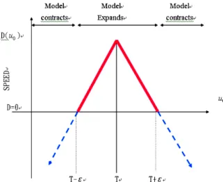
(2) manual operation, it is demonstrated that the proposed method is effective and efficient than manual selection of parameters. The experimental results demonstrate the effectiveness of our viewpoint. This proposed algorithm increases the efficiency for Threshold Level Set because of automatic optimal parameter selection.. surface to have less area (and remain smooth), and α ∈ 0,1 is a free parameter that controls the degree of smoothness in the solution. The speed function at any one point is based solely on the input intensity u 0 at that point:. [ ]. D(u 0 ) = ε − | u 0 − T | 2. Threshold Level Set Method. Where u0 is the image intensity and the speed. The Level Set formulation is based on the observation due to Osher and Sethian. A curve Γ(t ) can be seen as the zero-level of a function in higher. dimension. φ ( x, t ). .. The. evolving. function φ ( x, t ) which contains the embedded motion of. Γ(t ) as the level-set {φ = 0} and the evolving. function φ is always zero on the propagating hyper surface. Fig .1 shows the outward propagation of an initial curve and the accompany motion of the level set function φ .. 2.1. ∂φ v v = − ∇φ n ⋅ v ∂t v dx r dy r v ∇φ and v = i + j. With n = dt dt ∇φ. (1). Threshold Level Set Method. The Threshold level set model [23], let F = n ⋅ v , F can be design as follow:. F = −(αD(u0 ) + (1 − α )∇ ⋅. function is D (u 0 ) as shown in Fig. 2.; T − ε denots. LowerThreshold, T + ε denots UpperThreshold. The values of speed function are always zero when the intensity of image equals to T − ε or T + ε . The stop location of active contours is controlled by adjusting values of LowerThreshold and UpperThreshold. The UpperThreshold parameter can make the curve capture the boundary of cerebrospinal fluid and white matter. The LowerThreshold parameter can make the curve capture the boundary of the gray matter and white matter.. 3. Level Set Method. In this section, we describe the main idea of the Level Set Methods. The evolving function φ ( x, t ) is subjected to the evolution equation as follows:. 2.2. (4). ∇φ ) | ∇φ |. (2). and the level set equation can be expressed as follow:. ∂φ ∇φ = ∇φ (αD(u 0 ) + (1 − α )∇ ⋅ ) ∂t | ∇φ |. (3). Parameter. Selection. For MRI image segmentations, Otsu method is used in the adaptive parameter selection algorithm to obtain the parameters of level set to capture the contours of white matter. The adaptive threshold algorithm is described as follows: 1. Set n=3; 2. While (n>0) N=the threshold is calculated by Otsu method; Switch n Case 1: LowerThreshold=N; n=n-1; Case 2: If (intensity of image > N) then set intensity to zeros; Creation of modified histogram; n=n-1; UpperThreshold=N; Case 3: If (intensity of image < N) then set intensity to zeros; Creation of modified histogram; n=n-1; End switch; End while;. where D is a data term that forces the model toward desirable features in the input data, the term ∇ ⋅. The Adaptive Algorithm. ∇φ | ∇φ |. is the mean curvature of the surface, which forces the. - 1330 -.

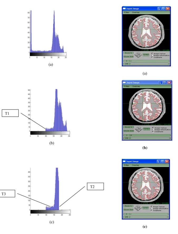
(3) 4. Experiment Results. References. National Library of Medicine Insight Segmentation and Registration Toolkit (ITK)[24] is an open-source software system to support the Visible Human Project. The Threshold Segmentation LevelSet program Module in ITK is used for the experiments. Otsu method is embedded in the adaptive algorithm to calculate optimal values of threshold parameters. The brain MRI image is shown in Fig. 3(a) and the image is smoothed shown in (b) and its histogram as shown in Fig. 4(a). We use the example to explain the adaptive parameter selection Algorithm. By using Otsu method and the smoothed image Fig. 3(b), we get the threshold T1. The modified histogram Fig. 4(b) is obtained by setting the gray level equal to zero those value are less than T1. By using Otsu method and the modified histogram Fig. 4(b), we get the threshold T2. The modified histogram Fig. 4(c) is obtained by setting the gray level equal to zero those value are larger than T2. By using Otsu method and the modified histogram Fig. 4(c), we get the threshold T3. The values of LowerThreshold and UpperThreshold are set T3 and T2. It is very consuming time to obtain manually the values of parameters. The optimal parameters, LowerThreshold=145 and UpperThreshold=182, was obtained by our algorithm. It is also important to evaluate the influence ofα. Fig. 5 shows segmentation result with (a)α=0.2, (b)α=0.5 and (c) α=0.8 and the value of optimal parameters. As α is increased, the weight value (1- α ) of the Curvature term is decreased. The cave boundary of the contour of brain white matter is large and it is easy to be captured by less value of α.. 5. Conclusions and Feature Work. The adaptive parameter selection algorithm using Otsu method for automatic selection of the LowerThreshold and UpperThreshold of Threshold Level Set is presented. The UpperThreshold parameter can make the curve capture the boundary of cerebrospinal fluid and white matter. The LowerThreshold parameter can make the curve capture the boundary of the gray matter and white matter.. Acknowledgments I would like to thank the Department of medical imaging and radiological sciences supporting for the study. With gratitude US National Library of Medicine of the National Institutes of Health States provides the ITK to use for everybody.. 1. Kass, M., Witkin, A. and Terzopoulos, D,: Snakes: Active contour models, International Journal of Computer Vision (1988) 321–331. 2. Terzopoulos, D. (1986a). “On matching Deformable Models to Images.”Tech.rept. 60. Schlumberger Palo Alto Research. Reprinted in Topical Meeting on Machine Vision, Technical Digest Series, Vol.12,(Optical Society of America, Washington,DC) 1987, 160-167. 3. Terzopoulos, D,. Witkin, A. and Kass, M. (1988).: Constraints on deformable models: Recovering 3D shape and nonrigid motion.”Artif. Intelligence, Vol.36, No.1, pp.91-123. 4. Terzopoulos, D. and Fleischer, K.(1988).: Deformable models. The Visual Computer, Vol.4, No.6,pp.306-331. 5. F. Leymarie and M. D. Levine. “Tracking deformable objects in the plane using an active contour model.” IEEE Trans. on Pattern Anal. Machine Intell., 15(6):617-634, 1993. 6. McInerney, T. & Terzopoulos, D. (1996). “On matching Deformable Models to Images.” Medical Image Analysis, Vol.1, No.2, pp. 91-108. 7. R. Malladi, J. A. Sethian, and B. C. Vemuri. “Shape modeling with front propagation: A level set approach.”IEEE Trans. on Pattern Anal. Machine Intell., 17(2):158-175, 1995. 8. S. Osher and J. A. Sethian. “Fronts propagating with curvature-dependent speed: Algorithms based on Hamilton-Jacobi formulations.”Journal of Computational Physics, 79:12-49, 1988. 9. V. Caselles. “Geometric models for active contours.”In Proceedings of the 1995 IEEE International Conference on Image Processing, volume 3, pages 9-12, 1995. 10. C. Xu and J. L. Prince, “Snakes, shapes and gradient vector flow,” IEEE Trans. Image Processing, vol. 7, pp. 359–369, Mar. 1998. 11. Zeyun Yu and Chandrajit Bajaj,Image Segmentation Using Gradient Vector Diffusion and Region Merging,Department of Computer Science, University of Texas as Austin,Austin,Texas 78712,USA.[12]Osher, Fedkiw, "Level Set Methods and Dynamic Implicit Surfaces", Springer Verlag, 2002. 13. J.A. Sethian, Level Set Methods. Cambridge University Press, 1996. 14. Guillermo Sapiro, Geometric Partial Differential Equations and Image Analysis. Cambridge, University Press, 2001. 15. G. Evans, J. Blackledge, P. Yardley, Numerical Methods for Partial Differential Equations, Springer. 16. D. Mumford and J. Shah, “Optimal approximation by piecewise smooth functions and associated variational problems,” Commun. Pure Appl. Math, vol. 42, pp. 577–685, 1989. 17. R. Malladi, J. A. Sethian, and B. C. Vemuri, “Shape modeling with front propagation: A level set approach,” IEEE Trans. Pattern Anal. Machine Intell., vol. 17, pp. 158–175, Feb. 1995. 18. V. Caselles, F. Catté, T. Coll, and F. Dibos, “A geometric model for active contours in image processing,” Numer. Math., vol. 66, pp. 1–31, 1993. 19. V. Caselles, R. Kimmel, and G. Sapiro, “On geodesic active contours,” Int. J. Comput. Vis., vol. 22, no. 1, pp. 61–79, 1997. 20. S. C. Zhu, T. S. Lee, and A. L. Yuille, “Region competition: unifying snakes, region growing,. - 1331 -.

(4) energy/bayes/MDL for multi-band image segmentation,” in Proc. IEEE 5th Int. Conf. Computer Vision, Cambridge, MA, 1995, pp. 416–423. 21. S. Kichenassamy, A. Kumar, P. Olver, A. Tannenbaum, and A. Yezzy,“Gradient flows and geometric active contour models,” in Proc. Int. Conf. Computer Vision, Cambridge, MA, 1995, pp. 810–815. 22. K. Siddiqi, Y. B. Lauziére, A. Tannenbaum, and S.W. Zucker, “Area and length minimizing flows for shape segmentation,” IEEE Trans. Image Processing, vol. 7, pp. 433–443, Mar. 1998.. 23. Aaron E. Lefohn, Joshua E. Cates, Ross and T. Whitaker :Interactive, GPU-Based Level Sets for 3D Segmentation, Proceedings of Medical Image Computing and Computer Assisted Intervention (MICCAI) 2003. 24. Insight Toolkit (ITK),The National Library of Medicine Insight Segmentation and Registration Toolkit, http://www.itk.org/. (a) (a). (b). Fig. 1. The level set (a) evolution function and (b) the curve obtained with zero level of the level set function.. (b) Fig. 3. The (a) original image and (b) smoothed image.. Fig. 2. The speed function D (u 0 ) is a function of intensity u 0 .. - 1332 -.

(5) (a) (a). T1. (b) (b). T2 T3. (c) (c) Fig. 4. (a) is the histogram of the smoothed image and (b) (c) are the modified histograms.. Fig. 5. The contours are obtained with various α value (a) α=0.2 (b) α=0.5 and (c) α=0.8. - 1333 -.

(6)