Liquidity Cost of Market Orders in Taiwan Stock Market: A Study based on An Order-Driven Agent-Based Artificial Stock Market

1

Liquidity Cost of Market Orders in Taiwan Stock Market: A Study based

on An Order-Driven Agent-Based Artificial Stock Market

Yi-ping Huanga∗, Shu-Heng Chenb, Min-Chin Hunga

a

Department of Financial Engineering and Actuarial Mathematics, Soochow University

b_{Department of Economics, National Chengchi University}

Abstract

This thesis construct an order-driven artificial stock market base on Daniels et al. (2003) model. We also use autoregressive conditional duration (ACD) model initiated by Engle and Russell (1998) to model duration or order size. We analyzed the

transaction cost of ten securities, including stocks, Exchange-Traded Funds (ETFs) and Real Estate Investment Trusts (REITs), in Taiwan stock market and compared this result with the simulated cost of our models. We find that for those frequently traded securities, for example, TSMC (2330.TW) or China Steel (2002.TW), it is better not to incorporate ACD model of duration in the model, and for those not frequently traded securities, for example, President Chain Store (2912.TW) or Gallop No.1 Real Estate Investment Trust Fund (01008T.TW), it is better to incorporate ACD model of duration in the model. Our empirical estimates show that the liquidity costs of market order of these ten securities are generally smaller than 3%, and largely lied between -1% and 1%. We, however, find that simulation costs of market orders in our model, with a range from 0% to 10%, are generally larger than those of real data. One possible reason for this departure is that investors in stock markets generally do not place their orders blindly. They tend to wait for the appearance of opposite order size, and then place their orders. They also tend to split up a large order, and then reduce market impact. These behavior do not exist in our simulation. Regardless of these differences, our models may still be a simulation tool for transaction cost assessment when one would like to liquidate their asset in a short span of time.

Key Words：：：：Order-Driven, Liquidity, Transaction Cost.

∗

Corresponding author. Contact address: 10692, 45 Lane 265 Hsin Yi Rd. Sec.4, Taipei, Taiwan. E-mail: b86704010@yahoo.com.tw

1. Introduction

1.1 Motivations

The liquidity cost (also called ”transaction cost”) in this study means the cost paid by stock market participants when they buy or sell their securities in stock market. Definitely speaking, the “cost” is the difference between the trading value an investor observed and the trading value they actually done. Especially for institutional investors or those who have large amount of trading position, they usually have large impact on the deal prices, liquidity cost is the topics they cannot neglect.

One of the objectives of the stock market is providing liquidity to securities holders and securities buyers, i.e. investors can buy those securities they would like to buy and securities holders can liquidate their securities in stock market. Nonetheless, various kinds of securities listing in the stock market, the trading activity between them differ from one another. Not all securities have good liquidity, some securities have a large trade volume, and some securities even do not have a trade at all in a trading day. Business cycle, rumors or news in financial market and order flow, these factors also affect the liquidity of a security from time to time.

For a security holder, if there is no enough buy orders in stock market, he may not smoothly liquidate his holdings. If this situation happens, the difference between his holding value calculated by market price multiply by shares of holdings and the market value he actually get after liquidation may be large. For corporate investors, the purpose of investment is increasing return of idle cash before expenditure for business activity, if investment holdings cannot be liquidated well, they might liquidate their holdings with large discount in order to match the business activity cash demand, and arises the “liquidity risk” in risk management regime. For the buyers, if there are no sufficient sell orders in the stock market, they cannot estimate how much cost they should paid for the buying.

“Financial tsunami” which began in mid-2007 showed that the poor liquidity resulted in suddenly and severely liquidity risk of financial institutes. Therefore, the liquidity of financial institution became an important topic of financial supervision after global financial crisis. Basel Committee on Banking Supervision（2009）of Bank for International Settlements has issued two regulatory standards on liquidity risk of banks on December, 2009. One of which1 is “Liquidity Coverage Ratio”：

1

3 100% period time day -30 a over outflows cash Net assets liquid quality high of Stock ≥

This ratio aims to ensure that the assets of a bank can liquidate to meet its

liquidity needs for a 30-day time horizon under severe liquidity stress scenario. In this regulatory standard, “high quality liquid assets” have fundamental characteristics, for example low credit and market risk, easy to valuation, etc., and market characteristics, including active and sizable market, i.e. a large number of market participants and a high trading volume, and good market breadth (price impact per unit of liquidity), market depth (units of the asset can be traded for a given price impact).

In recent years, the techniques of generating“trading strategies”or“buy/ sell signals”from analyzing historical market time series by using various computer software or artificial intelligence gradually become popular among investors. But these techniques always neglect the trading amount and market liquidity, i.e. they always do not take in to account the possibilities of extra transaction cost paid by investors which comes from poor liquidity of financial market.

In order to lower the transaction cost when buying or selling securities in stock market, the assessment of liquidity of a security is important in real situations of security trading, risk management and testing of a trading strategy. For financial institutions, how to evaluate the liquidity of assets in order to meet the requirement of new financial supervision standards is also an important topic. But stock market is a complex system, historical information might be only a outcome of many possibilities. We might fall into the fallacy of “naïve empiricism” if we only analyze liquidity from historical data. Therefore, this study build three simple order-driven agent-based artificial stock market models, and hope in the future we can analyze the investor’s transaction cost under different scenario by using these agent-based models.

1.2 Research objectives

The objectives of this study are as follows: first, build order-driven agent-based stock market models which are tailored to the matching rule employed by Taiwan Stock Exchange (TWSE). Second, based on our models, whether or not an investor can estimate the transaction cost when he want to liquidate a given amount of stock.

From a market participant’s point of view, we only try to estimate transaction cost under a given matching rule (call auction) in this study. We do not compare between different matching rules, for example, call auction and continuous auction, we also do not conclude which matching rule is better. Additionally, there is a “block transaction” rule in TWSE which is tailored for those orders which order size are larger than 500,000 shares. In practice, only those who can find counterparty first or

transfer shareholdings for financial planning, under these occasions, i.e. they have certain counterparty, then investors will trade under “block transaction” rule. For a common sell side, he may choose “call auction” rather than choose “block

transaction”, because his intention to sell stock may become known to the public when he try to find counterparty for “block transaction”, and may further affect or decrease the market price before he trade. Only trade by using “call auction” can hide his intention to sell. Therefore, from practical purpose and future applications point of view, in this study, we only analyze the transaction cost of market orders matching under “call auction” rule, we do not analyze the transaction cost of orders matching under “block transaction” rule.

1.3 Research framework

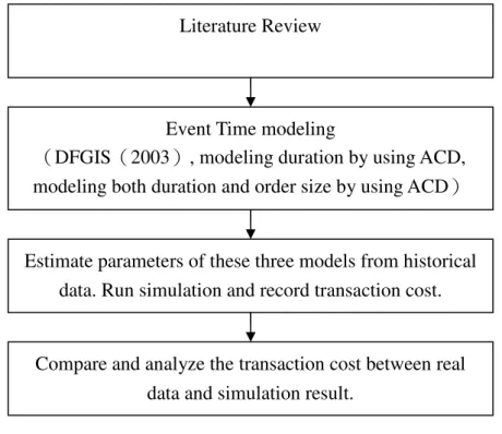
We review literature of order-driven agent-based model first. Based on the order-driven model proposed by Daniels, Farmer, Gillemot, Iori, Smith (2003), we build three order-driven event time stock markets comply with the matching rule employed by Taiwan Stock Exchange (TWSE). We estimate parameters of these models from historical data, and simulate trading. Finally, we compare historical transaction cost and simulated cost. Fig. 1 shows the framework of this study.

Fig. 1 Research framework

Literature Review

Event Time modeling

（DFGIS（2003）, modeling duration by using ACD, modeling both duration and order size by using ACD）

Estimate parameters of these three models from historical data. Run simulation and record transaction cost.

Compare and analyze the transaction cost between real data and simulation result.

5 2. Literature review

2.1. Agent-based models

Daniels et al. (2003) proposed an agent-based model which is not composed of many agents. They use five market parameters to build an order-driven stock market. These parameters including two order flow rates: limit order arrival rate (α), market order arrival rate (μ), and order cancelation rate (δ), average order size (σ), price tick size dp. Because of lacking rationality and learning, this is a zero intelligence agent-based model.

Farmer, Patelli and Zovko (2005a) tested Daniels et al. (2003) model with data from eleven stocks in London Stock Exchange in the period from August 1st 1998 to April 30 2000. They find that this order-driven model can do a good job of predicting or explaining spread and price impact curve.

Guo (2005) implemented a trading platform in Python based on Daniels et al.(2003) model (He called it “SFGK model”). This platform has an agent-based client-server framework, besides, it has a user interface for human to participate in trading. He tested the mid-price and spread of the model. He performed experiments of two liquidation strategies, and compared the transaction cost results.

2.2. Algorithmic trading

Algorithmic trading is an emerging topic in asset management industry. Broadly speaking, algorithmic trading contains using computer program to generate trading strategy or buy-sell signals, and automatic order submission. In academia, optimal execution strategy is a popular topic which is a topic about how to liquidate a given amount of securities at a minimum transaction cost.

In the literature of optimal execution, Almgren and Chriss (2000) mentioned “the total cost of trading” is the difference between the initial book value and the capture. They distinguished two kinds of market impact: temporary impact and permanent impact. Under the assumption that price impact functions are linear functions, they solved the constrained optimization problem, and derived the efficient frontier of optimal trading strategy which is the curve describe optimal trading strategy or minimum trading cost strategy for different risk-averse investors.

The difference between algorithmic trading literature and this study is that algorithmic trading literature always describes the optimal execution problem as an optimization problem. They cannot easily solve the problem without making some assumptions about price impact functions and stochastic process of stock price. In contrast to the algorithmic trading literature, this study use agent-based models for

trading cost simulation. The assumptions are more flexible in agent-based models than in solving optimization problems. We only need to make some assumptions about how to generate orders and cancel orders, and then we can simulate and analyze trading cost.

2.3. Autoregressive conditional duration model

Engle and Russell (1998) proposed the autoregressive conditional duration model (ACD model) for the analysis of irregular waiting times between transaction events (the time interval is called duration). This time series model can measure and predict density of events. They also found that this model can do a good job of

reducing Ljung-Box statistics of durations. They suggested joint modeling of volumes, transaction prices, and quotes would give better understanding of the fundamental mechanisms of time variation in liquidity of NYSE markets.

Manganelli (2002) suggested volume is a kind of clustering activities; therefore one can view volume as an autoregressive process. He suggested that it is plausible to model volume in a ACD fashion. Besides, volume and duration are both positive value variables. He called these models autoregressive conditional volume (ACV) models. The simplest ACV is an ACV(1,1):

t t t

φ

η

ν

η

(

σ

)

ω

αν

βφ

φ

Since volume

ν

η

variable. He tested this model on a sample of ten stocks traded in the NYSE. He found that for those frequently traded stocks, the autoregressive coefficients （β） are always above 0.9. He believed this finding indicate that the empirical regularities found for durations hold for volume as well.

3. Transaction cost analysis and the models

3.1. Transaction cost analysis

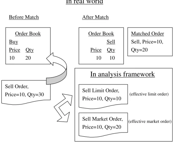
Before discussion about transaction cost analysis framework of this study, we review definition of effective market order and effective limit order first. In Daniels et al. (2003) model, only two types of order are allowed. One is market order the other is limit order which order price is not allowed to cross best bid price or best ask price, i.e. for a limit buy order, the price must be below the best ask price; for a limit sell order, the price must be above the best bid price. In stock market practice, the price of

7

limit orders may cross best price, and the number of order types are usually more than two. For simplicity of analysis and complying with Daniels et al. (2003) model, Farmer et al. (2005b) define effective market orders as shares that result in a trade immediately, and effective limit orders as shares that will leave shares in order book. They split orders that cross the opposing best price into effective market orders and effective limit orders by these definitions, and then calculate model parameters.

We define transaction cost as the difference between the amount of possible

transaction and amount of immediate transaction of an effective market order. We adopt the method applied by Farmer et al. (2005b) for splitting the orders that cross the opposing best price into effective market orders and effective limit orders, and calculate transaction cost of each effective market order that result in a transaction immediately.

Fig. 2 illustrates about how to split an order that cross the opposing best price. The best bid price is 10 and 20 shares. If a limit sell order arrives with price 10 and 30 shares, this order will result in a transaction with price 10 and 20 shares and leave 10 shares in the sell order book ceteris paribus. Thus, we split this 30 shares sell order into an effective market sell order with 20 shares and an effective limit sell order with 10 shares. Because of the split, mismatch between actual matching shares and

effective market shares may happen when we calculate the transaction amount from matching shares. If this situation happens, we use the shares of effective market order to calculate the transaction amount.

The amount of possible transaction is calculated by best price multiply by shares of effective order. This amount means the investor’s expectation transaction amount at next match. Hence, the transaction cost in this study can also be interpreted as the difference between investor’s expected transaction amount and actual transaction amount.

We neglect the orders arrive before the first disclosure in a trading date when we calculate the model parameters. Because the opposing best prices of these orders are not available, we cannot tell whether these orders are effective market orders or effective limit orders. Also, we neglect the orders after market close.

The amount of immediate transaction means that the effective market order must result in transaction at next match, and then we calculate transaction cost of this order. For those orders do not be matched at next match, the investors of these orders may pay some waiting cost. The transaction cost calculation is much more complex in this situation than in the situation of immediately transaction.

When limit up or limit down happens, i.e. best ask or best bid is not available, the new arrived buy order may be a limit buy order or a market buy order. In this situation, we classify this order into a market order or a limit order by a presumed probability. The presumed probability may be inaccurate. In our sample time intervals,

Order Book Buy Price Qty 10 20

Before Match After Match

Order Book Sell Price Qty 10 10 Matched Order Sell, Price=10, Qty=20 Sell Order,

Price=10, Qty=30 Sell Limit Order,

Price=10, Qty=10

Sell Market Order, Price=10, Qty=20

In real world

In analysis framework

(effective market order)

9

limit up or limit down only happen in a few trading days, therefore the calculation of number of effective market orders may only be affected slightly by the inaccuracy of presumed probability.

The percentage expression of transaction cost is defined as follows: X=expected number of shares of immediate transaction

For market buy orders, transaction cost is:

X ask best X ask best -X price trade × × ×

For market sell orders, transaction cost is:

X bid best X price trade X bid best × × − ×

Under call auction matching rule, transaction cost may be positive or negative by definition. The negative transaction cost means that investors get a better trade price than they expect and vice versa.

3.2. Transaction cost models: event time modeling

The zero intelligence agent-based models of this study base on the model

proposed by Daniels et al. (2003). Daniels et al. (2003) model is an event time model, i.e. the events in their model are not connected with real time. In the event time model, we substitute a series of events happen in a trading day for the trading hours of a trading day. Basically, there are three kinds of event: limit order placement (denoted byαin this study, denoted by “L” in event series), market order placement (denoted byμin this study, denoted by “M” in event series) and order cancelation (denoted by δin this study, denoted by “C” in event series). The calculation of model parameters also bases on events.

From the simulation point of view, the simulation base on event time and the simulation base on real time are equivalent in simulation results. For example, suppose that we simulate a series of events: LMLCL..., actually it is equivalent to the simulation base on real time: L...real time elapsed…M...real time elapsed…L...real time elapsed…C...real time elapsed…L…. The advantage of event time modeling is that we can save simulation time, i.e. we do not waste the time between events.

The model proposed by Daniels et al.（2003）is a continuous double auction zero intelligence agent-based model. The data employed here comes from TWSE. The matching rule employed by TWSE is “call auction”. The orders in TWSE match once every 25 seconds. The matching rule of the zero intelligence agent-based models of this study is also modified to have a call auction every 25 events if one event

represents one second. Hence, we add two kinds of events in our models: one is blank event (denoted by “N” in event series), the other is matching event (denoted by “T” in event series) for this modification. Suppose that one event represents one second, a

letter “E” represents an event, the event series in trading hours of TWSE can be represented by TEEEEEEEEEEEEEEEEEEEEEEEET...for example.

The types of order in this study are the same with the Daniels et al.（2003） model, only limit order and market order are allowed. The buy price of a limit buy order cannot higher than or equal to the best ask price, and the sell price of a limit sell order cannot lower than or equal to the best bid price. The difference between Daniels et al. (2003) model is that the prices of all orders are limited by the price change limit employed by TWSE which is the price change interval between closing price of previous trade day minus 7% and closing price of previous trade day plus 7%. Thus, in this study, the order price of buy market order is limit up, the order price of sell market order is limit down. The tick sizes of this study are also tailored to the tick sizes of TWSE.

Another difference among Daniels et al. (2003) model is that the best prices in simulation of this study are the unexecuted best bid price and unexecuted best ask price during last match, not actual best bid price and actual best ask price in order book. This difference result from that the stock market in TWSE is not a continuous auction market. TWSE match stock orders once every 25 seconds (i.e. call auction), and then disclose those best five unexecuted order prices and volumes. TWSE does not disclose any information about new arrival orders between 25 seconds, and stock market investors in TWSE have no way to obtain the real-time best prices in reality. We make this modification such that our models coincide with actual environment in TWSE.

The input parameters of our agent-based models are as follows: )

(α

p : ratio of limit order placements to number of events during the trading day. )

(µ

p : ratio of market order placements to number of events during the trading day.

) (δ

p : ratio of order cancelations to number of events during the trading day. The sum of probability of all kinds of events must be equal to 1. Hence, the ratio of blank event is determined after we have the three ratios above.

( )

µ

( )

δ

α

p n

p( )=1− ( )− − .

σ

σ

σ

2 2

− _{（Weisstein,}

2005）. The order size in our model is a positive integer, i.e. the order size should be multiple of 1,000 shares, and the maximum order size is 499,000 shares the same with the order size restriction in reality.

11

The methodology of model parameters estimation is based on Farmer et al. (2005b). We calculate model parameters day by day first, and then calculate mean values weighted by the daily number of events. This methodology implies an important assumption that the daily probability distributions of these parameters are identical. This is also an important assumption in this study.

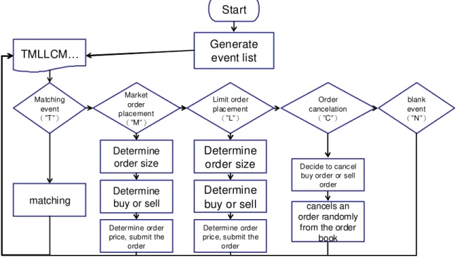
The computer program of this study is developed using Python Programming Language. The program generates series of events first, and then executes each event sequentially. If the event is a matching event (“T”) the program executes matching2. If the event is a market order placement (“M”) or a limit order placement (“L”) the program draws the order size, then decide buy order or sell order (the probability is 50% each), then submit the order. If the event is an order cancelation (“C”) the

program decides to cancel buy order or sell order3 (the probability is 50% each), then cancels an order randomly from the order book. If the event is a blank event (“N”) the program executes nothing and flows to next event. Fig. 3 is the flow chart of the program of our agent-based models.

Generate event list Matching event （”T”） TMLLCM… Market order placement （”M”） Order cancelation （”C”） blank event （”N”） Limit order plac ement （”L”） Determine order size Determine buy or sell Determine order price, submit the

order

Decide to canc el buy order or sell

order cancels an order randomly

from the order book matching Start Determine order size Determine buy or sell Determine order pric e, submit the

order

Fig. 3 Flow chart of our agent-based models

We have two methods to generate event list and we describe these methods as follows:

3.2.1 Determine event type by parameter directly

The first method is deciding types of each event sequentially according to the probability of each event (p(α)、p(μ)、p(δ)、p(n)). For example,

2

A general reference to the matching engine programming is Shetty and Jayaswal(2006).

3

TN=>TNL=>TNLM=>TNLML=>…. The probabilities of kinds of events are

calculated as follows: we calculate ratios of kinds of events day by day in our sample period, and then calculate mean values of these ratios weighted by the daily number of events. Since this method and the model are proposed by Daniels et al. (2003), we call this DFGIS model.

3.2.2 Determine duration by ACD model first, and then determine event type The second method is that we generate duration using autoregressive conditional duration model (ACD, Engle and Russell(1998)), and then decide event type

sequentially. For example, in the beginning we have an event list (if one event represents one second) filled with blank events between matching events, i.e. …TN NNNNNNNNNNNNNNNNNNNNNNNT…, and then we generate a duration list (x) using ACD model, and then discretize the durations, for example x=[…,1,2,3,4,…]. We can rewrite the original blank list to be …TE1E2NE3NNE4NNNE5...(a letter “E”

represents an event) by definition of duration, and then decide what kind of event sequentially by the probability of events (p(α)、p(μ)、p(δ)), for example if E1=L、

E2=M、E3=C、E4=L、E5=M. We can further rewrite the event list to be …TLMNCN

NLNNNM….

The parameters of ACD model are estimated as follows. We estimated ACD parameters from the durations of each trading day with EACD(1,1) model.

i i i x =ψ ε ( 3 ) 1 1 1 1 0 + − + − = _{i i} i α α x βψ ψ ( 4 )

ε is a random variable follows exponential distribution, its mean is 1. Since x_iis a positive value, we have to assume that α₀ >0,

α

β

The only difference between this model and DFGIS is that in the beginning of simulation, this model generate event list using ACD model. Since other parts of the model are the same with DFGIS model, we call this DFGIS-ACD model.

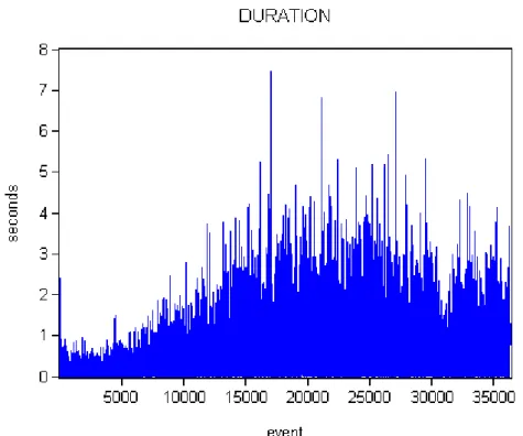
The reason of using ACD model as the DGP of duration is that this method may replicate the intraday pattern of duration. For example, Fig. 4 is the intraday durations of TSMC on April 17th 2008, the frequency of transaction is relatively high after market open and before market close, and the frequency of transaction is relatively low in the middle of a trading day. The DFGIS-ACD model may replicate this

13

inverted-U shape of durations, while the duration pattern in DFGIS model is purely random.

Fig. 4 Durations of TSMC(2330.TW) on April 17th 2008

3.2.3 Determine both duration and order size by ACD model

We find that for those thinly traded stocks the transaction cost in our simulation is generally higher than actual transaction cost. Since the matching rule, price ticks are the same with TWSE, we think that this difference may come from decision rules of order size, decision rules of buy or sell, order price and durations. For a thinly traded stock, if there is no enough opposing orders in order book, the transaction cost of a market order will be high. In reality, investors of thinly traded stock will wait until the opposing side has enough orders then they submit their market orders. Therefore, in order to approximate the effect of order size clustering, we think that it is plausible to model order size with autoregressive process the same with the idea proposed by Manganelli (2002). We build this model on the basis of DFGIS-ACD model, but in this model, we generate order size using EACD(1,1) model rather than draw a random variable from half-normal distribution. We call this model

4. Empirical data analysis and simulation result

4.1. Empirical data analysis result

In recent years, the securities listed in stock exchange are not only stock, warrant but also exchange traded fund (ETF) and real estate investment trust fund (REIT). ETF are baskets of stocks, and they are important vehicles of passive investment. Theoretically, REIT have better liquidity than holding real estate directly. Therefore, in addition to stocks we also include ETF and REIT as our samples of transaction cost analysis. The samples of this study are as follows: Taiwan Top50 Tracker Fund

(0050.TW), Polaris/P-shares Taiwan Dividend+ ETF (0056.TW), Cathay No.2 Real Estate Investment Trust (01007T.TW), Gallop No.1 Real Estate Investment Trust Fund (01008T.TW), China Steel (2002.TW), TSMC (2330.TW), MediaTek

(2454.TW), HTC (2498.TW), President Chain Store (2912.TW), Inotera (3474.TW). Table 1 shows the reasons of choosing these securities as our samples. The main purpose is that we hope the samples cover various characteristics as much as possible including high trading volume, low trading volume, high unit price and stocks for different risk appetites. All historical transaction data are provided by TWSE,

including daily order data, match data, disclose data. We use data from February 2008 to May 2008.

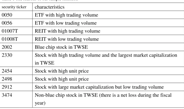
Table 1 The reasons of our sample selection security ticker characteristics

0050 ETF with high trading volume

0056 ETF with low trading volume

01007T REIT with high trading volume

01008T REIT with low trading volume

2002 Blue chip stock in TWSE

2330 Stock with high trading volume and the largest market capitalization in TWSE

2454 Stock with high unit price

2498 Stock with high unit price

2912 Stock with large market capitalization but low trading volume 3474 Non-blue chip stock in TWSE (there is a net loss during the fiscal

year)

If one event represents 0.01 seconds, the number of total events in a trading day is 1,620,000 (matching events are included). Table 2 shows the ratios of effective limit order, effective market order and order cancelation to total number of events (the number of matching events should be excluded) in a trading day and the average order

15

size of these 10 securities. The average order size of Taiwan Top50 Tracker Fund (0050.TW) is larger than TSMC (2330.TW) because the proportion of market participants is different. The market makers are the major participants of Taiwan Top50 Tracker Fund (0050.TW) while the participants of TSMC (2330.TW) are various kinds of investors. Although TSMC (2330.TW) is the largest market capitalization stock and traded frequently, the average order size is only 14,000 shares.

Table 2 the ratios of effective limit order, effective market order and order cancelation to total number of events(×10-3

) and the average order size

p(α) p(µ) p(δ) σ 0050 2.498 1.029 1.586 45 0056 0.404 0.147 0.232 19 01007T 0.109 0.059 0.042 21 01008T 0.026 0.010 0.003 22 2002 6.292 5.007 1.923 10 2330 6.676 5.059 2.218 14 2454 4.401 4.404 2.086 3 2498 2.570 2.404 1.182 3 2912 0.900 0.644 0.414 5 3474 1.195 0.960 0.459 ₁₁

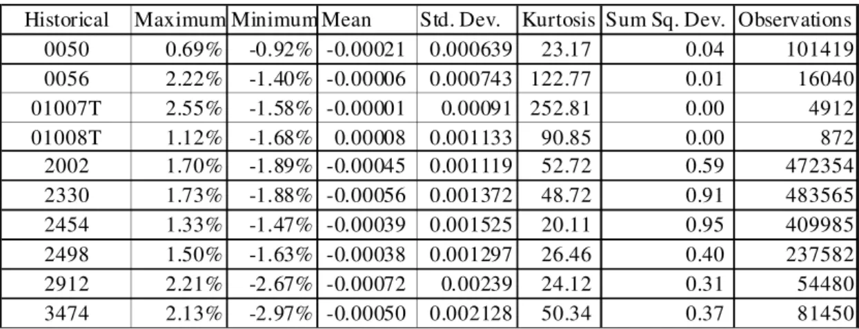
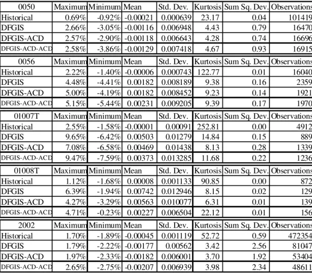
Table 3 shows the descriptive statistics of transaction cost of our samples.

Table 3 The descriptive statistics of transaction cost of our samples

Historical Maximum Minimum Mean Std. Dev. Kurtosis Sum Sq. Dev. Observations

0050 0.69% -0.92% -0.00021 0.000639 23.17 0.04 101419 0056 2.22% -1.40% -0.00006 0.000743 122.77 0.01 16040 01007T 2.55% -1.58% -0.00001 0.00091 252.81 0.00 4912 01008T 1.12% -1.68% 0.00008 0.001133 90.85 0.00 872 2002 1.70% -1.89% -0.00045 0.001119 52.72 0.59 472354 2330 1.73% -1.88% -0.00056 0.001372 48.72 0.91 483565 2454 1.33% -1.47% -0.00039 0.001525 20.11 0.95 409985 2498 1.50% -1.63% -0.00038 0.001297 26.46 0.40 237582 2912 2.21% -2.67% -0.00072 0.00239 24.12 0.31 54480 3474 2.13% -2.97% -0.00050 0.002128 50.34 0.37 81450

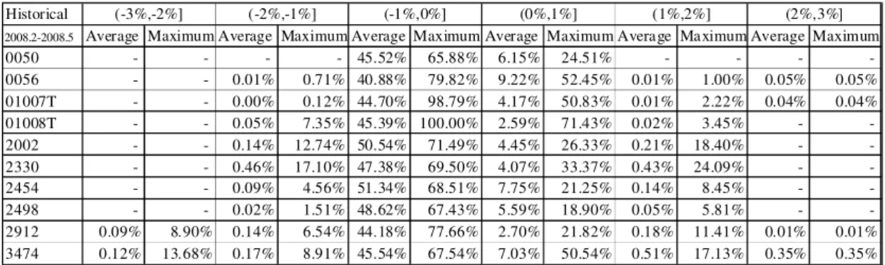
We group the transaction cost into classes and show the ratio of effective market orders which result in transaction immediately to total trade volume in Table 4.

Table 4 The ratios of effective market orders which result in transaction immediately to total trade volume in different classes

Historical

2008.2-2008.5 Average Maximum Average Maximum Average Maximum Average Maximum Average Maximum Average Maximum 0050 - - - - 45.52% 65.88% 6.15% 24.51% - - - -0056 - - 0.01% 0.71% 40.88% 79.82% 9.22% 52.45% 0.01% 1.00% 0.05% 0.05% 01007T - - 0.00% 0.12% 44.70% 98.79% 4.17% 50.83% 0.01% 2.22% 0.04% 0.04% 01008T - - 0.05% 7.35% 45.39% 100.00% 2.59% 71.43% 0.02% 3.45% - -2002 - - 0.14% 12.74% 50.54% 71.49% 4.45% 26.33% 0.21% 18.40% - -2330 - - 0.46% 17.10% 47.38% 69.50% 4.07% 33.37% 0.43% 24.09% - -2454 - - 0.09% 4.56% 51.34% 68.51% 7.75% 21.25% 0.14% 8.45% - -2498 - - 0.02% 1.51% 48.62% 67.43% 5.59% 18.90% 0.05% 5.81% - -2912 0.09% 8.90% 0.14% 6.54% 44.18% 77.66% 2.70% 21.82% 0.18% 11.41% 0.01% 0.01% 3474 0.12% 13.68% 0.17% 8.91% 45.54% 67.54% 7.03% 50.54% 0.51% 17.13% 0.35% 0.35% (1%,2%] (2%,3%] (-3%,-2%] (-2%,-1%] (-1%,0%] (0%,1%]

The results presented in Table 2, Table 3 and Table 4 show that no matter how dense the events are (or transactions), the transaction costs largely lies between -1% and +1%, and the immediately traded effective market orders in these classes are averagely more than 50% of daily trade volume. The maximum transaction cost for an effective market order is smaller than 3%.

4.2. Agent-based models simulation and result 4.2.1. Model parameters

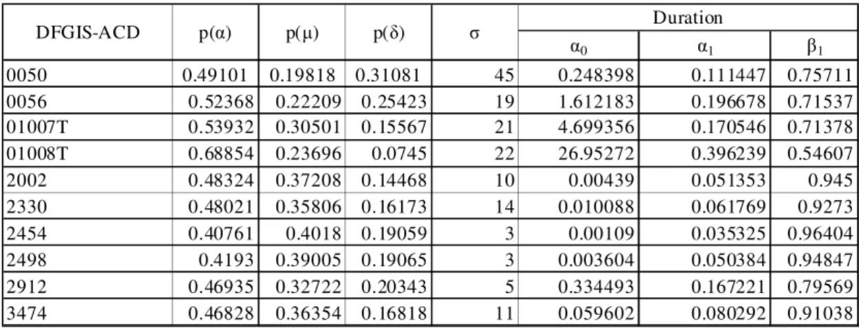
Table 5, Table 6, and Table 7 show the parameters of DFGIS model,

DFGIS-ACD model and DFGIS-ACD-ACD model respectively. The average order size

σ

Table 5 Model parameters of DFGIS model

DFGIS p(α) p(µ) p(δ) σ 0050 0.002498 0.001029 0.001586 45 0056 0.000404 0.000147 0.000232 19 01007T 0.000109 0.000059 0.000042 21 01008T 0.000026 0.00001 0.000003 22 2002 0.006292 0.005007 0.001923 10 2330 0.006676 0.005059 0.002218 14 2454 0.004401 0.004404 0.002086 3 2498 0.00257 0.002404 0.001182 3 2912 0.0009 0.000644 0.000414 5 3474 0.001195 0.00096 0.000459 11

17 Table 6 Model parameters of DFGIS-ACD model

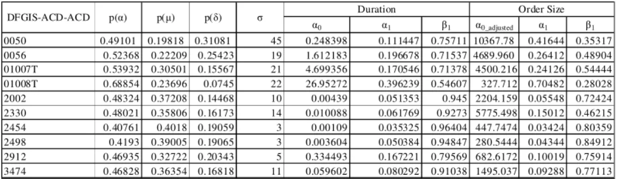
α0 α1 β1 0050 0.49101 0.19818 0.31081 45 0.248398 0.111447 0.75711 0056 0.52368 0.22209 0.25423 19 1.612183 0.196678 0.71537 01007T 0.53932 0.30501 0.15567 21 4.699356 0.170546 0.71378 01008T 0.68854 0.23696 0.0745 22 26.95272 0.396239 0.54607 2002 0.48324 0.37208 0.14468 10 0.00439 0.051353 0.945 2330 0.48021 0.35806 0.16173 14 0.010088 0.061769 0.9273 2454 0.40761 0.4018 0.19059 3 0.00109 0.035325 0.96404 2498 0.4193 0.39005 0.19065 3 0.003604 0.050384 0.94847 2912 0.46935 0.32722 0.20343 5 0.334493 0.167221 0.79569 3474 0.46828 0.36354 0.16818 11 0.059602 0.080292 0.91038 Duration σ DFGIS-ACD p(α) p(µ) p(δ)

Table 7 Model parameters of DFGIS-ACD-ACD model

α0 α1 β1 α0 α1 β1 0050 0.49101 0.19818 0.31081 45 0.248398 0.111447 0.75711 15718.67 0.41644 0.35317 0056 0.52368 0.22209 0.25423 19 1.612183 0.196678 0.71537 6821.198 0.26412 0.48904 01007T 0.53932 0.30501 0.15567 21 4.699356 0.170546 0.71378 5768.225 0.24126 0.54444 01008T 0.68854 0.23696 0.0745 22 26.95272 0.396239 0.54607 4824.83 0.70482 0.28028 2002 0.48324 0.37208 0.14468 10 0.00439 0.051353 0.945 2204.159 0.05548 0.72424 2330 0.48021 0.35806 0.16173 14 0.010088 0.061769 0.9273 5775.498 0.15012 0.46215 2454 0.40761 0.4018 0.19059 3 0.00109 0.035325 0.96404 447.7474 0.03424 0.80359 2498 0.4193 0.39005 0.19065 3 0.003604 0.050384 0.94847 280.5444 0.04344 0.84912 2912 0.46935 0.32722 0.20343 5 0.334493 0.167221 0.79569 682.6172 0.10019 0.75914 3474 0.46828 0.36354 0.16818 11 0.059602 0.080292 0.91038 1495.037 0.09288 0.77113

DFGIS-ACD-ACD p(α) p(µ) p(δ) σ Duration Order Size

The duration parameters of DFGIS-ACD model and the order size parameters of DFGIS-ACD-ACD model are estimated using EACD(1,1) model, and are weighted average of appropriate daily estimates. Furthermore, under the assumption of weakly stationary, the average order size is the function of order size parameters, i.e. the average order size μorder_size can be expressed as:

1 1 0 _ 1 α β α µ − − = size order _{( 5 )}

We can calculateμorder_size from Eq. ( 5 ) using order size parameters provided by

Table 7 and compare with

σ

order_size is obviously larger than

σ

eliminate the effect of this deviation, we adjust α₀ of order size parameters such that

0

α and

σ

Table 8 Model parameters of DFGIS-ACD-ACD model (after we adjust α₀ in Order Size) α0 α1 β1 α0_adjusted α1 β1 0050 0.49101 0.19818 0.31081 45 0.248398 0.111447 0.75711 10367.78 0.41644 0.35317 0056 0.52368 0.22209 0.25423 19 1.612183 0.196678 0.71537 4689.960 0.26412 0.48904 01007T 0.53932 0.30501 0.15567 21 4.699356 0.170546 0.71378 4500.216 0.24126 0.54444 01008T 0.68854 0.23696 0.0745 22 26.95272 0.396239 0.54607 327.712 0.70482 0.28028 2002 0.48324 0.37208 0.14468 10 0.00439 0.051353 0.945 2204.159 0.05548 0.72424 2330 0.48021 0.35806 0.16173 14 0.010088 0.061769 0.9273 5775.498 0.15012 0.46215 2454 0.40761 0.4018 0.19059 3 0.00109 0.035325 0.96404 447.7474 0.03424 0.80359 2498 0.4193 0.39005 0.19065 3 0.003604 0.050384 0.94847 280.5444 0.04344 0.84912 2912 0.46935 0.32722 0.20343 5 0.334493 0.167221 0.79569 682.6172 0.10019 0.75914 3474 0.46828 0.36354 0.16818 11 0.059602 0.080292 0.91038 1495.037 0.09288 0.77113

DFGIS-ACD-ACD p(α) p(µ) p(δ) σ Duration Order Size

4.2.2. Trade volume(shares) and number of transactions

We compare the weighted average of trade volume (shares) and number of transactions between sample data and simulation data of the three models, as shown in Table 9. We find that the results of the DFGIS model are generally larger than the sample data while the results of the DFGIS-ACD model and DFGIS-ACD-ACD model are generally smaller than DFGIS model. The reason of the larger trade volume of the models may be that the order sizes of market orders in the models are larger than actual market order sizes. When investors employ algorithmic trading, i.e. a large size market order will be split into many small size market orders, average order size of market order may be obviously smaller than limit order, but we does not calculate the average order size of market orders and limit orders respectively. Therefore, in simulation, we may overvalue the order size of market orders when we draw random variables (i.e. order size) from half-normal distribution with mean

σ

19 Table 9 Comparison between trade volume (shares) and number of transactions between sample data and simulation data

Trade Volume(Share) Transaction Trade Volume(Share) Transaction

Historical 15,411,781 2,554 1,438,702 352

DFGIS 73,289,200 2,997 5,334,100 506

DFGIS-ACD 73,234,700 2,898 4,576,400 418

D FGIS-ACD-ACD 74,186,000 3,038 4,875,500 437

Trade Volume(Share) Transaction Trade Volume(Share) Transaction Historical 1,731,457 144 332,438 24

DFGIS 2,136,900 190 447,200 34

DFGIS-ACD 2,927,500 271 420,100 35

D FGIS-ACD-ACD 2,686,700 259 175,900 32

Trade Volume(Share) Transaction Trade Volume(Share) Transaction

Historical 69,341,433 12,582 3,228,883 1,369

DFGIS 95,335,300 12,765 5,120,400 1,819

DFGIS-ACD 74,326,200 11,315 3,267,900 1,169

D FGIS-ACD-ACD 79,122,100 11,874 3,289,100 1,278

Trade Volume(Share) Transaction Trade Volume(Share) Transaction

Historical 6,475,480 4,332 12,749,066 8,010

DFGIS 10,357,200 4,788 17,604,900 7,809

DFGIS-ACD 8,300,800 4,227 12,638,000 6,381

D FGIS-ACD-ACD 6,039,900 3,460 14,559,000 7,685

Trade Volume(Share) Transaction Trade Volume(Share) Transaction

Historical 50,360,139 12,062 11,124,524 2,183 DFGIS 64,442,500 11,826 15,510,000 2,794 DFGIS-ACD 46,743,400 9,762 11,258,500 2,087 D FGIS-ACD-ACD _{44,904,700 9,834 9,809,100 1,847} 0050 0056 01007T 01008T 3474 2002 2912 2330 2498 2454

4.2.3. Liquidity transaction cost analysis

We tabulate the descriptive statistics of transaction cost of historical data and the three models as shown in Table 10. Obviously, the transaction costs generated by the models are larger than sample data. This result may also result from the market order size difference between historical data and the models. The larger order sizes in the models result in the larger trade volumes and transaction costs than historical data.

If we evaluate the models by the dispersion of simulation results relative to historical data, i.e. we calculate the range between historical extrema and simulatin

extrema as Eq. ( 6 ):

actual simulated

actual

simulated -max min min

max + − _{( 6 )}

The smaller value in Eq. ( 6 ) the better the model is. The DFGIS model performs well in Polaris/P-shares Taiwan Dividend+ ETF (0056.TW), China Steel (2002.TW), TSMC (2330.TW), MediaTek(2454.TW) and HTC(2498.TW). The DFGIS-ACD model performs well in Taiwan Top50 Tracker Fund (0050.TW), Cathay No.2 Real Estate Investment Trust (01007T.TW), Gallop No.1 Real Estate Investment Trust Fund (01008T.TW), President Chain Store (2912.TW) and Inotera(3474.TW). The DFGIS-ACD-ACD model does not perform well in any securities, although it seems to increase kurtosis in some thinly traded securities, including Cathay No.2 Real Estate Investment Trust (01007T.TW), Gallop No.1 Real Estate Investment Trust Fund (01008T.TW), President Chain Store (2912.TW).

Table 10 The descriptive statistics of transaction cost of historical data and the three models

0050 MaximumMinimum Mean Std. Dev. Kurtosis Sum Sq. Dev. Observations

Historical 0.69% -0.92% -0.00021 0.000639 23.17 0.04 101419

DFGIS 2.66% -3.05% -0.00116 0.006948 4.43 0.79 16470

DFGIS-ACD 2.57% -2.90% -0.00118 0.006643 4.28 0.74 16696

DFGIS-ACD-ACD _{2.58% -3.86% -0.00129 0.007418 4.67 0.93 16915}

0056 Maximum Minimum Mean Std. Dev. Kurtosis Sum Sq. Dev. Observations

Historical 2.22% -1.40% -0.00006 0.000743 122.77 0.01 16040

DFGIS 4.48% -4.41% 0.00182 0.008189 9.38 0.16 2359

DFGIS-ACD 5.00% -4.19% 0.00182 0.008452 9.23 0.14 1921

DFGIS-ACD-ACD _{5.15% -5.44% 0.00231 0.009205 9.39 0.17 1970}

01007T Maximum Minimum Mean Std. Dev. Kurtosis Sum Sq. Dev. Observations

Historical 2.55% -1.58% -0.00001 0.00091 252.81 0.00 4912

DFGIS 9.65% -6.42% 0.00503 0.01279 14.84 0.15 889

DFGIS-ACD 7.08% -6.58% 0.00469 0.01438 8.13 0.28 1339

DFGIS-ACD-ACD _{9.47% -7.59% 0.00373 0.013285 11.68 0.22 1236}

01008T Maximum Minimum Mean Std. Dev. Kurtosis Sum Sq. Dev. Observations

Historical 1.12% -1.68% 0.00008 0.001133 90.85 0.00 872

DFGIS 6.39% -1.94% 0.00742 0.012946 8.15 0.02 129

DFGIS-ACD 4.27% -3.29% 0.00563 0.010077 6.31 0.01 139

DFGIS-ACD-ACD _{4.71% -0.23% 0.00227 0.006504 22.12 0.01 156}

2002 Maximum Minimum Mean Std. Dev. Kurtosis Sum Sq. Dev. Observations

Historical 1.70% -1.89% -0.00045 0.001119 52.72 0.59 472354

DFGIS 1.79% -2.22% -0.00177 0.00562 3.42 2.56 81047

DFGIS-ACD 1.97% -2.33% -0.00182 0.006001 3.70 1.92 53404

21

2330 Maximum Minimum Mean Std. Dev. Kurtosis Sum Sq. Dev. Observations

Historical 1.73% -1.88% -0.00056 0.001372 48.72 0.91 483565

DFGIS 2.03% -2.35% -0.00209 0.006375 3.37 3.31 81490

DFGIS-ACD 2.35% -2.67% -0.00210 0.006751 3.49 2.91 63906

DFGIS-ACD-ACD 2.68% -3.16% -0.00240 0.007609 3.65 3.67 63479

2454 Maximum Minimum Mean Std. Dev. Kurtosis Sum Sq. Dev. Observations

Historical 1.33% -1.47% -0.00039 0.001525 20.11 0.95 409985

DFGIS 2.93% -3.62% -0.00275 0.008793 3.45 5.51 71213

DFGIS-ACD 4.04% -4.74% -0.00276 0.009238 4.54 4.07 47687

DFGIS-ACD-ACD 4.01% -4.86% -0.00286 0.009744 4.37 5.67 59724

2498 Maximum Minimum Mean Std. Dev. Kurtosis Sum Sq. Dev. Observations

Historical 1.50% -1.63% -0.00038 0.001297 26.46 0.40 237582

DFGIS 3.76% -4.65% -0.00305 0.011251 3.78 4.90 38727

DFGIS-ACD 4.82% -5.49% -0.00272 0.010957 4.59 3.62 30114

DFGIS-ACD-ACD 4.76% -5.46% -0.00296 0.011787 4.79 3.10 22346

2912 Maximum Minimum Mean Std. Dev. Kurtosis Sum Sq. Dev. Observations

Historical 2.21% -2.67% -0.00072 0.00239 24.12 0.31 54480

DFGIS 7.32% -11.11% -0.00111 0.015314 8.40 2.42 10320

DFGIS-ACD 6.00% -7.38% -0.00038 0.012509 9.89 0.98 6242

DFGIS-ACD-ACD 9.26% -9.71% -0.00070 0.014384 10.48 1.30 6264

3474 Maximum Minimum Mean Std. Dev. Kurtosis Sum Sq. Dev. Observations

Historical 2.13% -2.97% -0.00050 0.002128 50.34 0.37 81450

DFGIS 5.35% -6.43% -0.00284 0.015003 4.38 3.50 15556

DFGIS-ACD 5.15% -6.59% -0.00181 0.014359 5.23 2.13 10317

DFGIS-ACD-ACD 6.03% -6.88% -0.00158 0.013863 5.74 1.71 8902

We group the simulated transaction cost into classes and show the ratio of effective market orders which result in transaction immediately to total trade volume in Table 11. Since the transaction costs disperse in a wide range (the maximum is 9.65%, the minimum is -11.11%), what we concern in this study is the cost paid by the investors, i.e. positive transaction costs , we group the negative and zero

transaction cost into one class, and tabulate the positive classes in detail in Table 11. We compare the simulated ratios with historical ratios, and find that DFGIS model performs well in Polaris/P-shares Taiwan Dividend+ ETF (0056.TW), Cathay No.2 Real Estate Investment Trust (01007T.TW), China Steel (2002.TW), TSMC

(2330.TW), MediaTek (2454.TW), and HTC(2498.TW). The DFGIS-ACD model performs well in Taiwan Top50 Tracker Fund (0050.TW), Gallop No.1 Real Estate Investment Trust Fund (01008T.TW), President Chain Store (2912.TW), and Inotera (3474.TW).

Table 11 The ratio of effective market orders which result in transaction immediately to total trade volume in different classes

0050

Average MaximumAverage MaximumAverage MaximumAverage MaximumAverage MaximumAverage Maximum Historical 45.52% 65.88% 6.15% 24.51% - - - -DFGIS 26.99% 30.88% 21.39% 23.52% 2.69% 3.68% 0.08% 0.41% - - - -DFGIS-ACD 27.19% 31.44% 22.34% 25.55% 2.41% 4.20% 0.10% 0.77% - - - -DFGIS-ACD-ACD24.45% 28.43% 21.37% 25.89% 4.33% 7.46% 0.46% 1.39% - - - -(0%,1%] (1%,2%] (2%,3%] (3%,4%] (4%,10%] (-12%,0%] 0056

Average MaximumAverage MaximumAverage MaximumAverage MaximumAverage MaximumAverage Maximum Historical 40.89% 79.82% 9.22% 52.45% 0.01% 1.00% 0.05% 0.05% - - - -DFGIS 13.53% 16.71% 22.70% 31.81% 5.09% 8.33% 1.11% 3.18% 0.28% 1.44% 0.06% 0.84% DFGIS-ACD 13.93% 17.18% 20.56% 28.06% 5.17% 9.95% 1.30% 4.35% 0.47% 2.73% 0.08% 0.92% DFGIS-ACD-ACD12.55% 16.26% 16.92% 23.50% 6.91% 11.95% 2.73% 8.46% 1.00% 4.68% 0.28% 3.02% (-12%,0%] (0%,1%] (1%,2%] (2%,3%] (3%,4%] (4%,10%] 01007T

Average MaximumAverage MaximumAverage MaximumAverage MaximumAverage MaximumAverage Maximum Historical 44.70% 98.79% 4.17% 50.83% 0.01% 2.22% 0.04% 0.04% - - - -DFGIS 13.51% 20.46% 17.21% 27.30% 7.72% 16.28% 3.28% 13.94% 1.57% 5.79% 1.26% 10.25% DFGIS-ACD 16.23% 21.25% 15.01% 25.74% 7.66% 14.17% 3.69% 8.02% 3.14% 7.60% 1.67% 8.10% DFGIS-ACD-ACD14.30% 21.55% 17.08% 26.97% 7.48% 16.94% 4.36% 10.43% 1.79% 6.02% 1.67% 8.87% (-12%,0%] (0%,1%] (1%,2%] (2%,3%] (3%,4%] (4%,10%] 01008T

Average MaximumAverage MaximumAverage MaximumAverage MaximumAverage MaximumAverage Maximum Historical 45.44% 100.00% 2.59% 71.43% 0.02% 3.45% - - - -DFGIS 9.25% 19.60% 13.14% 39.53% 4.42% 12.53% 3.25% 15.93% 2.09% 14.05% 2.94% 17.52% DFGIS-ACD 10.04% 26.91% 13.98% 34.52% 5.88% 24.77% 4.69% 24.59% 0.67% 7.62% 0.83% 10.26% DFGIS-ACD-ACD 7.87% 31.55% 3.66% 24.18% 0.99% 8.22% 1.14% 11.72% 1.08% 21.61% 0.92% 18.34% (-12%,0%] (0%,1%] (1%,2%] (2%,3%] (3%,4%] (4%,10%] 2002

Average MaximumAverage MaximumAverage MaximumAverage MaximumAverage MaximumAverage Maximum Historical 50.68% 73.56% 4.45% 26.33% 0.21% 18.40% - - - -DFGIS 44.06% 47.62% 20.85% 24.13% 1.21% 2.10% - - - -DFGIS-ACD 39.64% 42.87% 17.86% 21.75% 1.76% 3.52% - - - -DFGIS-ACD-ACD36.31% 41.51% 17.69% 21.68% 2.47% 4.32% 0.12% 0.36% - - - -(1%,2%] (2%,3%] (3%,4%] (4%,10%] (-12%,0%] (0%,1%] 2330

Average MaximumAverage MaximumAverage MaximumAverage MaximumAverage MaximumAverage Maximum Historical 47.84% 69.58% 4.07% 33.37% 0.43% 24.09% - - - -DFGIS 44.68% 47.26% 19.61% 22.27% 1.96% 3.13% 0.01% 0.19% - - - -DFGIS-ACD 41.76% 46.93% 18.25% 21.83% 2.30% 3.56% 0.03% 0.22% - - - -DFGIS-ACD-ACD39.51% 43.72% 18.66% 22.06% 3.01% 4.90% 0.25% 0.76% - - - -(-12%,0%] (0%,1%] (1%,2%] (2%,3%] (3%,4%] (4%,10%] 2454

Average MaximumAverage MaximumAverage MaximumAverage MaximumAverage MaximumAverage Maximum Historical 51.43% 68.51% 7.75% 21.25% 0.14% 8.45% - - - -DFGIS 45.68% 48.20% 20.48% 23.30% 4.54% 6.17% 0.40% 0.85% - - - -DFGIS-ACD 41.90% 49.15% 18.91% 22.43% 3.89% 6.18% 0.63% 2.00% 0.11% 0.74% 0.00% 0.03% DFGIS-ACD-ACD42.39% 45.43% 19.18% 24.27% 4.67% 6.61% 0.86% 2.02% 0.18% 0.84% 0.01% 0.25% (-12%,0%] (0%,1%] (1%,2%] (2%,3%] (3%,4%] (4%,10%] 2498

Average MaximumAverage MaximumAverage MaximumAverage MaximumAverage MaximumAverage Maximum Historical 48.64% 67.43% 5.59% 18.90% 0.05% 5.81% - - - -DFGIS 40.08% 45.71% 19.10% 23.10% 4.99% 7.58% 1.33% 3.61% 0.21% 0.75% - -DFGIS-ACD 39.31% 45.87% 17.58% 21.39% 4.31% 6.55% 1.14% 1.97% 0.27% 1.40% 0.03% 0.30% DFGIS-ACD-ACD33.90% 40.08% 16.56% 21.03% 4.36% 6.81% 1.55% 3.77% 0.49% 1.28% 0.03% 0.33% (-12%,0%] (0%,1%] (1%,2%] (2%,3%] (3%,4%] (4%,10%] 2912

Average MaximumAverage MaximumAverage MaximumAverage MaximumAverage MaximumAverage Maximum Historical 44.41% 77.66% 2.70% 21.82% 0.18% 11.41% 0.01% 0.01% - - - -DFGIS 29.49% 33.05% 18.31% 25.09% 4.31% 7.16% 2.16% 5.22% 1.03% 3.25% 0.74% 2.76% DFGIS-ACD 26.54% 30.56% 19.14% 26.14% 3.77% 6.27% 1.48% 4.85% 0.64% 3.19% 0.58% 2.30% DFGIS-ACD-ACD25.93% 34.18% 17.86% 25.80% 4.11% 7.42% 1.68% 6.05% 1.06% 2.72% 0.97% 3.58% (1%,2%] (2%,3%] (3%,4%] (4%,10%] (-12%,0%] (0%,1%]

23

3474

Average MaximumAverage MaximumAverage MaximumAverage MaximumAverage MaximumAverage Maximum Historical 45.84% 67.54% 7.03% 50.54% 0.51% 17.13% 0.35% 0.35% - - - -DFGIS 31.29% 36.02% 17.09% 20.48% 5.41% 6.85% 2.51% 3.85% 0.96% 2.00% 0.28% 0.72% DFGIS-ACD 28.15% 32.32% 15.58% 19.76% 5.42% 9.52% 2.48% 4.15% 0.93% 2.13% 0.21% 0.80%

DFGIS-ACD-ACD25.39% 28.85% 15.56% 22.07% 5.54% 7.98% 2.81% 5.94% 0.88% 2.55% 0.40% 1.57% (-12%,0%] (0%,1%] (1%,2%] (2%,3%] (3%,4%] (4%,10%]

The results of Table 10 and Table 11 show that in general, the DFGIS model performs well in those frequently traded securities (China Steel (2002.TW), TSMC (2330.TW), MediaTek (2454.TW) and HTC (2498.TW)), and the DFGIS-ACD model performs well in the relatively thinly traded securities (Taiwan Top50 Tracker Fund (0050.TW), Gallop No.1 Real Estate Investment Trust Fund (01008T.TW), President Chain Store (2912.TW), Inotera(3474.TW)).

The dispersion of simulated transaction costs is averagely larger than historical data. The frequency of events and matching rule of our agent-based models are the same with actual stock market. The major differences are permutation of events and market order price. In reality, investors in stock market generally do not place their orders blindly with limit up or limit down price, especially when they have large order size. They tend to wait for the appearance of opposing order size, and then place their market orders. This behavior is a reason for the smaller transaction cost in actual stock market. Another possible reason is that the market order sizes in our agent-based models may be larger than those in actual market, i.e. our models do not take the mitigation of price impact from the employment of algorithmic trading into account.

Our simulation results show that the attempt to model the behavior of clustering order placement (the DFGIS-ACD-ACD model) fail to meet our expectation. As Farmer et al.(2005b) state that the zero-intelligence models are not trying to claim that intelligence doesn’t play an important role in financial agents, these models provide a benchmark to separate properties that are driven by market institution from those driven by intelligent behavior, we believe that the actual distribution of transaction cost may be driven mainly by intelligence of stock market participants. If we hope that the simulation result to be closer to actual result, adding some intelligence (or order placement strategy) in the model seem inevitable.

In spite of some inaccuracies, our simulation results show how much transaction cost an impatient investor would pay if he would like to liquidate his security in a short span of time. For example, an investor’s shareholdings is 40% of daily trade volume, if he would like to liquidate his holdings in a trading day, the maximum transaction cost may be 2% to 3% instead of zero cost from historical result as shown in Table 11.

5. Conclusion and discussion

5.1. Conclusion

This study builds three simple order-driven zero intelligence agent-based artificial stock market models. These models are tailored to the trading rules employed by TWSE.

The samples of this study cover different investment vehicles and various characteristics. They are as follows: Taiwan Top50 Tracker Fund (0050.TW), Polaris/P-shares Taiwan Dividend+ ETF (0056.TW), Cathay No.2 Real Estate Investment Trust (01007T.TW), Gallop No.1 Real Estate Investment Trust Fund (01008T.TW), China Steel (2002.TW), TSMC (2330.TW), MediaTek (2454.TW), HTC (2498.TW), President Chain Store (2912.TW), Inotera (3474.TW). We use data from February 2008 to May 2008.

We compare the simulation transaction cost with actual transaction cost. All actual transaction costs are smaller than 3%, but the simulated transaction costs are much higher. The results show that investors do not submit market orders blindly, they may split a market order with large order size into many market orders with small order size or they may wait for the appearance of the opposing orders. But if an investor is eager to liquidate his holdings, i.e. he does not want to split his orders or wait for a long time, our models would be useful tools for transaction cost estimation in this situation. We also find that the DFGIS model performs well in frequently traded securities and DFGIS-ACD model performs well in securities not traded frequently.

The simulation results shown in Table 10 and Table 11 can be reference for the investors of these 10 securities. For example, if an investor’s shareholding is 15% of daily trade volume, he can liquidate his shareholding in one trading day without any transaction cost on the average. If he holds more than 50% of the daily trade volume and want to liquidate in a trading day, the maximum transaction cost may be 7%.

Limitation of this study is as follows: the models in this study can only estimate the transaction cost in common market condition. Joulin, Lefevre, Grunberg, and Bouchaud（2008）analyzed 893 stocks in NASDAQ and NYSE and found the relation between price jumps and news in Dow Jones using data from 2004 to 2006. They found that the price jumps are much more than the news. They believed that the spontaneous price jumps come from vanishing liquidity. The explanation of vanishing liquidity is as follows: liquidity providers place their limit order cautiously, and tend to cancel orders when uncertainty signals appear. Our models cannot estimate the

25

transaction cost in extremely pessimistic market condition with vanishing liquidity.

5.2. Suggestions for further research

Firstly, the parameter estimation in the DFGIS-ACD model using EACD(1,1) is a tentative experiment, it does not mean that EACD(1,1) is the best model. Although there are many extensions of ACD model, very few studies compare different ACD models using the same data (Pacurar, 2008). Hence, in the future we can incorporate different extensions of ACD model into our models.

Secondly, we assume the order size in DFGIS model and DFGIS-ACD model follows half-normal distribution, and in DFGIS-ACD-ACD model follows

exponential distribution. We find that the frequency of large order size in half-normal distribution is obviously smaller than actual data. As Fig. 5 shows, in the

DFGIS-ACD model, the order sizes are less than 300,000 shares, but the maximum order size could be 499,000 shares in reality. The growth of algorithmic trading in recent years results in the high frequency of specific order size (for example, 10, 20 or 50). For example, Fig. 6 shows that some market participants of Taiwan Top50

Tracker Fund (0050.TW) split their orders into many small orders with order size 10. In the future, we can simulate the order size using historical distribution instead of a common probability distribution.

Fig. 5 Comparison of order size between simulation and historical data. (Taiwan Top50 Tracker Fund (0050.TW) on March 20th 2008, and we only show the part in which order size larger than 50,000 shares)

Fig. 6 Split large orders into many small orders with order size 10. (Taiwan Top50 Tracker Fund (0050.TW) on March 20th 2008, and we only show the part in which order size smaller than 100,000 shares)

Thirdly, the models of this study have high flexibility, and it is easy to extend the models in many aspects. A more subtle calibration of model parameters may give better results. For example, if we would like to simulate the effect of algorithmic

27

trading, we can calibrate the order size parameter of market order and limit order respectively so that the market order and limit order have their own model parameters respectively in simulations. The parameters of ACD model can be estimated subtly so that the difference between simulated durations and actual durations can be eliminated. We can also calibrate the model parameters of buy order and sell order respectively so that we can simulate transaction cost in different market conditions, for example, strong buying and strong selling.

Another point is that the result of this study is “a priori knowledge”. We can further get “a posteriori knowledge” by performing experiments on different trading strategies in our models, and analyzing the transaction costs of these trading

strategies.

Finally, in order to achieve further improvement on efficiency of trading, TWSE changes from call auction to continuous auction step by step. The matching rule of warrants has employed continuous auction since June 28 2010. Therefore, the models of this study should be changed to continuous auction in the future. Furthermore, comparison of transaction cost between call auction and continuous auction can be made in order to be the reference for stock exchange when designing matching rules.

References

[1] Introduce of trading rules in the stock exchange market, Taiwan Stock Exchange Corporation, http://www.twse.com.tw/ch/trading/introduce/introduce.php。 [2] Almgren, R., and Chriss, N., 2000, Optimal execution of portfolio transactions,

Journal of Risk, 3：5-39.

[3] Basel Committee on Banking Supervision, 2009, International framework for liquidity risk measurement, standards and monitoring, Consultative Document,

Issued for comment by 16 April 2010, Bank For International Settlements.

[4] Daniels, M. G., Farmer, J. D., Gillemot, L., Iori, G., and Smith, E., 2003. Quantitative model of price diffusion and market friction based on trading as a mechanics random process. Physical Review Letters, 90

（10）:108102-1-108102-4.

[5] Engle R. F. and Russell, J. R., 1998. Autoregressive conditional duration: A new model for irregularly spaced transaction data. Econometrica, 66(5):1127-1162. [6] Farmer, J. D., Patelli, P., and Zovko, I. I., 2005a. The predictive power of zero

[7] Farmer, J. D., Patelli, P., and Zovko, I. I., 2005b. Supplementary material for ‘the predictive power of zero intelligence in financial markets’. PNAS USA, 102(6).

[8] Guo, T. X., 2005. An agent-based simulation of double-auction markets, Master Thesis of Graduate Department of Computer Science, University of Toronto. [9] Hetland, M. L., 2008. Beginning Python: From Novice to Professional（2nd

ed.）（pp.153）. Berkeley, CA：Apress.

[10] Joulin, A., Lefevre, A., Grunberg, D., and Bouchaud, J-P., 2008. Stock price jumps: News and volume play a minor role, Working paper,

http://arxiv.org/abs/0803.1769

[11] Manganelli, S., 2005. Duration, volume and volatility impact of trades, Journal

of Financial Markets, 8: 377-399.

[12] Meitz, M., and T. Teräsvirta, 2006. Evaluating models of autoregressive

conditional duration, Journal of Business & Economic Statistics, 24: 104-124. [13] Pacurar, M., 2008. Autoregressive conditional duration (ACD) models in

finance: A survey of the theoretical and empirical literature, Journal of

Economic Surveys, 22(4):711-751.

[14] Shetty, Y. and Jayaswal, S., 2006. Practical .NET for Financial Markets. Berkeley, CA：Apress.

[15] Tsay, R. S., 2008. Duration Models, Handout of Business 41910: Time Series Analysis for Forecasting and Model Building at the University of Chicago Booth School of Business.

http://faculty.chicagobooth.edu/ruey.tsay/teaching/uts/lec15-08.pdf

[16] Weisstein, E. W., 2005. "Half-Normal Distribution." From MathWorld--A Wolfram Web Resource.