二元損失管制圖之設計 - 政大學術集成

全文

(1)國立政治大學統計學系碩士學位論文. 指導教授：楊素芬博士. 立. 政治大. ‧ 國. 學. 二元損失管制圖之設計. ‧. Design of the Bivariate Loss Control Chart. n. er. io. sit. y. Nat. al. Ch. engchi. i n U. v. 研究生：呂雨築撰中華民國一百年六月.

(2) Acknowledgment 回想兩年來的日子，歷經前所未有的充實生活，無論是在知識、生活上皆有所成長。今天能夠與大家分享這兩年的成果與喜悅，一切都要感謝幫助、鼓勵及支持我的人。論文能如期順利的完成，首先要感謝的是我的指導老師楊素芬教授。兩年來，老師辛苦的指導與訓練，不僅僅讓我精進統計品管的知識，同時，老師也鼓勵我們要學以致用，將品管方法落實於生活。這段學習過程，我更懂得對於任何事都該負責任且保有積極的態度去面對。. 政治大. 感謝口試委員鄭惟孝、曾勝滄及黃榮臣教授，對於本論文仔細的審查檢閱並. 立. 給予精闢的見解，使得本論文能盡善盡美。. ‧ 國. 一起分享快樂與痛苦，感謝你們豐富我的研究所生活。. 學. 感謝陪伴我的同學及朋友，特別是鄭鈞遠、歐家玲和謝至芬，這段日子我們. ‧. 最後，我要感謝我最親愛的家人，溫暖的家始終是我的避風港。有你們的支. sit. y. Nat. 持，我的人生才是完整的。謝謝你們。. io. al. n. 及國立政治大學商學院研究團對補助，謹此致謝。. Ch. engchi. er. 本研究承蒙行政院國家科學委員會，計畫 NSC98-2118-M-004-005-MY2 補助. i n U. v. 呂雨築謹致中華民國一百年六月.

(3) ABSTRACT A single Bivariate loss chart to monitor both the mean vector and the covariance matrix of a process with two correlated quality characteristics is proposed. Unlike existing multivariate charts, our proposed control chart is based on bivariate average loss function. With this feature, we could monitor the average loss of the product. It was shown that the proposed loss chart could detect small changes in process parameters quickly. We compared the performance of the proposed chart with some multivariate charts, like Max Bivariate chart, Max CUSUM chart, MEWMA chart,. 政治大. EWMA M-chart, S chart and EWMA V-chart. Our proposed chart performs rather. 立. well when monitoring both the mean vector and the covariance matrix simultaneously.. ‧ 國. 學. An example is given to illustrate the proposed chart.. ‧. n. er. io. sit. y. Nat. al. Ch. engchi. i n U. v.

(4) Table of Contents Chapter 1 INTRODUCTION............................................................................... 1 1.1 The Importance of the Process Control......................................................... 1 1.2 Research Problem ........................................................................................ 1 1.3 Research Purpose ......................................................................................... 2 1.4 Literature Review ........................................................................................ 2 1.5 Proposed Method and Structure ................................................................... 8 Chapter 2 THE BIVARIATE LOSS CONTROL CHART.................................. 9 2.1 Design of the Bivariate Loss Chart ............................................................... 9 2.2 Average Bivariate Loss and its Distribution .................................................. 9 2.3 The Approximated Distribution of BL ......................................................... 11 2.4 The Control Limits of the BL Chart............................................................ 13 2.5 The Out-of-control Approximate Distribution of BL .................................. 14 2.6 Performance Measurement of the BL Chart................................................ 15 2.7 Illustrating Example of the Bivariate Loss Chart ........................................ 16 2.8 ARL1 of the Bivariate Loss Chart ............................................................... 26 2.9 The Bivariate Loss Chart with Optimal Sample Size and Sampling Interval 42 2.10 ATS1 Comparison of the Specified Bivariate Loss Chart and the Optimal Bivariate Loss Chart ................................................................................ 51. 立. 政治大. ‧. ‧ 國. 學. n. al. er. io. sit. y. Nat. Chapter 3 THE VSSI BIVARAITE LOSS CONTROL CHART .................... 56 3.1 Design of the VSSI Bivariate Loss Chart ................................................... 56 3.2 The Approximate Distribution of BL .......................................................... 57 3.3 The Control Limits of the VSSI BL Chart .................................................. 58 3.4 The Out-of-control Approximate Distribution of BL .................................. 59 3.5 Performance Measurement of the VSSI BL Chart ...................................... 59 3.6 Example for the VSSI Bivariate Loss Chart ............................................... 61 Chapter 4. Ch. engchi. i n U. v. ATS1 ANALYSIS OF THE VSSI BIVARIATE LOSS CHART AND ATS1 COMPARISON BETWEEN THE BL CHART AND THE VSSI BL CHART ............................................................................. 65. 4.1 The Specified ( nq , hq , p (nq ) ) VSSI Bivariate Loss Chart ........................... 65. 4.2 The VSSI Bivariate Loss Chart With Optimal ( p ( nq ) ) .............................. 71 4.3 The OptimalVSSI Bivariate Loss Chart...................................................... 78 Chapter 5. PERFORMANCE COMPARISON WITH SOME EXISTING METHODS ....................................................................................... 84 5.1 ARL1 Comparison of the BL Chart and Khoo’s Max Bivariate Control Chart. ........................................................................................................................ 84 I.

(5) 5.2 ARL1 Comparison for the BL Chart, MSE Chart, Max-CUSUM Chart and Max- MEWMA Chart ................................................................................ 93 5.3 ARL1 Comparison for the Bivariate Loss Chart, EWMA V- Chart, EWMA M-Chart, MEWMA Chart and S - Chart .................................................. 96 Chapter 6 CONCLUSION AND FUTURE RESEARCH ..............................101 Appendices............................................................................................................103 Appendix A ....................................................................................................103 Appendix B ....................................................................................................106. Appendix C .................................................................................................... 113 References ............................................................................................................. 116. 立. 政治大. ‧. ‧ 國. 學. n. er. io. sit. y. Nat. al. Ch. engchi. II. i n U. v.

(6) Table 1. Table 2.. List of Tables Compare Error% of Tail Probability P (W > w) with Imhof’s Method ..... 13 The data of film thickness ....................................................................... 17. Table 3.. Various levels of (δ1 , δ 2 , δ 3 , δ 4 , δ 5 , δ 6 , ρ1 ) , ρ0 and K11 / K22 .................. 26. Table 4.. The ARL1 for Specified BL Chart Given n = 5, α = 0.0027and ρ0 = 0.1. .....................................................................................................................................27 Table 5.. The ARL1 for Specified BL Chart Given n = 5, α = 0.0027and ρ0 = 0.5. .....................................................................................................................................28. 政治大 ................................................................................................................................ 29 立. Table 6.. The ARL1 for Specified BL Chart Given n = 5, α = 0.0027and ρ 0 = 0.8. ‧ 國. Table 8.. 學. Table 7. Various levels of (δ1 , δ 2 , δ 3 , δ 4 , δ 5 , δ 6 , ρ1 ) ................................................. 30 The ARL1 for Specified BL Chart of Small Shifts Given n = 5, α = 0.0027. ‧. and ρ0 = 0.5 ........................................................................................... 31. y. sit. Various levels of (δ1 , δ 2 , δ 3 , δ 4 , δ 5 , δ 6 , ρ1 ) ............................................ 33. io. al. er. Table 10.. Nat. Table 9. Reasonable ARL1 under Small Shifts of process Parameters .................... 32. n. Table 11. The ARL1 for Specified BL Chart of Small Shifts Given n = 5,.............. 34. α = 0.0027 and Table 12.. v i n ρC = 0.1 ...................................................................... 34 hengchi U 0. The ARL1 for Specified BL Chart of Small Shifts Given n = 5, ............. 36. α = 0.0027 and ρ0 = 0.5 ...................................................................... 36 Table 13.. The ARL1 for Specified BL Chart of Small Shifts Given n = 5, ............. 38. α = 0.0027 and ρ 0 = 0.8 ..................................................................... 38 Table 14.. The Optimal (n*, h*, ATS1*) for BL Chart Given ρ0 = 0.1 and. α = 0.0027 ............................................................................................ 44 Table 15.. The Optimal (n*, h*, ATS1*) for BL Chart Given ρ0 = 0.5 and α = 0.0027. ................................................................................................................................ 46 Table 16.. The Optimal (n*, h*, ATS1*) for BL Chart Given ρ 0 = 0.8 and III.

(7) α = 0.0027 .......................................................................................... 48 Table 17.. Saved% of Optimal BL Chart and Specified BL Chart for Small Shifts with ρ0 = 0.1 ...................................................................................... 52. Table 18.. Saved% of Optimal BL Chart and Specified BL Chart for Small Shifts with ρ0 = 0.5 ...................................................................................... 53. Table 19.. Saved% of Optimal BL Chart and Specified BL Chart for Small Shifts with ρ 0 = 0.8 ..................................................................................... 54. Table 21.. 27 Combinations of δ1 , δ 2 , δ 3 , δ 4 , δ 5 , δ 6 , ρ1 , ( h1,h2 ) and (n1 , n2 ) .......... 66. Table 22.. ATS1 for Specified VSSI BL Chart with K11/ K22 = 0.5,. 政治大. n0 = 5 , h0 = 1 , ρ 0 = 0.5 , α = 0.0027 , p ( n q ) = 0.5 , q = 1,2 (Based on Table. 立. ‧ 國. 學. 21.) ........................................................................................................ 67 Table 23. ATS1 for Specified VSSI BL Chart with K11/ K22 = 1 and. n0 = 5 , h0 = 1 , ρ 0 = 0.5 , α = 0.0027 , p ( n q ) = 0.5 , q = 1,2. (Based on. ‧. sit. y. Nat. Table 21.) ............................................................................................... 68 Table 24. ATS1 for Specified VSSI BL Chart with K11/ K22 = 2 and. io. al. (Based on. er. n0 = 5 , h0 = 1 , ρ 0 = 0.5 , α = 0.0027 , p ( n q ) = 0.5 , q = 1,2. n. Table 21.) ............................................................................................... 69 Table 25. ATS1 for Specified VSSI BL Chart with K11/ K22 = 4 and. Ch. engchi. i n U. v. n0 = 5 , h0 = 1 , ρ 0 = 0.5 , α = 0.0027 , p ( n q ) = 0.5 , q = 1,2. (Based on. Table 21.) ............................................................................................... 70 Table 26.. ATS1 for VSSI BL Chart with Optimal p ( n q ) , K11/K22 = 0.5 and .......... 74. n0 = 5 , h0 = 1 , ρ 0 = 0.5 , α = 0.0027 (Based on Table 21.) ............... 74 Table 27.. ATS1 for VSSI BL Chart with Optimal p ( n q ) , K11/K22 = 1 and ............. 75. n0 = 5 , h0 = 1 , ρ 0 = 0.5 , α = 0.0027 (Based on Table 21.) ............... 75 Table 28.. ATS1 for VSSI BL Chart with Optimal p ( n q ) , K11/K22 = 2 and ............. 76 IV.

(8) n0 = 5 , h0 = 1 , ρ 0 = 0.5 , α = 0.0027 (Based on Table 21.) ............... 76 Table 29.. ATS1 for VSSI BL Chart with Optimal p ( n q ) , K11/K22 = 4 and ............. 77. n0 = 5 , h0 = 1 , ρ 0 = 0.5 , α = 0.0027 (Based on Table 21.) ............... 77 Table 30.. ATS1 for Optimal VSSI BL Chart with K11/K22 = 0.5 and ...................... 79. n0 = 5 , h0 = 1 , ρ 0 = 0.5 , α = 0.0027 ................................................. 79 Table 31.. ATS1 for Optimal VSSI BL Chart with K11/K22 = 1 and ......................... 80. n0 = 5 , h0 = 1 , ρ 0 = 0.5 , α = 0.0027 ................................................. 80 Table 32.. 政治大. ATS1 for Optimal VSSI BL Chart with K11/K22 =2 and .......................... 81. n0 = 5 , h0 = 1 , ρ 0 = 0.5 , α = 0.0027 ................................................. 81. 立. ATS1 for Optimal VSSI BL Chart with K11/K22 = 4 and ......................... 82. 學. ‧ 國. Table 33.. n0 = 5 , h0 = 1 , ρ 0 = 0.5 , α = 0.0027 ................................................. 82. ‧. Table 34. Compare ARL1 for the BL Chart and Max Bivariate Chart (See Khoo (2005) Case 1) ...................................................................... 86 Table 34. Continues .............................................................................................. 86 Table 35. Compare ARL1 for the BL Chart and Max Bivariate Chart (See Khoo (2005) Case 2) ...................................................................... 88 Table 35. Continues .............................................................................................. 88 Table 36. Compare ARL1 for the BL Chart and Max Bivariate Chart (See Khoo (2005) Case 3) ...................................................................... 90 Table 36. Continues .............................................................................................. 90 Table 37. Compare ARL1 for the BL Chart and Max Bivariate Chart (See Khoo (2005) Case 4) ...................................................................... 92 Table 37. Continues .............................................................................................. 92 Table 38. ARL comparison for both BL Chart and Max-CUSUM Chart with. n. er. io. sit. y. Nat. al. Ch. engchi. i n U. v. n = 2, K11 / K 22 = 4, ρ = 0.1, ARL0 = 250 ................................................. 94 Table 39.. ARL comparison for BL Chart and Max-CUSUM Chart with. n = 2, K11 / K 22 = 4, ρ = 0.6, ARL0 = 200 ................................................. 94 Table 40.. ARL for BL Chart, Max-CUSUM Chart, the Max-MEWMA Chart and Multivariate MSE chart under n = 2, K11 / K 22 = 4, ρ = 0.6, ARL0 = 200 . 95 V.

(9) Table 40. Continues .............................................................................................. 95 Table 40. Continues .............................................................................................. 95 Table 41. Comparison of ARL for Changes in Variability with n = 4 and ρ = 0 (w = 0.2, p = 2, ARL0 = 200, K11 / K22 = 2) ............................................. 96 Table 42. Comparison of ARL for Changes in Variability with n = 8 and ρ = 0 (w = 0.2, p = 2, ARL0 = 200, K11 / K22 = 2) ............................................. 96 Table 43. Comparison of ARL for Changes in Variability with n = 4 and ρ = 0.5 (w = 0.2, p = 2, ARL0 = 200, K11 / K22 = 0.5) .......................................... 97 Table 44. Comparison of ARL for Changes in Variability with n = 8 and ρ = 0.5 (w = 0.2, p = 2, ARL0 = 200, K11 / K22 = 0.5) .......................................... 97 Table 45. Comparison of ARL for Changes in Variability with n = 4 and ρ = −0.2 (w = 0.2, p = 2, ARL0=200, K11 / K22 = 2) ............................................... 98 Table 46. Comparison of ARL for Changes in Variability with n = 8 and ρ = −0.2. 政治大. (w = 0.2, p = 2, ARL0 = 200, K11 / K22 = 2) ............................................. 98 Table 47. Comparison of ARL for Changes in Variability with n = 4 and ρ = 0.8. 立. ‧ 國. 學. (w=0.2, p=2, ARL0=200, K11/K22=0.5) ................................................... 99 Table 48. Comparison of ARL for Changes in Variability with n = 8 and ρ = 0.8. ‧. (w = 0.2, p = 2, ARL0 = 200, K11 / K22 = 0.5) .......................................... 99 Table 49. The ARL1 for BL Chart with Small Shifts Given n = 5 .........................106. α = 0.0027 and ρ 0 = 0.1.....................................................................106. y. Nat. The ARL1 for BL Chart with Small Shifts Given n = 5 .........................107. sit. Table 50.. n. al. er. io. α = 0.0027 and ρ 0 = 0.8 . ...................................................................107 Table 51.. Ch. i n U. v. The ARL1 for BL Chart with Smaller Shifts Given n = 5 ......................108. i. ngch α = 0.0027 and ρ0 = 0.5e ..................................................................... 108 Table 52.. The Optimal BL Chart with Smaller Shifts Given. ρ 0 = 0.5 and. α = 0.0027 ........................................................................................... 110 Table 53.. ATS1 Saved % of Optimal BL Chart and BL Chart for Smaller Shifts with. ρ 0 = 0.5 ............................................................................................... 112. VI.

(10) List of Figures. Figure 1. Figure 2. Figure 3. Figure 4. Figure 5. Figure 6.. QQ-plot for the Film Thickness Data ..................................................... 18 The Procedure for Constructing the BL Chart ........................................ 19 The Trial BL Control Chart (1) .............................................................. 20 The Trial BL Control Chart (2) .............................................................. 21 The BL Control Chart ............................................................................ 22 The BL Control Chart for Tracking the Process...................................... 23. Figure 7. Hotelling’s T2 chart and S chart ......................................................... 24 Figure 8. Response Graph of ARL1-bar with ρ0 = 0.1 Based on Table 11 ............... 35 Figure 9. Response Graph of ARL1-bar with ρ 0 = 0.5 Based on Table 12 .............. 37 0. Response Graph of ARL1-bar with ρ0 = 0.1,0.5,0.8 Based on .............. 41. 學. Figure 11.. 1. ‧ 國. Figure 10.. 政治大 Response Graph of ARL -bar with ρ = 0.8 Based on Table 13 ........... 39 立. Table 11 – Table 13 .............................................................................. 41. ‧. Figure 12. Response Graph for n*-bar with ρ0 = 0.1 Based on Table 14 ............. 45. y. Nat. er. io. sit. Figure 13. Response Graph for n*-bar with ρ 0 = 0.5 Based on Table 15 ............ 47 Figure 14. Response Graph for n*-bar with ρ0 = 0.8 Based on Table 16 ............. 49. n. al. Ch. engchi. i n U. v. Figure 15. Response Graph for Comparing n*-bar under ρ0 = 0.1,0.5,0.8 .............. 50 Figure 16. The VSSI BL chart .............................................................................. 57 Figure 18. The Optimal VSSI BL Chart of Phase I................................................ 63 Figure 19. The optimal VSSI BL chart of Phase II ................................................ 64 Figure 20. Response Graph of ARL1-bar with ρ 0 = 0.5 Based on Table 51........109 Figure 21. Response Graph for n*-bar under ρ 0 = 0.5 Based on Table 52 .......... 111 Figure 22. Simulation Results for Patnaik’s Method and Pearson’s Method ......... 115. VII.

(11) Chapter 1. Introduction. 1.1 The Importance of the Process Control. Dr. Walter Shewhart first introduced the control charts in early 1920, and people started to use these charts to monitor the process. The X-bar chart and R (or S) chart were widely used to control process mean and variability for variables data. Because Shewhart charts are difficult to detect small shifts, Page developed the cumulative sum (CUSUM) chart in 1954 and Robert brought us the exponentially weighted. 政治大. moving average (EWMA) chart in 1959. These are mainly used for variables data.. 立. Later on some statisticians proposed the adaptive charts to improve the performance. ‧ 國. 學. of the traditional Shewhart charts. Normally samples taken at fixed sampling interval, some studies had shown that control charts with variable sample sizes (VSS), and/or. ‧. variable sampling intervals (VSI) perform better than the traditional charts. Reynold. sit. y. Nat. et al. (1988) and Chengalur et al. (1989) proposed VSI X chart to monitor process. n. al. er. io. mean. Costa (1999) introduced the VSI X & R charts to monitor both the process. i n U. v. mean and the variability. Prabhu et al. (1994) proposed VSSI X chart. More and. Ch. engchi. more newly proposed charts dealing with more complex situations, such as, to monitor both the process mean and variability simultaneously with several correlated quality characteristics.. 1.2 Research Problem. Two charts are alwaus used to monitor the mean vector and the covariance matrix simultaneously. What we would like to do is to propose a single chart to achieve the same goal. Only a few single multivariate control charts existed to 1.

(12) monitor the process mean vector and covariance matrix at the same time. Some showed that they are insensitive to detect small shifts. We take this into consideration when design the new chart.. 1.3 Research Purpose. In this project, we would propose a Bivariate Loss (BL) control chart. The BL chart is based on the average loss of two quality characteristics. With bivariate loss function, we can combine the mean vector and the covariance matrix into a single statistic, which could be used to monitor the process mean vector and covariance. 政治大. matrix simultaneously. Many multivariate schemes that involved the target vector. 立. assumed it equals the process mean. However, our proposed chart would allow the. ‧ 國. 學. mean vector to shift from the target vector when the process is in-control.. ‧. 1.4 Literature Review. sit. y. Nat. It is common to see that quality characteristics are correlated in some. io. er. products/processes. Woodall and Montgomery (1999) and Stoumbos et al. (2000). al. v i n C monitor such quality characteristicshsimultaneously, U existed a few control charts. e n g c h i there n. pointed out the importance of the research of the multivariate control charts. To. Hotelling (1947) proposed the Hotelling-T2 chart to monitor the process mean vector, but it is insensitive to small and moderate shifts. There were other issues in monitoring process mean vector. Jackson (1959) transformed the original correlated variables into principal components and used these new orthogonal variables to construct control charts. However, it’s hard to get interpretation of out-of-control signals unless the principal components have meaning. To improve the power of small shifts, there existed several multivariate CUSUM and multivariate EWMA charts. Woodall and Ncube (1985) suggested using p 2.

(13) univariate CUSUM charts to monitor process mean for each of the p quality characteristics, and studying the ARL performance of the minimum of the p univaraite CUSUM run lengths using covariance matrix ∑ . But, in practice, usually the results of the ARL performance were not discussed. Healy (1987) showed that a multivariate CUSUM chart is more effective in detecting a shift in the mean vector in one specified direction. However, this procedure may not be effective in detecting the process mean vector shift in an unanticipated direction. Hawkins (1991) proposed an extension to Healy’s results. It. 政治大 procedure could be more effective than that of Woodall and Ncube (1985). 立. considered several specified directions of interest and showed that this improved. Crosier (1988) proposed two multivariate CUSUM charts that performs better.. ‧ 國. n. al. Ch. er. io. Si = 0, if Ci ≤ k1 ,. sit. y. ‧. Ci = {(S i −1 + X i )' ∑ −1 ( S i −1 + X i )}1 / 2 ,. Nat. and. 學. The statistic. i n U. v. = (Si −1 + X i )(1 − k1 / Ci ), if Ci > k1. engchi. i = 1,2,⋯ , where S 0 = 0 and k1 > 0 . This MCUSUM chart signals when Yi = {S i' ∑ −1 S i }1 / 2 > h2 , where h2 > 0 . The other chart performed not as well, because the directions between observations and the target vector are different, this increased the value of the statistics that gave false signals when the process was in-control. Pignatiello and Runger (1990) also proposed two multivariate CUSUM charts. In Crosier (1998) and Pignatiello and Runger (1990), they found the unnecessarily frequent out-of-control signals increased because of the observations in varying directions from target vector. 3.

(14) Mohebbi and Hayre (1989) proposed a MCUSUM chart based on loss function to detect shifts from the target value. The statistics for n ≥ 1. Tn = max(0, Tn−1 + U n − k ) , k > 0 and. U = c' X + X ' AX − trace( AV ) Let E (U ) = L(µ ) .. L( µ ) = c' µ + µ ' Aµ , where c' = (c1 , c2 ,⋯c p ) and A is a positive matrix of p dimensions. The chart. 政治大. signals when Tn ≥ hτ 0 , where h > 0 and τ 02 = Var (U µ = 0) = c 'Vc + 2trace[( AV ) 2 ] .. 立. The advantage of this chart is that through using L(µ) one could detect one-sided or. ‧ 國. 學. two-sided shifts in the process mean. On the other hand, when the process mean had. ‧. shifted, τ 02 will be increased and ARL reduced. Through τ 02 , we may get some. y. Nat. information. The weakness for this chart is that sometimes it could not specifically. er. io. sit. identify which variable caused alarm.. Qiu and Hawkins (2001) provided the rank-based multivariate CUSUM chart.. n. al. Ch. i n U. v. The CUSUM chart is distribution free. It could detect shifts in all directions but not. engchi. for the components of the shift in the mean vector are all the same. They also suggested that the shift with equal components can be detected by another univariate CUSUM chart. Lowry et al. (1992) proposed the Multivariate EWMA (MEWMA) chart. It gave guidelines for designing an easily implemented multivariate procedure. The performance is better than Crosier’s (1988) MCUSUM chart. Tsui and Woodall (1993) suggested a MLEWMA chart based on a loss function, which is similar to Lowry’s MEWMA procedure. The statistics are 4.

(15) Yi = (. 2−r ' ) Z i AZ i , i = 1, 2,⋯, r. and. Zi = rX i + (1 − r )Z i−1 , i = 1, 2,⋯, where Z 0 = 0 and 0 < r ≤ 1 . An out-of-control signal occurs when Yi > h1 and. h1 > 0 . The chart performs better than Mohebbi and Hayre’s (1989) MCUSUM chart. But, in some cases, MLEWMA chart isn’t as good as Lowry’s MEWMA procedure. Recently, Aparisi and Haro (2001) proposed the Hotelling’s T2 chart with variable. 政治大. sampling intervals (VSI T2 chart) and Chen and Hsieh (2007) suggested Hotelling’s. 立. T2 chart with variable sample size and control limit (VSSC T2 chart) to increase the. ‧ 國. 學. efficiency in detecting the process changes. Chen and Hsieh pointed out that it’s more convenient for administrating VSSC T2 chart than VSI T2 chart, since adaptive. ‧. changes in sampling intervals increases the complexity in using VSI T2 chart. The. sit. y. Nat. VSSC T2 chart may provide a good option for quick response to small shifts in a. io. er. multivariate process.. al. v i n C h (AEWMA)Ucontrol chart, which could be exponentially weighted moving average engchi n. In 2010, Mahmoud and Zahran proposed a multivariate extension of the adaptive. viewed as a smooth combination of a MEWMA chart proposed by Lowry et al. (1992) and a χ 2 -chart. This procedure could detect both small and large shifts in the process mean vector effectively. It showed that its advantage over the MEWMA chart is that it could detect optimally both small and large shift. The MEWMA chart is designed to detect either a small or a large shift, but not both. Above methods are mainly proposed to detect the process mean vector. However, monitoring process covariance matrix is also important. Alt (1985) used S chart to monitor the process variability, but it is insensitive to small shifts. Alt and Bedewi 5.

(16) (1986) proposed two charts to detect the covariance matrix. One is based on the likelihood ratio principle and another uses the sample generalized variance which is sometimes taken as a measure of dispersion of multivariate processes. Tang and Barnett (1996a, b) proposed a chart based on independent statistics resulting from the decomposition of the covariance matrix. They also indicated that since the procedures do not depend on prior estimated of the process covariance matrix, it is suitable for short-run manufacturing environments. Chan and Zhang (2001) proposed two CUSUM charts. One is via the projection pursuit method and another chart is based. 政治大 (2003) proposed an EWMA V-chart to monitor small shifts in the process variability. 立. on likelihood ratio. The former chart can be used in short-run environment. Yeh et al.. Also, there are some related issues of multivariate processes presented in Yeh et al.. ‧ 國. 學. (2004, 2005). Hawkins and Maboudou-Tchao (2008) provided multivariate. ‧. exponentially weighted moving covariance matrix chart (MEC chart) to monitor the. y. Nat. stability of the covariance matrix of the process. Costa and Machado (2008) provided. er. io. sit. a control chart (VMAX chart) based on VMAX statistic to control the covariance matrix of multivariate processes. The points plotted on the chart correspond to the. n. al. Ch. i n U. v. maximum of the sample variances of the p quality characteristics. They also pointed. engchi. that the VMAX chart is faster detection of the process changes than S chart and is better at identifying the out-of-control variables. Generally, the process mean vector and covariance matrix may change simultaneously during the monitoring period. Few methods are proposed to use two charts to monitor the process mean vector and variability. The traditional combination is the χ 2 chart and S chart. Yeh et al. (2003) pointed out that the combined MEWMA and EWMA V-charts could detect shifts in both the process mean and the process covariance matrix better than EWMA M-chart (Yeh et al. (2003)) and EWMA 6.

(17) V-chart. Reynolds and Cho (2006) proposed a combination of MEWMA charts based on sample means and on the sum of the squared deviation from target. Hawkins and Maboudou-Tchao (2008) combined MEWMA chart and MEC chart (MAC chart). As of a single chart to monitor shifts in both the process mean vector and the covariance matrix for multivariate quality characteristics. Liu (1995) proposed several charts (r, Q, S charts.) based on the concept of data depth. They are constructed by nonparametric method, thus, they are distributed free. Also, Liu pointed out that these charts could be visualized and interpreted easily as the univariate X, X , and. 政治大 MSE chart. Yeh and Lin (2002) proposed box chart. The box-chart uses the 立 CUSUM charts. Spiring and Chen (1998) proposed the univariate and multivariate. probability integral transformation to get two independently and identically. ‧ 國. 學. distributed uniform distributions. Therefore, when the process is out-of-control, the. ‧. corresponding shifts in the mean vector and/or the covariance matrix could be easily. y. Nat. investigate. Cheng and Thaga (2005) proposed a multivariate Max-CUSUM chart,. er. io. sit. Cheng and Xie (2005) suggested a multivariate Max-MEWMA chart. Also, Cheng and Thaga (2005) pointed out that the Max-CUSUM chart performs better than the. n. al. Ch. i n U. v. Max-MEWMA chart in detecting small shifts in the process mean and the covariance. engchi. matrix. For bivariate case, Khoo (2005) proposed a Max Bivariate chart by combining T2 chart and S chart, but it’s slow to react to the small process shifts. For above methods, the quality characteristics followed a bivariate normal distribution and the mean vector is equal to the target vector when process is in-control. Also, they only allow the mean vector or covariance matrix shift the same scales. Our proposed control chart allows more flexibility. In 2010, Zhang, Li, and Wang proposed a new single chart which integrates the exponentially weighted moving average (EWMA) procedure with the generalized 7.

(18) likelihood ratio (GLR) test for jointly monitoring both the process mean vector and the covariance matrix. But, they pointed out that it might not be well handled in practice.. 1.5 Proposed Method and Structure. To monitor the process mean and the covariance matrix of the process with two correlated quality characteristics, we propose a few new charts: a Bivariate Loss control chart (BL chart), an optimal BL chart, a variable sampline sizes and sampling intervals (VSSI) Bivariate Loss chart (VSSI BL chart), and an optimal VSSI BL chart.. 政治大. For these charts, we use the statistic: bivariate average loss which is based on James. 立. and Stein (1961) bivariate loss function. We will discuss how to construct these charts. ‧ 國. 學. and show their numeric studies in the next chapter. Later, we compare BL chart with Max Bivariate chart (Khoo (2005)), MSE chart (Spiring and Cheng(1998)),. ‧. Max-CUSUM chart(Cheng and Thaga (2005)), Max-MEWMA chart (Cheng and Xie. y. Nat. sit. (2005)) and EWMA V-chart (Yeh et al. (2003)) using ‘average run length’ (ARL),. n. al. er. io. ‘average time to signal’ (ATS) as performance metrics. We will use an example to. i n U. illustrate how to use BL chart and optimal VSSI BL chart.. Ch. engchi. 8. v.

(19) Chapter 2. The Bivariate Loss Control Chart. 2.1 Design of the Bivariate Loss Chart. Let (Y1 ,Y2 ) be the measurements of two quality characteristics, and assume that (1) when process is in-control, µy   σ 2 σ 12   T1   µ y1 − δ 5σ 1   Y1   ),   =    ~ BN ( µ 0 =  1 , ∑ 0 =  1 2   µy   µ y − δ 6σ 2  T σ σ 2  Y2    12 2    2  2 ,. 政治 (Y , Y )大 and ρ. where σ12 = ρ0σ1σ 2 is the covariance of. 立. 1. 2. 0. is the coefficient of. ‧ 國. 學. correlation and −1 ≤ ρ0 ≤ 1 . δ 5 and δ 6 are target shifts, in order to simplify the processes for the following study we set. Without loss of generality δ 5 ,δ 6 < 0. ‧. is acceptable.. δ5 , δ6 ≥ 0 .. y. Nat. n. al. Ch. ρ1δ 3δ 4σ 1σ 2   T1   µ y − δ 5σ 1  ),   = δ 42σ 22   T2   µ y − δ 6σ 2 . engchi. er. io.  µ y + δ1   δ 32σ 12  Y1  , ∑1 =    ~ BN ( µ1 =  1 ρ δ δ σ σ µy +δ2   Y2   1 3 4 1 2  2 . sit. (2) when the process is out-of-control,. i n U. v. 1. 2. ,. where both δ1 and δ 2 are the mean shift and δ1, δ2 ≠ 0 ; δ 32 , δ 42 , are shift of the variance and δ 3 , δ 4 ≠ 1; and ρ1 is the coefficient correlation, −1 ≤ ρ1 ≤ 1 .. 2.2 Average Bivariate Loss and its Distribution. Use the following bivariate loss function to measure the loss per unit product:. L(Y1 ,Y2 ) = K11 (Y1 − T1 ) 2 + K12 (Y1 − T1 )(Y2 − T2 ) + K 22 (Y2 − T2 ) 2. (1). where Y1, Y2 are quality characteristics, T1 and T2 are target values and K11 , K12 and K 22 are constants. 9.

(20) E[L(Y1,Y2 )] = K11E[(Y1 − T1 )2 ] + K12 E[(Y1 − T1 )(Y2 − T2 )] + K 22 E[(Y2 − T2 )2 ] Taking m samples of size n each in a fixed interval. When E(L(Y1 ,Y2 )) is unknown, we use the sampled average loss to estimate it: 1 n [ K 11 (Y1 j − T1 ) 2 + K 12 (Y1 j − T1 )(Y2 j − T2 ) + K 22 (Y2 j − T2 ) 2 ] ∑ n j =1. BL = =. n n n 1 1 1 K11 ∑ (Y1 j − T1 ) 2 + K12 ∑ (Y1 j − T1 )(Y2 j − T2 ) + K 22 ∑ (Y2 j − T2 ) 2 n n n j =1 j =1 j =1. =. n 1 K K K11 ∑ [(Y1 j − T1 ) 2 + 12 (Y1 j − T1 )(Y2 j − T2 ) + ( 12 ) 2 (Y2 j − T2 ) 2 ] n K11 2 K11 j =1. 政治大. −. n 1 K122 n 1 2 ( Y − T ) + K (Y2 j − T2 ) 2 ∑ 2 j 2 n 22 ∑ n 4 K11 j =1 j =1. =. n K K2 n 1 1 K11 ∑ (Y1 j − T1 + 12 (Y2 j − T2 )) 2 + ( K 22 − 12 )∑ (Y2 j − T2 ) 2 n n 2 K11 4 K11 j =1 j =1. 立. io. 1 K2 n R2 = (K 22 − 12 )∑ (Y2 j − T2 )2 . n 4K11 j=1. n. al. Ch. Define BLstatistics as. engchi. y. sit. n 1 K K11 ∑ [Y1 j − T1 + 12 (Y2 j − T2 )2 ], n 2K11 j=1. er. ‧ 國. Nat. R1 =. ‧. where. 學. = R1 + R2. (2). i n U. v. BL = R1 + R2 .. (3). It may be proved that the BL statistic is an unbiased estimator of E(L(Y1 ,Y2 )). When the process is in-control BL ~. K K K2 1 1 K11 (σ 12 + ( 12 ) 2 σ 22 + 12 σ 12 ) χ n2,τ 01 + ( K 22 − 12 )σ 22 χ n2,τ 02 , 2 K11 4K11 n K11 n. where χ n2,τ 01 is a non-central random variable with n degrees of freedom and a. 10. (4).

(21) K 12 δ 6σ 2 ) 2 2 K 11 ; and χn2,τ 02 is a = K K (σ 12 + ( 12 ) 2 σ 22 + 12 σ 12 ) K 11 2 K 11 n(δ 5σ 1 +. non-centrality parameter τ 01 , here τ 01. non-central random variable with n degree of freedom and non-centrality parameter. τ 02 , here τ 02 =. nδ 62σ 22. σ. = nδ 62 .. 2 2. See detail in Appendix A.. Hence BL ~ Aχ n2,τ 01 + Bχ n2,τ 02 ,. where A =. (5). K K 1 K2 1 K11 (σ 12 + ( 12 ) 2 σ 22 + 12 σ 12 ) and B = ( K 22 − 12 )σ 22 . n 2 K11 K11 n 4 K11. 立. 政治大. 2.3 The Approximated Distribution of BL. ‧ 國. 學. The exact distribution of BL is not available. We would approximate the distribution of BL by the following steps:. ‧. Step 1. Given BL ~ Aχ n2,τ + Bχ n2,τ . 01. 02. y. Nat. er. io. sit. Step 2. Approximate the linear combination of two central χ 2 distributions by Patnaik’s method (1949).. n. al. C hχ / r ~ χ engchi •. 2 n ,τ 01. 1. 2 v1. i n U. v. •. χ n2,τ / r2 ~ χ v2 02. 2. τ 01 τ 012 , v1 = n + and n + τ 01 n + 2τ 01 τ τ 022 r2 = 1 + 02 , v2 = n + . n + τ 02 n + 2τ 02. where r1 = 1 +. •. •. Thus, Aχ n2,τ ~ Ar1 χ v2 and Bχ n2,τ ~ Br2 χ v2 . 01. 1. 02. 2. •. •. Step 3. From Steps 1 and 2, we know that r1R1 ~ Ar1 χ v2 and r2 R2 ~ Br2 χ v2 . 1. Thus, 11. 2.

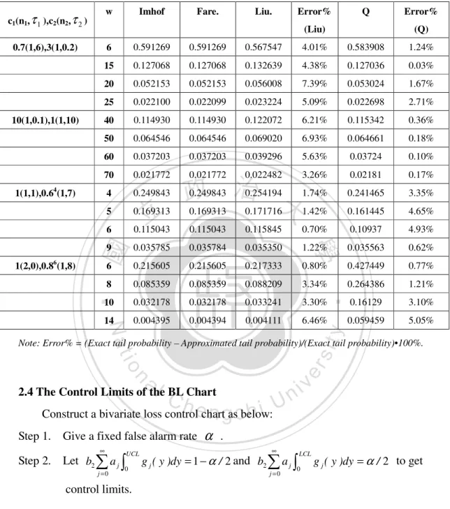
(22) •. BL ~ Ar1 χ v21 + Br2 χ v22 Step 4.. (6). Use Moschopoulos and Canada’s (1984) method to get approximated distribution of BL.. Let Q = Ar1 χ v2 + Br2 χ v2 . 1. 2. •. Thus, BL ~ Q . Step 5.. (7). From Moschopoulos and Canada (1984), the cumulative distribution function (c.d.f.) of Q is. 政治大 ∞. FQ ( q ) = P (Q ≤ q ) = b2 ∑ a j ∫ g j ( y )dy j =0. 立. q. 0. Also, a j = A(j 2) = A(c2 , j ) with A(ci , j ) =. 學. ‧ 國. where b2 = (c1 / c2 ) m2 , c1 = Ar1 , c2 = Br2 and mi = vi / 2, i = 1,2 . ( mi ) j (1 − c1 / ci ) j j!. and. ‧. g(y) is the pdf of a Gamma variable with shape parameter (m1 + m2 + j). y. Nat. and scale parameter 2c1. That is, y ~ Γ(m1 + m2 + j,2c1 ) .. er. io. sit. The approximated c.d.f. of Q is compared with Imhof (1961), Farebrother (1984), and Liu (2009) (See Table 1.). Imhof’s (1961) method shows the exact tail probability for. n. al. Ch. i n U. v. a linear combination of chi-squares. From Table 1, Farebrother’s (1984) method is. engchi. more precise, but it’s hard to calculate. Compare Liu’s (2009) method and our method, we found that our method is close to the exact value when any one of the two weights is greater than 0.2.. 12.

(23) Table 1. Compare Error% of Tail Probability P (W > w) with Imhof’s Method w. c1(n1, τ 1 ),c2(n2, τ 2 ). Liu.. Error%. Q. Error%. 0.591269. 0.591269. 0.567547. 4.01%. 0.583908. 1.24%. 15. 0.127068. 0.127068. 0.132639. 4.38%. 0.127036. 0.03%. 20. 0.052153. 0.052153. 0.056008. 7.39%. 0.053024. 1.67%. 25. 0.022100. 0.022099. 0.023224. 5.09%. 0.022698. 2.71%. 40. 0.114930. 0.114930. 0.122072. 6.21%. 0.115342. 0.36%. 50. 0.064546. 0.064546. 0.069020. 6.93%. 0.064661. 0.18%. 60. 0.037203. 0.037203. 0.039296. 5.63%. 0.03724. 0.10%. 70. 0.021772. 0.021772. 0.022482. 3.26%. 0.02181. 0.17%. 4. 0.249843. 0.249843. 0.254194. 1.74%. 0.241465. 3.35%. 5. 0.169313. 0.169313. 0.171716. 1.42%. 0.161445. 4.65%. 6. 0.115043. 0.115043. 0.115845. 0.70%. 0.10937. 4.93%. ‧ 國. (Q). 6. 9. 0.035785. 0.035784. 0.035350. 1.22%. 0.035563. 0.62%. 6. 0.215605. 0.215605. 0.217333. 0.80%. 0.427449. 0.77%. 8. 0.085359. 0.085359. 0.088209. 3.34%. 0.264386. 1.21%. 10. 0.032178. 0.032178. 0.033241. 3.30%. 0.16129. 3.10%. 14. 0.004395. 0.004394. 0.004111. 6.46%. 0.059459. 5.05%. 4. 1(1,1),0.6 (1,7). 政治大. 立. 學. 1(2,0),0.86(1,8). Fare.. (Liu). 0.7(1,6),3(1,0.2). 10(1,0.1),1(1,10). Imhof. sit. y. ‧. Nat. io. n. al. er. Note: Error% = (Exact tail probability – Approximated tail probability)/(Exact tail probability)•100%.. Ch. 2.4 The Control Limits of the BL Chart. engchi. Construct a bivariate loss control chart as below: Step 1. Give a fixed false alarm rate ∞. Step 2. Let b2 ∑ a j ∫ j =0. UCL. 0. i n U. v. α . ∞. g j ( y )dy = 1 − α / 2 and b2 ∑ a j ∫ j =0. LCL. 0. g j ( y )dy = α / 2 to get. control limits. Step 3. Since FQ (q) is the sum of an infinite sequence, we compute control limits by taking the first N terms. Thus, our control limits are approximate values. N. b2 ∑ a j ∫ j =0 N. 0. b2 ∑ a j ∫ j =0. UCL. LCL. 0. •. g j ( y )dy =1 − α / 2 ,. (8). •. g j ( y )dy = α / 2 13. (9).

(24) Hence the limits of the proposed Bivariate Loss Control Chart are •. −1. UCL = FQ (1 − α / 2) •. −1. CL = FQ ( p* ) •. −1. LCL = FQ (α / 2) N. Note that p * = b2 ∑ a j ∫ g j ( y ) dy . CL. 0. j =0. Charting procedure:. 政治大. Step 1. Specify target vector (T1, T2), mean vector µ 0 , and covariance matrix ∑ 0. 立. for in-control process. Also, set K11, K 22 and K12 .. ‧ 國 n. ‧. m. 學. Y  1 Step 2. If µ 0 is unknown, use the sample mean vector Y =   to estimate, where    Y2  Yi = ∑∑ y ijk / mn, i = 1,2 and m is the number of subgroups and n is the k =1 j =1. Nat. sit. n. al. er. m s12  s = ( s1k / c4 ) / m to to estimate it, where we use ∑ 1 s 22  k =1. io.  s2 S = 1 s  12. y. sample size. If ∑ 0 is unknown, use sample covariance matrix. m. Ch. engchi. i n U. v. estimate σ1 , s 2 = (∑ s 2 k / c 4 ) / m to estimate σ 2 and use sample correlation k =1. to estimate ρ 0 . Step 3. For each subgroup calculate BL i . Step 4. Specify our ARL0, the in-control ARL, and calculate control limits. Step 5. Plot the sample points and control limits on the chart. Step 6. If any points fall outside the control limits, i.e. BL i > UCL , BL i < LCL , then we have to stop the process and investigate the unusual causes. 2.5 The Out-of-control Approximate Distribution of BL. When process is out-of-control, 14.

(25) BL ~. 1 K K ρ 1 K2 K11 (δ 32σ 12 + ( 12 ) 2 δ 42σ 22 + 12 1 δ 3δ 4σ 12 ) χ n2,τ11 + ( K 22 − 12 )δ 42σ 22 χ n2,τ12 n 2 K11 K11 ρ 0 n 4 K11. with χ n2,τ. 11. has a non-central chi-square distribution with n degrees of freedom, and. K12 (δ 2 + δ 7 )σ 2 )2 2K11 and χ12,τ has a non-centrality parameter τ 11 = ρ K K (δ 32σ12 + ( 12 )δ 42σ 22 + 12 1 δ 3δ 4σ12 ) 2K11 K11 ρ0 n((δ1 + δ 6 )σ1 +. 12. non-central chi-square distribution with n degrees of freedom, and non-centrality parameter τ12 =. n((δ 2 + δ 7 )σ 2 ) 2. δ 42σ 22. =. n((δ 2 + δ 7 ))2. δ 42. .. 政治大. Again, we could use the same procedure as in section 1.3 to find the. 立. out-of-control approximate distribution (Q*) of BL (see 1.2). Thus, we can get that. ‧ 國. (10). ‧. K K ρ K2 1 1 K11 (δ 32σ 12 + ( 12 ) 2 δ 42σ 22 + 12 1 δ 3δ 4σ 12 ) , B' = ( K 22 − 12 )δ 42σ 22 , 4 K11 n 2 K11 K11 ρ 0 n. τ 11 τ 112 τ τ 122 and r2 ' = 1 + 12 , v2 ' = n + . , v1 ' = n + n + τ 11 n + 2τ 11 n + τ 12 n + 2τ 12. sit. y. Nat. r1 ' = 1 +. 學. where A' =. •. BL ~ Q * = A' r1 ' χ v21 ' + B' r2 ' χ v22 '. io. n. al. er. Also, by Moschopoulos and Canada (1984), we could calculate the c.d.f. of Q*.. Ch. 2.6 Performance Measurement of the BL Chart. engchi. i n U. v. We would use average run length (ARL) to measure the performance of the control charts. Define ARL1 as the average run length to signal when process is out-of-control. We give a fixed false alarm rate α . When the process is out-of-control, the power is •. 1 − β = 1 − P( LCL < BL < UCL BL ~ Q* ) −1. −1. = 1 − ( FQ* ( FQ (1 − α / 2)) − FQ* ( FQ (α / 2))) where β is the type II error when the process is out-of-control and FQ (• ) is a the *. 15.

(26) c.d.f. of Q * . Thus, ARL1 =. =. 1 1− β. 1 − ( FQ* ( FQ. −1. 1 −1 (1 − α / 2)) − FQ* ( FQ (α / 2))). (11). 2.7 Illustrating Example of the Bivariate Loss Chart. The example is taken from Yang, Lin and Hung (2009). Example:. 政治大 stability of signal transfer between the computer main hardware and its peripheral 立. The thickness of the gold film on the surface of the terminals strongly affects the. components. Also, a thin film will cause an unstable signal transfer and the terminals. ‧ 國. 學. must be re-processed or discarded. Thus, we have to control the film thickness. ‧. efficiently. 30 samples of size 4 are taken in a fixed interval from the process. For. y. Nat. each sample, we measure two related thickness from two location of a film, that is,. n. er. io. al. sit. AP-2.8 and AN-1.3. The data are listed below:. Ch. engchi. 16. i n U. v.

(27) Table 2. The data of film thickness. 政治大 Next, in order to use BL chart to monitor process, we have to check if the data 立 follow a normal distribution. Thus, we use chi-square plot (see Johnson (1992)) to. The procedure of plotting chi-square plot (or QQ-plot): Step 1.. Compute d 2j = ( y j − y )' S −1 ( y j − y ) ,. ‧. ‧ 國. 學. check.. Nat. y. j = 1, 2 , ⋯ , 120 and we rank d. er. io. Graph the pairs ( d (2j ) , χ 22 (( j − 1 / 2) / n )) , where χ 22 (( j − 1 / 2) / n ) is the. al. v i n C 100(j-1/2)/n percentile hofethe chi-square n g c h i Udistribution with 2 degrees of n. Step 2.. sit. values from small to large. j means the jth observation of the sample.. freedom. Step 3.. If any points fall near a line, we think they follow a bivariate normal distribution.. 17.

(28) 政治大. Figure 1. QQ-plot for the Film Thickness Data. 立. From Figure 1, there are some points off the line. Let’s do the test to make further. ‧ 國. 學. check the assumption.. ‧. Use Generalized Shapiro-Wilk test to test the normality.. y. Nat. H0 : The data follow a bivariate normal distribution. n. al. er. io. The result is as follows:. sit. H1 : The data do not follow a bivariate normal distribution. Ch. i n U. v. Generalized Shapiro-Wilk test for Multivariate Normality. engchi. MVW = 0.9847, p-value = 0.1486. The result shows that p-value = 0.1486 > α = 0.05 , hence we don’t have enough evident to reject the hypothesis that the data follow a bivariate normal distribution. We will now construct the BL chart to monitor the process.. 18.

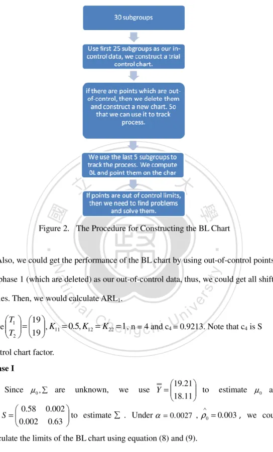
(29) 立. 政治大. ‧ 國. 學. Figure 2. The Procedure for Constructing the BL Chart. ‧. y. Nat. Also, we could get the performance of the BL chart by using out-of-control points. er. io. sit. on phase 1 (which are deleted) as our out-of-control data, thus, we could get all shift scales. Then, we would calculate ARL1.. n. al. Ch. i n U. v.  T1  19  Give   =   , K11 = 0.5, K12 = K22 = 1 , n = 4 and c4 = 0.9213. Note that c4 is S  T2  19 . engchi. control chart factor. Phase I. Since µ 0 , ∑ are. unknown,. 19.21  to use Y =  18.11. we. estimate µ 0 and. ∧  0.58 0.002   to estimate ∑ . Under α = 0.0027 , ρ 0 = 0.003 , we could use S =   0.002 0.63 . calculate the limits of the BL chart using equation (8) and (9). UCL = 4 .593. LCL = 0.244 19.

(30) For each subgroup, we compute BLi =. n 1 K 1 K2 n K11 ∑ (Y1ij − T1 + 12 (Y2ij − T2 )) 2 + ( K 22 − 12 )∑ (Y2ij − T2 ) 2 , i = 1, … ,25 n1 2 K11 n 4 K11 j =1 j =1. and plot them on the chart.. BL Co n t r o l Ch a r t 9 8 7 6 5. U CL= 4 .59 3. 4 3 2. 立. 1 0. LC L = 0 . 2 4 4 10. 15. 20. 25. s ub gro u p. Figure 3. The Trial BL Control Chart (1). ‧. ‧ 國. 5. 學. 0. 政治大. y. Nat. sit. As we could see from Figure 3, there are 5 points above the upper limit. Thus, we. al. n. control chart.. er. io. delete subgroups 19, 21, 23, 24, and 25. Then, we revise the data and construct a new. Ch. engchi. i n U. v.  0.6 0.01 19.42   to  to estimate µ 0 and use new S =  Now, we use new Y =  18.34   0.01 0.64  ∧. estimate ∑ 0 . Under α = 0.0027 , ρ 0 = 0.02 , the limits of the BL chart are: UCL = 3 .733. LCL = 0.157. 20.

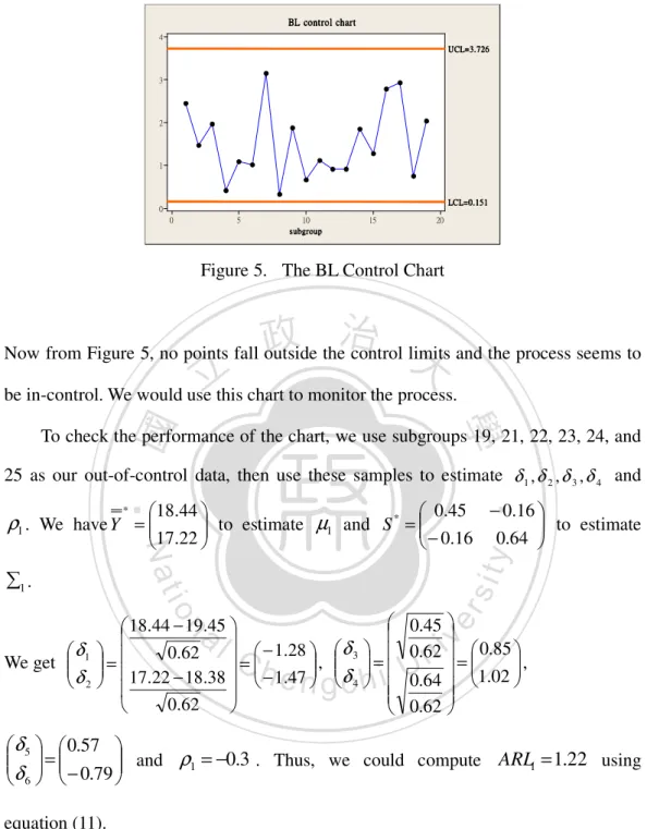
(31) BL c o n t r o l c h a r t 4 U C L= 3 . 7 3 3. 3. 2. 1. LC L = 0 . 1 5 7. 0 0. 5. 10 s u bg ro up. 15. 20. 政治大. Figure 4. The Trial BL Control Chart (2). 立. Again, we compute BL for 24 subgroups and plot them on the chart.. ‧ 國. 學. From Figure 4, we found sample 20 is above the UCL. Thus, we delete subgroup 20. ‧. (the original subgroup 22) and revise the chart.. sit. y. Nat. 19.45   0.62 0.04   to estimate µ 0 and use new S =   to We use new Y =  18.38   0.04 0.62  ∧. n. al. er. io. estimate ∑ 0 . Under α = 0.0027 , ρ 0 = 0.06 , the new limits of the BL chart are now: UCL = 3.726. Ch. engchi. LCL = 0.151. 21. i n U. v.

(32) BL co nt r o l ch ar t 4 U C L= 3 . 7 2 6. 3. 2. 1. LC L= 0 . 1 5 1. 0 0. 5. 10 s ubgroup. 15. 20. Figure 5. The BL Control Chart. 政治大. Now from Figure 5, no points fall outside the control limits and the process seems to. 立. be in-control. We would use this chart to monitor the process.. ‧ 國. 學. To check the performance of the chart, we use subgroups 19, 21, 22, 23, 24, and 25 as our out-of-control data, then use these samples to estimate δ 1 , δ 2 , δ 3 , δ 4 and. al. n.  18.44 − 19.45    δ1   0.62  =  − 1.28  , We get   =    δ 2   17.22 − 18.38   − 1.47  0.62  . Ch.   δ 3     =  δ 4    . engchi. er. io. sit. Nat. ∑1 .. − 0.16   to estimate 0.64 . y.  0.45. 18.44 . ‧. *. ρ1 . We have Y =   to estimate µ1 and S * =  17.22   − 0.16. 0.45  0.62   0.85   ,  =  0.64  1.02   0.62 . i n U. v. δ 5   0.57    =   and ρ1 = −0.3 . Thus, we could compute ARL1 = 1.22 using δ 6   − 0.79 equation (11). Phase II. With the BL chart, we track the following process. Using last 5 subgroups to track, we compute BL for each subgroup and plot them on the chart to see if the process is out-of-control.. 22.

(33) BL con tr ol char t 12 10 8 6 4. U C L= 3 .7 26. 2 L C L= 0 . 1 5 1. 0 0. 5. 10. 15. 20. 25. s u bg ro up. Figure 6. The BL Control Chart for Tracking the Process. 政治大 subgroups were outside the upper control limit. We must find cause and rectify them 立 From Figure 6, we found that the process is out-of-control since the last 5. if any. Since the BL chart couldn’t tell what caused the signal, mean vector or. ‧ 國. 學. covariance matrix. There are two methods to investigate. First, we can use in-control. ‧. data to construct T2 chart and S chart separately, then we check points on both. sit. y. Nat. charts. So, we may find out if the signal(s) came from mean vector and/or covariance. io. al. er. matrix. Second, we could compare both mean vector and covariance matrix with. v. n. in-control process through observed data directly. Two methods are illustrated below. (i). Ch. engchi. Use T2 chart and S chart to investigate.. i n U. For T2 chart, the control limits are: UCLT 2 = χ 22,1−α / 2 = 13.215 LCLT 2 = χ 22,α / 2 = 0.003. 23.

(34) For S chart, the control limits are: UCL S = χ 22n − 4,1−α / 2 = 17.8 LCL S = χ 22n − 4,α / 2 = 0.11. |S |. T2. 20 50. U C L= 1 7 . 8 15. 40. 政治大. 30. 立. 0. 6. 12 18 s ub g rou p. 5. LC L= 0 . 0 0 3. 0. 24. LC L= 0 . 1 1. 0. 6. ‧. 0. U C L= 1 3 . 1 2 5. 學. 10. ‧ 國. 20. 10. 12 18 s ub g ro up. Nat. y. 24. n. al. er. io. sit. Figure 7. Hotelling’s T2 chart and S chart. Ch. i n U. v. From Figure 7, first 19 subgroups are in-control data and the tracking data is from. engchi. subgroup 20 to 24. No point falls outside the control limits for S chart. But, we could see T2 values of subgroup 20 to 24 are outside the control limits for T2 chart. We found the mean vector has shifted from the target vector. For the subgroup 20, we could ∧   19   − 1.44 σ 1    . Also calculate the mean vector has shifted  from the target vector  ∧  − 3.32 σ 2  19    ∧    − 0.78 σ 1  we could get the mean vector of the subgroup 21 to 24 have shifted  , ∧   − 3.03σ 2   . 24.

(35) ∧    − 1.22 σ 1  ,  ∧   − 2.49 σ 2   . (ii). ∧ ∧      − 0.6 σ 1   − 1.32 σ 1  and from the target vector.   ∧  ∧   − 3.03σ 2   − 3.26 σ 2     . We calculate mean vector and covariance matrix of subgroup 20 to 24 and. 19.45   , the covariance matrix compare them with in-control mean vector  18.38   0.62 0.04    .  0.04 0.62  17.85   and the covariance matrix is 1. Subgroup 20: the mean vector is  16.43   0.51 0.05    . And we get  0.05 0.11.  δ   0.91   δ1   − 2.03    =   and  3  =   .  δ 2   − 2.48   δ 4   0.42 . 立. 2. Subgroup 21: the mean. ‧ 國. 16.65   . covariance matrix is.  δ  1.14   δ1   − 1.36    =   and  3  =   .  δ 2   − 2.2   δ 4  1.16 . 學.  0.81 0.38    . And we get  0.38 0.84 . 政 18治 .38  大  and the vector is . n. er. io. al.  δ  1.11   δ1   − 1.8    =   .  and  3  =   δ 4   0.55   δ 2   − 1.65 . sit. Nat.  0.77 − 0.13    . And we get  − 0.13 0.19 . y. ‧. 18.03   and the covariance matrix is 3. Subgroup 22: the mean vector is  17.08 . v. 18.53   and the covariance matrix is 4. Subgroup 23: the mean vector is  16.65   0.33 0.12    . And we get  0.12 0.44 . Ch. engchi. i n U.  δ   0.73   δ1   − 1.17    =   and  3  =   .  δ 2   − 2.2   δ 4   0.84 . 17.95   and the covariance matrix is 5. Subgroup 24: the mean vector is  16.48   2.83 − 0.04    . And we get  − 0.04 0.18 .  δ   2.14   δ1   − 1.91    =   and  3  =   .  δ 4   0.54   δ 2   − 2.41. As we could see that the mean vector has larger shifted than the shifts in the covariance matrix. In some subgroups, the variations decreased. We need to improve this situation. 25.

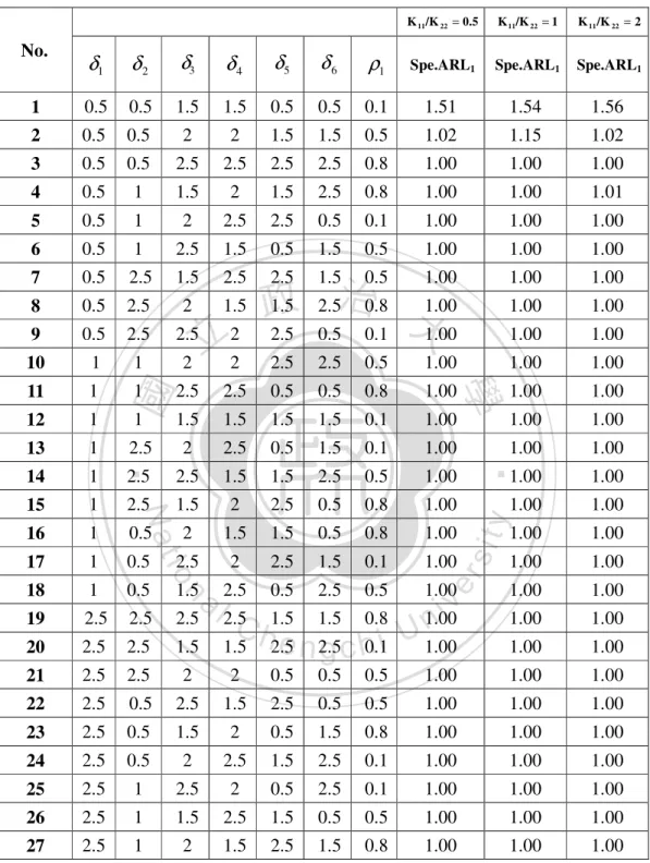
(36) Another useful approach is change point, detail of the apparach see (Hawkins et al. (2003), Hawkins and Zamba (2005) and Zamba (2006).. 2.8 ARL1 of the Bivariate Loss Chart (1). The Bivariate Loss Chart with Specified Sample Size and Sampling Interval. To investigate the impact of various combinations of δ1 , δ 2 , δ 3 , δ 4 , δ 5 , δ 6 ,. ρ1 and specified ρ 0 and K11 / K22 on ARL1, the various levels of δ1 , δ 2 , δ 3 , δ 4 ,  0. δ 5 , δ 6 , ρ1 and specified ρ0 and K11 / K22 are listed in Table 3. Set µ 0 =   ,  0. 政治大. −δ   , T =  5  and K12 = K22 = 1. 1 −δ6 . ρ0 . 立. 學. ‧ 國. 1 ∑ 0 =   ρ0. Table 3. Various levels of (δ1 , δ 2 , δ 3 , δ 4 , δ 5 , δ 6 , ρ1 ) , ρ0 and K11 / K22. δ3. δ4. δ5. δ6. ρ1. 0.5. 0.5. 1.5. 1.5. 0.5. 0.5. 0.1. 1.5. 1.5. 2. 2. 1.5. 1.5. 0.5. 2.5. 2.5. 2.5. 2.5. 2.5. 2.5. 0.8. n. Ch. The combinations of δ1 , δ 2 , δ 3 , δ 4 , δ 5 , δ 6. engchi. y. sit. er. io. al. iv n Uand ρ. ρ0. K11/K22. 0.1. 0.5. 0.5. 1. 0.8. 2. ‧. δ2. Nat. δ1. 1. are expressed under a. specified ( ρ 0 , K11 / K22). The ARL1s are calculated based on the combinations of δ1 to δ 6 and ρ1 in L27 (313) table given n = 5, α = 0.0027.. 26.

(37) Table 4. The ARL1 for Specified BL Chart Given n = 5, α = 0.0027and ρ0 = 0.1. No.. K 11 /K 22 = 0.5. K 11/K 22 = 1. K 11 /K 22 = 2. δ1. δ2. δ3. δ4. δ5. δ6. ρ1. Spe.ARL1. Spe.ARL1. Spe.ARL1. 1. 0.5. 0.5. 1.5. 1.5. 0.5. 0.5. 0.1. 1.51. 1.54. 1.56. 2. 0.5. 0.5. 2. 2. 1.5. 1.5. 0.5. 1.02. 1.15. 1.02. 3. 0.5. 0.5. 2.5. 2.5. 2.5. 2.5. 0.8. 1.00. 1.00. 1.00. 4. 0.5. 1. 1.5. 2. 1.5. 2.5. 0.8. 1.00. 1.00. 1.01. 5. 0.5. 1. 2. 2.5. 2.5. 0.5. 0.1. 1.00. 1.00. 1.00. 6. 0.5. 1. 2.5. 1.5. 0.5. 1.5. 0.5. 1.00. 1.00. 1.00. 7. 0.5. 2.5. 1.5. 2.5. 2.5. 1.5. 0.5. 1.00. 1.00. 1.00. 8. 0.5. 2.5. 2. 1.5. 1.00. 1.00. 9. 0.5. 2.5. 2.5. 1.00. 1.00. 10. 1. 1. 1.00. 1.00. 11. 1. 12. 1. 13. 1. 14. 1. 15. 2.5. 2.5. 0.5. 1.00. 學. 2.5. 2.5. 0.5. 0.5. 0.8. 1.00. 1.00. 1.00. 1. 1.5. 1.5. 1.5. 1.5. 0.1. 1.00. 1.00. 1.00. 2.5. 2. 2.5. 0.5. 1.5. 0.1. 1.00. 1.00. 1.00. 2.5. 2.5. 1.5. 1.5. 2.5. 0.5. 1.00. 1.00. 1.00. 1. 2.5. 1.5. 2. 2.5. 0.5. 0.8. 1.00. 1.00. 1.00. 16. 1. 0.5. 2. 1.5. 1.5. 0.5. 0.8. 1.00. 1.00. 1.00. 17. 1. 0.5. 2.5. 2. 2.5. 1.5. 0.1. 1.00. 1.00. 1.00. 18. 1. 0.5. 1.00. 1.00. 19. 2.5. 2.5. 1.00. 1.00. 20. 2.5. 2.5. 1.00. 1.00. 21. 2.5. 2.5. 2. 2. 0.5. 0.5. 0.5. 1.00. 1.00. 1.00. 22. 2.5. 0.5. 2.5. 1.5. 2.5. 0.5. 0.5. 1.00. 1.00. 1.00. 23. 2.5. 0.5. 1.5. 2. 0.5. 1.5. 0.8. 1.00. 1.00. 1.00. 24. 2.5. 0.5. 2. 2.5. 1.5. 2.5. 0.1. 1.00. 1.00. 1.00. 25. 2.5. 1. 2.5. 2. 0.5. 2.5. 0.1. 1.00. 1.00. 1.00. 26. 2.5. 1. 1.5. 2.5. 1.5. 0.5. 0.5. 1.00. 1.00. 1.00. 27. 2.5. 1. 2. 1.5. 2.5. 1.5. 0.8. 1.00. 1.00. 1.00. er. io. sit. y. ‧. 1. Nat. ‧ 國. 2 立 2 2. 1.5 2.5治 0.8 1.00 政大 2.5 0.5 0.1 1.00. a l 2.5 0.5 2.5 0.5 1.00i v 2.5 2.5 n C h1.5 1.5 0.8 U 1.00 i e n 2.5 1.5 1.5 2.5 g c h0.1 1.00 n. 1.5. 27.

(38) Table 5. The ARL1 for Specified BL Chart Given n = 5, α = 0.0027and ρ0 = 0.5 K 11/K 22 = 1. K 11 /K 22 = 2. δ1. δ2. δ3. δ4. δ5. δ6. ρ1. Spe.ARL1. Spe.ARL1. Spe.ARL1. 1. 0.5. 0.5. 1.5. 1.5. 0.5. 0.5. 0.1. 1.39. 2.03. 1.45. 2. 0.5. 0.5. 2. 2. 1.5. 1.5. 0.5. 1.01. 1.06. 1.01. 3. 0.5. 0.5. 2.5. 2.5. 2.5. 2.5. 0.8. 1.00. 1.00. 1.00. 4. 0.5. 1. 1.5. 2. 1.5. 2.5. 0.8. 1.00. 1.01. 1.01. 5. 0.5. 1. 2. 2.5. 2.5. 0.5. 0.1. 1.00. 1.00. 1.00. 6. 0.5. 1. 2.5. 1.5. 0.5. 1.5. 0.5. 1.00. 1.00. 1.00. 7. 0.5. 2.5. 1.5. 2.5. 1.00. 1.00. 8. 0.5. 2.5. 1.00. 1.00. 9. 0.5. 2.5. 1.5 立 2.5 2. 1.00. 1.00. 10. 1. 11. 1. 12. 1. 13. 1. ‧ 國. No.. K 11 /K 22 = 0.5. 14. 2. 2.5 1.5治 0.5 1.00 政大 1.5 2.5 0.8 1.00 2.5. 0.5. 0.1. 1.00. 2.5. 2.5. 0.5. 1.00. 1.00. 1.00. 1. 2.5. 2.5. 0.5. 0.5. 0.8. 1.00. 1.00. 1.00. 1. 1.5. 1.5. 1.5. 1.5. 0.1. 1.00. 1.00. 1.00. 2.5. 2. 2.5. 0.5. 1.5. 0.1. 1.00. 1.00. 1.00. 1. 2.5. 2.5. 1.5. 1.5. 2.5. 0.5. 1.00. 1.00. 1.00. 15. 1. 2.5. 1.5. 2. 2.5. 0.5. 0.8. 1.00. 1.00. 1.00. 16. 1. 0.5. 2. 1.5. 1.5. 0.5. 0.8. 1.00. 1.00. 1.00. 17. 1. 0.5. 2.5. 2. 2.5. 1.5. 0.1. 1.00. 1.00. 1.00. 18. 1. 0.5. 1.5. 2.5. 1.00. 1.00. 19. 2.5. 2.5. 2.5. C h0.5 2.5 0.5 U e n 1.5 2.5 1.5 g c h0.8i 1.00. 1.00. 1.00. 20. 2.5. 2.5. 1.5. 1.5. 2.5. 2.5. 0.1. 1.00. 1.00. 1.00. 21. 2.5. 2.5. 2. 2. 0.5. 0.5. 0.5. 1.00. 1.00. 1.00. 22. 2.5. 0.5. 2.5. 1.5. 2.5. 0.5. 0.5. 1.00. 1.00. 1.00. 23. 2.5. 0.5. 1.5. 2. 0.5. 1.5. 0.8. 1.00. 1.00. 1.00. 24. 2.5. 0.5. 2. 2.5. 1.5. 2.5. 0.1. 1.00. 1.00. 1.00. 25. 2.5. 1. 2.5. 2. 0.5. 2.5. 0.1. 1.00. 1.00. 1.00. 26. 2.5. 1. 1.5. 2.5. 1.5. 0.5. 0.5. 1.00. 1.00. 1.00. 27. 2.5. 1. 2. 1.5. 2.5. 1.5. 0.8. 1.00. 1.00. 1.00. 28. y. sit. er. io. al. ‧. 2. n. 學. 2. Nat. 1. v 1.00 ni.

(39) Table 6. The ARL1 for Specified BL Chart Given n = 5, α = 0.0027and ρ 0 = 0.8 K 11/K 22 = 1. K 11 /K 22 = 2. δ1. δ2. δ3. δ4. δ5. δ6. ρ1. Spe.ARL1. Spe.ARL1. Spe.ARL1. 1. 0.5. 0.5. 1.5. 1.5. 0.5. 0.5. 0.1. 1.31. 2.00. 1.39. 2. 0.5. 0.5. 2. 2. 1.5. 1.5. 0.5. 1.00. 1.03. 1.01. 3. 0.5. 0.5. 2.5. 2.5. 2.5. 2.5. 0.8. 1.00. 1.00. 1.00. 4. 0.5. 1. 1.5. 2. 1.5. 2.5. 0.8. 1.00. 1.01. 1.01. 5. 0.5. 1. 2. 2.5. 2.5. 0.5. 0.1. 1.00. 1.00. 1.00. 6. 0.5. 1. 2.5. 1.5. 0.5. 1.5. 0.5. 1.00. 1.00. 1.00. 7. 0.5. 2.5. 1.5. 2.5. 1.00. 1.00. 8. 0.5. 2.5. 1.00. 1.00. 9. 0.5. 2.5. 1.5 立 2.5 2. 1.00. 1.00. 10. 1. 11. 1. 12. 1. 13. 1. ‧ 國. No.. K 11 /K 22 = 0.5. 14. 2. 2.5 1.5治 0.5 1.00 政大 1.5 2.5 0.8 1.00 2.5. 0.5. 0.1. 1.00. 2.5. 2.5. 0.5. 1.00. 1.00. 1.00. 1. 2.5. 2.5. 0.5. 0.5. 0.8. 1.00. 1.00. 1.00. 1. 1.5. 1.5. 1.5. 1.5. 0.1. 1.00. 1.00. 1.00. 2.5. 2. 2.5. 0.5. 1.5. 0.1. 1.00. 1.00. 1.00. 1. 2.5. 2.5. 1.5. 1.5. 2.5. 0.5. 1.00. 1.00. 1.00. 15. 1. 2.5. 1.5. 2. 2.5. 0.5. 0.8. 1.00. 1.00. 1.00. 16. 1. 0.5. 2. 1.5. 1.5. 0.5. 0.8. 1.00. 1.00. 1.00. 17. 1. 0.5. 2.5. 2. 2.5. 1.5. 0.1. 1.00. 1.00. 1.00. 18. 1. 0.5. 1.5. 2.5. 1.00. 1.00. 19. 2.5. 2.5. 2.5. C h0.5 2.5 0.5 U e n 1.5 2.5 1.5 g c h0.8i 1.00. 1.00. 1.00. 20. 2.5. 2.5. 1.5. 1.5. 2.5. 2.5. 0.1. 1.00. 1.00. 1.00. 21. 2.5. 2.5. 2. 2. 0.5. 0.5. 0.5. 1.00. 1.00. 1.00. 22. 2.5. 0.5. 2.5. 1.5. 2.5. 0.5. 0.5. 1.00. 1.00. 1.00. 23. 2.5. 0.5. 1.5. 2. 0.5. 1.5. 0.8. 1.00. 1.00. 1.00. 24. 2.5. 0.5. 2. 2.5. 1.5. 2.5. 0.1. 1.00. 1.00. 1.00. 25. 2.5. 1. 2.5. 2. 0.5. 2.5. 0.1. 1.00. 1.00. 1.00. 26. 2.5. 1. 1.5. 2.5. 1.5. 0.5. 0.5. 1.00. 1.00. 1.00. 27. 2.5. 1. 2. 1.5. 2.5. 1.5. 0.8. 1.00. 1.00. 1.00. 29. y. sit. er. io. al. ‧. 2. n. 學. 2. Nat. 1. v 1.00 ni.

(40) From Table 4 to Table 6, we found out that no matter what the correlation between the two quality characteristics is when the process is in-control, the specified BL chart is insensitive to larger process shifts. And the ratio of K11 / K22 hardly affects the performance, since their ARL1 is near 1 for δ1 , δ 2 ≥ 0.5 , δ 3 , δ 4 ≥ 2 ,. δ 6 , δ 7 ≥ 1.5 . Also, we found that the specified BL chart is insensitive to ρ1 when the process has large shifted. 2.. To investigate the performance of the BL chart for small shifts, we consider the. 政治大. following combinations of δ1 , δ 2 , δ 3 , δ 4 , δ 5 , δ 6 and ρ1 . Also, we calculate. 立. ARL1 under specified K11 / K22 = 0.5, 1, 2, 4 and ρ 0 = 0.1, 0.5, 0.8 given n = 5 and. ‧ 國. 學. α = 0.0027.. ‧. Table 7. Various levels of (δ1 , δ 2 , δ 3 , δ 4 , δ 5 , δ 6 , ρ1 ). δ4. δ6. δ7. y. ρ1. 0.1. 1.1. 1.1. 0.1. 0.1. sit. 0.1. 0.5. 0.5. 1.5. 0.5. 0.5. 1. 1. a l 1.5 2C h. 2. 1. 0.1. io. δ3. er. Nat δ2. δ1. n. engchi U. 30. 0.5. v ni 1. 0.8.

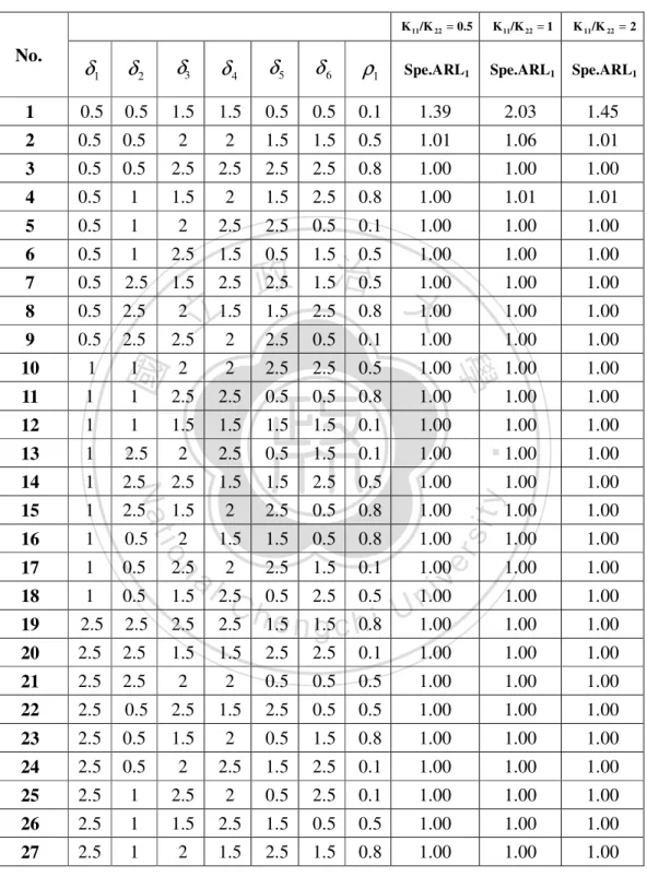
(41) Table 8. The ARL1 for Specified BL Chart of Small Shifts Given n = 5, α = 0.0027 and ρ0 = 0.5 K 11 /K 22 = 0.5. No.. δ1. δ2. δ3 δ 4 δ 5 δ 6 ρ1. K 11/K 22 = 1. K 11 /K 22 = 2. K 11 /K 22 = 4. Spe.ARL1. Spe.ARL1. Spe.ARL1. Spe.ARL1. 1. 0.1 0.1 1.1 1.1 0.1 0.1 0.1. 132.97. 391.00. 67.14. 4.54. 2. 0.1 0.1 1.5 1.5 0.5 0.5 0.5. 15.63. 76.42. 18.14. 2.94. 3. 0.1 0.1. 1. 1. 0.8. 4.58. 23.02. 5.99. 1.74. 4. 0.1 0.5 1.1 1.5 0.5. 1. 0.8. 1.92. 2.93. 2.33. 1.34. 5. 0.1 0.5 1.5. 1 0.1 0.1. 1.89. 3.79. 2.31. 1.28. 6. 0.1 0.5. 1.1 0.1 0.5 0.5. 1.38. 1.07. 7. 0.1. 1. 1.1. 1.21. 1.05. 8. 0.1. 1. 1.5. 1 立 1.1 0.5. 9. 0.1. 1. 2. 1.5. 1. 10. 0.5 0.5 1.5 1.5. 1. 11. 0.5 0.5. 2. 2. 2. 2 2. 1.18 1.88 政治大 0.5 0.5 1.10 1.25 1.11. 1.09. 1.03. 0.1 0.1. 1.00. 1.03. 1.02. 1.00. 0.5. 1.48. 1.71. 1.87. 1.21. 0.1 0.1 0.8. 1.16. 1.43. 1.40. 1.09. 12. 0.5 0.5 1.1 1.1 0.5 0.5 0.1. 1.17. 1.23. 1.05. 1.00. 13. 0.5. 1. 1.5. 2.32. 2.06. 1.71. 1.13. 14. 0.5. 1. 2. 0.5. 1.31. 1.48. 2.40. 1.04. 15. 0.5. 1. 0.1 0.8. 1.08. 1.08. 1.01. 1.00. 16. 0.5 0.1 1.5 1.1 0.5 0.1 0.8. 1.32. 1.80. 2.64. 1.49. 17. 0.5 0.1. iv n1.69. 2.01. 1.23. 18. 0.5 0.1 1.1. 1.30. 1.13. 1.02. 1.20. 1.17. 1.13. 1.03. 1.1 0.5. io. 1.1 1.5. 1. 1. n. al. 2 2. 1.5 2. 19. 1. 1. 20. 1. 1. 1.1 1.1. 0.1. 1.13. 1.11. 1.01. 1.00. 21. 1. 1. 1.5 1.5 0.1 0.1 0.5. 1.02. 1.02. 1.00. 1.00. 22. 1. 0.1. 0.1 0.5. 1.09. 1.22. 1.46. 1.20. 23. 1. 0.1 1.1 1.5 0.1 0.5 0.8. 1.12. 1.32. 1.13. 1.02. 24. 1. 0.1 1.5. 25. 1. 0.5. 26. 1. 0.5 1.1. 27. 1. 0.5 1.5 1.1. 2. 2. 2. C0.5h 0.1 1.08 U e n g 1.09 0.1 1 0.5 chi 1. 1.1 2. 0.5 0.5 0.8. y. 0.1 0.5 0.1. sit. Nat. 2. er. 2. 1. ‧. ‧ 國. 1.02. 學. 0.8. 2. 1. 1 1. 1. 0.5. 1. 0.1. 1.03. 1.12. 1.03. 1.00. 1.5 0.1. 1. 0.1. 1.20. 1.25. 1.29. 1.07. 0.5 0.1 0.5. 1.11. 1.21. 1.05. 1.00. 1.01. 1.04. 1.00. 1.00. 2. 1. 0.5 0.8. 31.

(42) Table 8 shows that there are unreasonable ARL1 with δ1 , δ 2 = 0.1, δ 3 , δ 4 = 1.1, δ 5 , δ 6 = 0.1, ρ1 = 0.1 under ρ0 = 0.5 . We also did the analysis under ρ0 = 0.1, 0.8 (See Appendix B, Table 49 and Table 50.). When ρ0 = 0.8 , we saw the same problem as ρ0 = 0.5 . Next, we calculate ARL1 under some combinations of δ1 , δ 2 , δ 3 , δ 4 , δ 5 ,. δ 6 and ρ1 . The results are shown in Table 9. Table 9.. ‧ 國. 1. 0.1. 0.1. 0.1. ρ1 Spe. ARL1. δ6. 1.05 1.05. 0.1. 0.1. 0.1. 0.1. 1.1. 1.1. 0.1. 0.1. 0.1. 0.1. 0.1. 1.2. 1.1. 0.1. 0.1. 0.1. 0.1. 0.1. 1.1. 1.2. 0.1. 0.1. 0.1. 5. 0.1. 0.1. 1.2. 1.2. 0.1. 0.1. 0.1. 125.36. 6. 0.1. 0.1. 1.1. 1.1. 0.1. 0.1. 0.2. 284.08. 7. 0.1. 1.2. 1.2. 0.1. n. a0.1l. From Table 9, we have. Ch. engchi. 195.36. y. 4. 391.00 260.52. sit. 3. 506.56. ‧. 2. io. δ5. 1. δ3. δ4. er. δ2. Nat. δ1. 學. No.. 政治大 Reasonable ARL under Small Shifts of process Parameters 立. 0.1 0.2 iv n U. 86.54. 1. Change δ 3 from 1.1 to 1.2, then ARL1 becomes reasonable. 2. Change δ4 from 1.1 to 1.2, then ARL1 becomes reasonable. 3. Change ρ1 from 0.1 to 0.2, then ARL1 becomes reasonable. 4. Compare to δ4 and ρ1 , changing δ 3 has more effect on ARL1. We found that when the shift scales of (δ 3 , δ 4 , ρ1 ) is small, ( δ 3 , δ 4 = 1.1, ρ1 = 0.1), ARL1 gets bigger than ARL0 = 370. To have a reasonable ARL1, at least one δ 3 , 32.

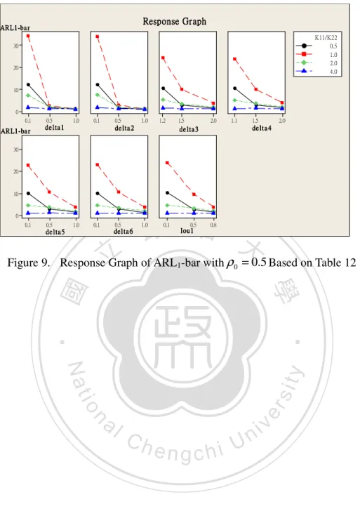
(43) δ 4 ≥ 1.2 or ρ1 ≥ 0.2 . So, for the following ARL1 analysis we will change δ3 = 1.1 to δ 3 = 1.2 . We change δ3 = 1.1 to δ3 = 1.2 in Table 7 and calculate ARL1 with specified K11/K22 = 0.5, 1, 2, 4 and ρ0 = 0.1, 0.5, 0.8 based on the various combinations of. δ1 , δ 2 , δ 3 , δ 4 , δ 5 , δ 6 and ρ1 (See Table 10.). The results are shown in Table 11- 13. Also, we drew the response graph of ARL1 – bar (See Figure 8 – 10.) based on each table.. 政治大 Table 10. Various levels of (δ , δ , δ , δ , δ , δ , ρ ) 立 1. 6. 1. δ3. δ4. δ5. δ6. ρ1. 0.1. 1.2. 1.1. 0.1. 0.1. 0.1. 0.5. 1.5. 1.5. 0.5. 0.5. 0.5. 1. 2. 2. 1. 1. 0.8. io. sit. y. Nat. n. al. er. 1. 5. ‧. 0.5. 4. δ2. ‧ 國. 0.1. 3. 學. δ1. 2. Ch. engchi. 33. i n U. v.

(44) Table 11. The ARL1 for Specified BL Chart of Small Shifts Given n = 5,. α = 0.0027 and ρ0 = 0.1. No.. δ1. δ2. K 11 /K 22 = 0.5. K 11 /K 22 = 1. K 11 /K 22 = 2. K 11 /K 22 = 4. Spe.ARL1. Spe.ARL1. Spe.ARL1. Spe.ARL1. δ3 δ 4 δ 5 δ 6 ρ1. 1. 0.1 0.1 1.2 1.1 0.1 0.1 0.1. 59.31. 47.16. 40.06. 3.36. 2. 0.1 0.1 1.5 1.5 0.5 0.5 0.5. 2.70. 2.81. 2.84. 1.35. 3. 0.1 0.1. 1. 1. 0.8. 1.12. 1.19. 1.12. 1.02. 4. 0.1 0.5 1.2 1.5 0.5. 1. 0.8. 1.83. 2.38. 4.02. 1.79. 5. 0.1 0.5 1.5. 1 0.1 0.1. 1.18. 1.43. 1.14. 1.02. 6. 0.1 0.5. 1.1 0.1 0.5 0.5. 1.85. 1.25. 7. 0.1. 1. 1.2. 1.17. 1.05. 8. 0.1. 1. 1.5. 1 立 1.1 0.5. 9. 0.1. 1. 2. 1.5. 1. 10. 0.5 0.5 1.5 1.5. 1. 11. 0.5 0.5. 2. 2. 2 2 2. 2.00 1.82 政治大 0.5 0.5 1.03 1.23 1.61. 2.09. 1.28. 0.1 0.1. 1.05. 1.12. 1.03. 1.00. 0.5. 1.15. 1.27. 1.15. 1.01. 0.1 0.1 0.8. 1.09. 1.10. 1.15. 1.03. 12. 0.5 0.5 1.2 1.1 0.5 0.5 0.1. 3.61. 3.78. 3.63. 1.35. 13. 0.5. 1. 1.03. 1.08. 1.26. 1.12. 14. 0.5. 1. 0.5. 1.09. 1.09. 1.12. 1.02. 15. 0.5. 1. 0.1 0.8. 1.10. 1.30. 1.10. 1.01. 16. 0.5 0.1 1.5 1.1 0.5 0.1 0.8. 2.42. 2.15. 1.61. 1.10. 17. 0.5 0.1. iv n1.16. 1.02. 1.00. 18. 0.5 0.1 1.2. 1.58. 2.15. 1.85. 1.00. 1.00. 1.00. 1.00. 1.1 0.5. io. 1.2 1.5. 1. n. al. 1. 2 2. 1.5 2. 19. 1. 1. 20. 1. 1. 1.2 1.1. 0.1. 1.05. 1.12. 1.06. 1.00. 21. 1. 1. 1.5 1.5 0.1 0.1 0.5. 1.09. 1.10. 1.17. 1.02. 22. 1. 0.1. 0.1 0.5. 1.05. 1.02. 1.00. 1.00. 23. 1. 0.1 1.2 1.5 0.1 0.5 0.8. 1.71. 1.70. 1.93. 1.26. 24. 1. 0.1 1.5. 25. 1. 0.5. 26. 1. 0.5 1.2. 27. 1. 0.5 1.5 1.1. 2. 2. 2. 0.1 1.15 C 0.5 0.1 h 1 e0.5 hi U n g c1.37 1. 1.1 2. 0.5 0.5 0.8. y. 0.1 0.5 0.1. sit. 2. 2. er. Nat. 1.5. 2. 1. ‧. ‧ 國. 1.45. 學. 0.8. 2. 1. 1 1. 1. 0.5. 1. 0.1. 1.10. 1.09. 1.11. 1.01. 1.5 0.1. 1. 0.1. 1.05. 1.05. 1.05. 1.02. 0.5 0.1 0.5. 1.14. 1.16. 1.12. 1.01. 1.10. 1.13. 1.02. 1.00. 2. 1. 0.5 0.8. 34.

(45) R e sp o n s e G r a p h. A R L1 _ba r 8. K11/K22 0.5 1.0 2.0 4.0. 6 4 2 0 0.1 A R L1_ ba r. 0.5 de lta 1. 1.0. 0.1. 0.5 de lta 2. 1.0. 0.5 de lta 5. 1.0. 0.1. 0.5 d e lta 6. 1.0. 1.2. 1.5 d e lta 3. 2.0. 1.1. 1.5 de lta 4. 2.0. 8 6 4. 2 0 0.1. 0.1. 0.5 lou 1. 0.8. 政治大. Figure 8. Response Graph of ARL1-bar with ρ0 = 0.1 Based on Table 11. 立. ‧. ‧ 國. 學. n. er. io. sit. y. Nat. al. Ch. engchi. 35. i n U. v.

(46) Table 12. The ARL1 for Specified BL Chart of Small Shifts Given n = 5,. α = 0.0027 and ρ0 = 0.5. No.. δ1. δ2. K 11 /K 22 = 0.5. K 11 /K 22 = 1. K 11 /K 22 = 2. K 11 /K 22 = 4. Spe.ARL1. Spe.ARL1. Spe.ARL1. Spe.ARL1. δ3 δ 4 δ 5 δ 6 ρ1. 1. 0.1 0.1 1.2 1.1 0.1 0.1 0.1. 82.37. 195.36. 30.62. 3.20. 2. 0.1 0.1 1.5 1.5 0.5 0.5 0.5. 15.63. 76.42. 18.14. 2.94. 3. 0.1 0.1. 1. 1. 0.8. 4.58. 23.02. 5.99. 1.74. 4. 0.1 0.5 1.2 1.5 0.5. 1. 0.8. 1.62. 3.47. 3.98. 1.73. 5. 0.1 0.5 1.5. 1 0.1 0.1. 1.89. 3.79. 2.31. 1.28. 6. 0.1 0.5. 1.1 0.1 0.5 0.5. 1.38. 1.07. 7. 0.1. 1. 1.2. 1.13. 1.04. 8. 0.1. 1. 1.5. 1 立 1.1 0.5. 9. 0.1. 1. 2. 1.5. 1. 10. 0.5 0.5 1.5 1.5. 1. 11. 0.5 0.5. 2. 2. 2 2 2. 1.18 1.88 政治大 0.5 0.5 1.02 1.17 1.11. 1.09. 1.03. 0.1 0.1. 1.00. 1.03. 1.02. 1.00. 0.5. 1.48. 1.71. 1.87. 1.21. 0.1 0.1 0.8. 1.16. 1.43. 1.40. 1.09. 12. 0.5 0.5 1.2 1.1 0.5 0.5 0.1. 3.85. 9.61. 3.42. 1.36. 13. 0.5. 1. 2.32. 2.06. 1.71. 1.13. 14. 0.5. 1. 0.5. 1.31. 1.48. 2.40. 1.04. 15. 0.5. 1. 0.1 0.8. 1.06. 1.20. 1.08. 1.01. 16. 0.5 0.1 1.5 1.1 0.5 0.1 0.8. 1.32. 1.80. 2.64. 1.49. 17. 0.5 0.1. iv n1.69. 2.01. 1.23. 18. 0.5 0.1 1.2. 2.01. 2.79. 1.76. 1.20. 1.17. 1.13. 1.03. 1.1 0.5. io. 1.2 1.5. 1. n. al. 1. 2 2. 1.5 2. 19. 1. 1. 20. 1. 1. 1.2 1.1. 0.1. 1.02. 1.23. 1.04. 1.00. 21. 1. 1. 1.5 1.5 0.1 0.1 0.5. 1.02. 1.02. 1.00. 1.00. 22. 1. 0.1. 0.1 0.5. 1.09. 1.22. 1.46. 1.20. 23. 1. 0.1 1.2 1.5 0.1 0.5 0.8. 2.05. 2.34. 2.32. 1.24. 24. 1. 0.1 1.5. 25. 1. 0.5. 26. 1. 0.5 1.2. 27. 1. 0.5 1.5 1.1. 2. 2. 2. 0.1 1.08 C 0.5 0.1 h 1 e0.5 hi U n g c1.52 1. 1.1 2. 0.5 0.5 0.8. y. 0.1 0.5 0.1. sit. 2. 2. er. Nat. 1.5. 2. 1. ‧. ‧ 國. 1.02. 學. 0.8. 2. 1. 1 1. 1. 0.5. 1. 0.1. 1.03. 1.12. 1.03. 1.00. 1.5 0.1. 1. 0.1. 1.20. 1.25. 1.29. 1.07. 0.5 0.1 0.5. 1.11. 1.27. 1.09. 1.01. 1.01. 1.04. 1.00. 1.00. 2. 1. 0.5 0.8. 36.

(47) Resp o n se G r a p h. AR L 1 -b a r. K11/K22 0.5 1.0 2.0 4.0. 30. 20. 10. 0 0.1. AR L1 - b a r. 0.5. 1.0. 0.1. 0.5. de lta 1. 1.0. 1.2. de lta 2. 1.5. 2.0. 1.1. 1.5. 2.0. de lt a 4. de lta 3. 30. 20. 10. 0 0.1. 0.5. 1.0. 0.1. 0.5. 立. 政治大. 1.0. de l ta 6. de lta 5. 0.1. 0.5. lou1. 0.8. Figure 9. Response Graph of ARL1-bar with ρ 0 = 0.5 Based on Table 12. ‧. ‧ 國. 學. n. er. io. sit. y. Nat. al. Ch. engchi. 37. i n U. v.

(48) Table 13. The ARL1 for Specified BL Chart of Small Shifts Given n = 5,. α = 0.0027 and ρ 0 = 0.8. No.. δ1. δ2. K 11 /K 22 = 0.5. K 11 /K 22 = 1. K 11 /K 22 = 2. K 11 /K 22 = 4. Spe.ARL1. Spe.ARL1. Spe.ARL1. Spe.ARL1. δ3 δ 4 δ 5 δ 6 ρ1. 1. 0.1 0.1 1.2 1.1 0.1 0.1 0.1. 52.50. 254.84. 24.46. 3.11. 2. 0.1 0.1 1.5 1.5 0.5 0.5 0.5. 11.87. 71.89. 15.11. 2.87. 3. 0.1 0.1. 1. 1. 0.8. 3.65. 14.64. 5.09. 1.70. 4. 0.1 0.5 1.2 1.5 0.5. 1. 0.8. 1.47. 4.30. 3.48. 1.69. 5. 0.1 0.5 1.5. 1 0.1 0.1. 1.72. 3.70. 2.15. 1.27. 6. 0.1 0.5. 1.1 0.1 0.5 0.5. 1.32. 1.07. 7. 0.1. 1. 1.2. 1.12. 1.04. 8. 0.1. 1. 1.5. 1 立 1.1 0.5. 9. 0.1. 1. 2. 1.5. 1. 10. 0.5 0.5 1.5 1.5. 1. 11. 0.5 0.5. 2. 2. 2 2 2. 1.13 1.64 政治大 0.5 0.5 1.01 1.13 1.11. 1.08. 1.02. 0.1 0.1. 1.00. 1.02. 1.02. 1.00. 0.5. 1.38. 2.08. 1.78. 1.20. 0.1 0.1 0.8. 1.12. 1.54. 1.34. 1.08. 12. 0.5 0.5 1.2 1.1 0.5 0.5 0.1. 3.19. 9.25. 3.08. 1.35. 13. 0.5. 1. 2.05. 2.59. 1.63. 1.12. 14. 0.5. 1. 0.5. 1.23. 1.79. 1.30. 1.04. 15. 0.5. 1. 0.1 0.8. 1.05. 1.16. 1.07. 1.01. 16. 0.5 0.1 1.5 1.1 0.5 0.1 0.8. 1.24. 2.30. 2.43. 1.46. 17. 0.5 0.1. iv n1.97. 1.82. 1.21. 18. 0.5 0.1 1.2. 2.49. 3.36. 1.71. 1.16. 1.24. 1.17. 1.03. 1.1 0.5. io. 1.2 1.5. 1. n. al. 1. 2 2. 1.5 2. 19. 1. 1. 20. 1. 1. 1.2 1.1. 0.1. 1.01. 1.14. 1.03. 1.00. 21. 1. 1. 1.5 1.5 0.1 0.1 0.5. 1.01. 1.01. 1.00. 1.00. 22. 1. 0.1. 0.1 0.5. 1.06. 1.34. 1.61. 1.18. 23. 1. 0.1 1.2 1.5 0.1 0.5 0.8. 1.84. 3.11. 2.17. 1.23. 24. 1. 0.1 1.5. 25. 1. 0.5. 26. 1. 0.5 1.2. 27. 1. 0.5 1.5 1.1. 2. 2. 2. 0.1 1.06 C 0.5 0.1 h 1 e0.5 hi U n g c1.40 1. 1.1 2. 0.5 0.5 0.8. y. 0.1 0.5 0.1. sit. 2. 2. er. Nat. 1.5. 2. 1. ‧. ‧ 國. 1.02. 學. 0.8. 2. 1. 1 1. 1. 0.5. 1. 0.1. 1.02. 1.08. 1.02. 1.00. 1.5 0.1. 1. 0.1. 1.14. 1.42. 1.40. 1.07. 0.5 0.1 0.5. 1.08. 1.22. 1.08. 1.01. 1.01. 1.03. 1.00. 1.00. 2. 1. 0.5 0.8. 38.