非常態間斷隨機變數的產生 - 政大學術集成

全文

(1)國立政治大學心理學系碩士論文 Master Thesis of Department of Psychology, National Chengchi University 指導教授：鄭中平博士 Advisor：Dr. Chung-Ping Cheng. 立. 政治大. ‧ 國. 學. 非常態間斷隨機變數的產生 Generation of Non-Normal Approximated. ‧. n. al. er. io. sit. y. Nat. Discrete Random Variables. Ch. engchi. i n U. v. 碩士生：李晏撰 Graduate Student: Yen Lee 中華民國九十九年七月 July, 2010.

(2) 摘要使用母數統計方法（Parametric Tests）分析資料時，常需滿足常態假設，但實際得到的資料卻少有常態，因此研究違反常態假設對統計量所造成影響的強韌性研究（Robustness Research）在應用統計方法上是重要的研究主題。在進行此類研究時，常使用蒙地卡羅法（Monte Carlo Method）產生非常態之資料進一步進行研究，目前雖已有多個可產生非常態連續資料的方法被提出，但心理學研究之資. 政治大. 料卻多為間斷資料。而在產生非常態間斷資料時，除難以產生指定參數之間斷分. 立. 配外，亦有無限多組具同樣參數之間斷分配可供選擇。針對以上兩困難，本研究. ‧ 國. 學. 提出可使用最大資訊熵程序估計符合指定參數之單變數間斷分配，用以產生對應. ‧. 之單變數間斷資料。最大資訊熵方法可所估出之間斷最大資訊熵分配除為符合指. Nat. io. sit. y. 定參數時最常出現之分配以外，同時具有平滑、非必要無 0 機率等特性。本研究. er. 呈現指定 4 參數（平均數、變異數、偏態及峰度）與指定 2 參數（偏態及峰度）. al. n. v i n C hR 套件，並以 R 套件對此之最大資訊熵方法，及相對應之 2 方法進行探討評估。 engchi U 結果發現本研究所提出之二方法，在要求指定參數與估計參數之誤差均不超過 .001 時，均可估計出符合指定參數之可能組合之分配，顯示此二方法可精確產生指定參數之間斷分配。而本研究所提供之 R 套件，除可在輸入點數、指定參數後產生間斷分配，亦可輸入指定樣本數目及樣本數於此間斷分配中抽取樣本，使此二方法於使用蒙地卡羅法進行間斷資料之強韌性研究時，更易於使用。關鍵字：最大資訊熵、非常態分配、間斷變數（間斷分配）、強韌性研究. I.

(3) Abstract When conducting the robustness researches about normality assumption with Monte Carlo method, a procedure for simulating non-normal data is needed. Some procedures for simulating the non-normal continuous data have been proposed, but the discrete data of ordered categorized variables (e.g., Likert-Type scale) are what we met mostly in practice. To estimate the discrete probability distribution precisely and. 政治大. choose one from infinite discrete probability distributions with the same constraints. 立. are 2 difficulties encountered on discrete data simulating process. Therefore, the. ‧ 國. 學. research purposed a procedure called Maximum Entropy Procedure (MEP) which. ‧. simulates the univariate discrete maximum entropy distribution with the specified. Nat. io. sit. y. parameters. The distribution is the one with greatest number with the specified. er. parameters, most unlikely probability distribution with 0 probability and smoothest.. al. n. v i n C ha reasonable and considerable The characteristics make the MEP choice on simulating engchi U univariate discrete data with specified parameters. The MEP-4 (constraints on mean, variance, skewness and kurtosis), the MEP-2 (constraints on skewness and kurtosis) and the corresponding R packages which could estimate the univariate discrete distributions with the specified parameters are presented, evaluated and discussed in this research. It shows that the MEP-4 and MEP-2 are able to estimate the discrete probability distributions precisely with possible combinations of specified parameters. II.

(4) with all differences are smaller than .001 and thus useful for robustness researches. The R packages presented in this study are easily to estimate the discrete probability distributions with specified parameters and generate data from these distributions with specified number of samples and sample size. Therefore the MEP-4 and MEP-2 could be easily implemented for generating discrete data with the specified parameters through the corresponding R package and thus useful for Monte Carlo method of robustness researches.. 立. 政治大. Keywords: Maximum Entropy, Non-normality, Discrete Variables (Distributions),. ‧. ‧ 國. 學. io. sit. y. Nat. n. al. er. Robustness. Ch. engchi. III. i n U. v.

(5) Contents Chapter 1 Introduction ............................................................................................. 1 Section 1 the Importance of Generation of Non-Normal Data ........................ 1 Section 2 Previous Researches on Simulating Non-Normal Continuous Data. ........................................................................................................... .......................................................................................................... 3. 政治大. Section 3 Previous Researches on Simulating Non-Normal Approximated. 立. Discrete Data.................................................................................... 5. ‧ 國. 學. Section 4 2 Difficulties of Previous Procedure on Simulating Non-normal. ‧. Approximated Discrete Data............................................................ 7. Nat. io. sit. y. Section 5 the Research Purpose .......................................................................11. er. Chapter 2 the Characteristics of the Maximum Entropy Procedure (MEP) ........... 12. al. n. v i n Section 1 the Definition ofC thehMaximum EntropyUProcedure ....................... 12 engchi Section 2 the Rationale of Choosing the Maximum Entropy Distributions ... 13 Section 3 the Solutions of the Maximum Entropy Procedure......................... 20 Section 4 the Maximum Entropy Procedures Proposed in this Research....... 21. Chapter 3 the Maximum Entropy Procedure with 4 Parameters (MEP-4) ............. 23 Section 1 the Solution of the MEP-4 .............................................................. 23 Section 2 the Details of the R Package for the MEP-4 ................................... 27. IV.

(6) Chapter 4 Evaluation of the Maximum Entropy Procedures with 4 Parameters .... 30 Section 1 Research Design of the Study 1 ...................................................... 30 Section 2 Results of the Study 1 ..................................................................... 33 Section 3 Research Design of the Study 2 ...................................................... 34 Section 4 Results of the Study 2 ..................................................................... 35 Chapter 5 the Maximum Entropy Procedure with 2 Parameters (MEP-2) ............. 37. 政治大. Section 1 the Solution of the MEP-2 ............................................................ 37. 立. Section 2 the Details of the R Package for the MEP-2 ................................... 39. ‧ 國. 學. Chapter 6 Evaluation of the Maximum Entropy Procedures with 2 Parameters .... 42. ‧. Section 1 Research Design of the Study 3 ...................................................... 42. Nat. io. sit. y. Section 2 Results of the Study 3 ..................................................................... 44. er. Chapter 7 General Discussion and Conclusion....................................................... 45. al. n. v i n Section 1 the Range of the C Possible Parameter Space of the MEP-4 h e nGenerated gchi U. and the MEP-2 ................................................................................ 45 Section 2 the Shape of the Generated Discrete Probability Distributions of the MEP-4 and the MEP-2.................................................................... 46 Section 3 the Meaning of Zero Skewness and Zero Kurtosis of the Discrete Probability Distributions................................................................. 48 Section 4 the Uniqueness of the Solutions of the MEP-4 and the MEP-2...... 49. V.

(7) Section 5 the Maximum Entropy Distributions with Prior Probability Distributions.................................................................................... 51 Section 6 Conclusion ...................................................................................... 52 Reference ........................................................................................................ 53. 立. 政治大. ‧. ‧ 國. 學. n. er. io. sit. y. Nat. al. Ch. engchi. VI. i n U. v.

(8) Tables Table 1 the Descriptive Statistics and Root Mean Square Errors of Difference between the Specified and Obtained 4 Parameters of 6 and 7 Categories Discrete Measures of Study 1 ................................................................... 60 Table 2 the Pearson Correlation Coefficients of the 4 Parameters of 6 and 7 Categories Discrete Measures of the Study 1 ............................................................. 61. 政治大. Table 3 the Descriptive Statistics and Root Mean Square Errors of Difference between. 立. the Specified and Obtained 4 Parameters of 6 and 7 Categories Discrete. ‧ 國. 學. Measures of Study 2.................................................................................. 62. ‧. Table 4 the Pearson Correlation Coefficients of the 4 Parameters of 6 and 7 Categories. Nat. io. sit. y. Discrete Measures of the Study 2 ............................................................. 63. er. Table 5 the Descriptive Statistics and Root Mean Square Errors of Difference between. al. n. v i n C h2 Parameters of 4Uand 5 Categories Discrete the Specified and Obtained engchi. Measures of MEP-2 .................................................................................. 64 Table 6 the Values of Kurtosis of 3 to 20 Equal-Interval Categories Discrete Measures from the Normal Distribution ............................................................. 65. VII.

(9) Figures Figure 1 The Maximum Entropy Distribution and the First Probability Distribution of Muthén’s Research.................................................................................... 66 Figure 2 The Maximum Entropy Distribution and the Second Probability Distribution of Muthén’s Research ............................................................................... 67 Figure 3 The Maximum Entropy Distribution and the Third Probability Distribution of. 政治大. Muthén’s Research.................................................................................... 68. 立. Figure 4 The Maximum Entropy Distribution and the Forth Probability Distribution of. ‧ 國. 學. Muthén’s Research.................................................................................... 69. ‧. Figure 5 The Maximum Entropy Distribution and the Fifth Probability Distribution of. Nat. io. sit. y. Muthén’s Research.................................................................................... 70. er. Figure 6 The Modified Maximum Entropy Distribution and the Fifth Probability. al. n. v i n CResearch Distribution of Muthén’s 71 h e n g........................................................... chi U. Figure 7 Generated Parameter Space of Mean and Variance in Study 1 ................ 72 Figure 8 Generated Parameter Space of Mean and Skewness in Study 1............... 73 Figure 9 Generated Parameter Space of Mean and Kurtosis in Study1.................. 74 Figure 10 Generated Parameter Space of Variance and Skewness in Study1......... 75 Figure 11 Generated Parameter Space of Variance and Kurtosis in Study1 ........... 76 Figure 12 Generated Parameter Space of Skewness and Kurtosis in Study1 ......... 77. VIII.

(10) Figure 13 Generated Parameter Space of Mean and Variance in Study 2 .............. 78 Figure 14 Generated Parameter Space of Mean and Skewness in Study 2............. 79 Figure 15 Generated Parameter Space of Mean and Kurtosis in Study 2............... 80 Figure 16 Generated Parameter Space of Variance and Skewness in Study 2........ 81 Figure 17 Generated Parameter Space of Variance and Kurtosis in Study 2 .......... 82 Figure 18 Generated Parameter Space of Skewness and Kurtosis in Study 2 ........ 83. 立. 政治大. ‧. ‧ 國. 學. n. er. io. sit. y. Nat. al. Ch. engchi. IX. i n U. v.

(11) Appendix Appendix A the Code of the R Package for the MEP-4.......................................... 84 Appendix B the Code of the R Package for the MEP-2 ......................................... 87 Appendix C the Code of the R Package for the Boundary of Skewness and Kurtosis ............................................................................................................. 92. 立. 政治大. ‧. ‧ 國. 學. n. er. io. sit. y. Nat. al. Ch. engchi. X. i n U. v.

(12) Chapter 1 Introduction The non-normal approximated discrete data are frequently seen in psychological researches and the data type violates the assumptions of many parametric tests. The impacts of analyzing the non-normal approximated discrete data to the parametric tests are worth researching. As the Monte Carlo method is frequently used in such robustness studies, an effective way to generate variables with specified parameters is. 政治大. necessary with the method. Since the 4 parameters of mean, variance, skewness and. 立. kurtosis are frequently used to describe probability distributions and the 2 parameters. ‧ 國. 學. of skewness and kurtosis are frequently used to measure the degree of non-normal, the. ‧. aim of this research is to propose 2 maximum entropy procedures with the specified 4. Nat. io. sit. y. and 2 parameters which estimate the discrete probability distributions based on the. er. maximum entropy principle. To facilitate the usage of these 2 procedures, the 2. al. n. v i n Ch corresponding R packages (R Development Team, 2009) are also provided and e n gCore chi U evaluated in this research. The importance and the procedures used in generating non-normal data are discussed and presented in this chapter.. Section 1 the Importance of Generation of Non-Normal Data The normality assumption of collected data frequently underlies statistical inference. Many statements yielded by methods of statistical inferences are based on. 1.

(13) the normality assumption, such as Student’s t-test, analysis of variance (ANOVA), and regression analysis. When analyzing data with these statistical methods, data analysts implicitly accept the normality assumption that the data are sampled from a normal-distributed population. However, it might not be true. Outliers, censored data, truncated data, ceiling and floor effects appear in data sets so frequently making them far from normally distributed. Some believe that these effects are inherent in the. 政治大. process of sampling, and that the population is still normally distributed. When larger. 立. samples are used, there won’t be these phenomena. However, according to Micceri’s. ‧ 國. 學. (1989) study of distributions of large samples (defined as sample sizes bigger than. ‧. 190), only 4 of 125 (3.2%) psychological measures and 3 of 49 (6.1%) gain scores (a. Nat. io. sit. y. difference between the pre- and post-measure) exhibited both relative symmetry and. er. near-normal distributed tail weights. Moreover, each of them is shown to be. al. n. v i n C h distribution through significantly different from the normal e n g c h i U the Kolmogorov-Smirnov test of normality. All of this implies that the psychological measures and gain scores which are often used in psychological researches might seldom be normal and most of them are skewed and exhibit kurtosis to various degrees. Although the normality assumption is hard to hold in psychological research, if the statistic is robust to non-normality, the issue of non-normality can be ignored. However, considerable researches suggest that most parametric statistics are only. 2.

(14) relatively robust or unbiased in non-normal distributions (e.g., Anderson, 2001; Andrews, et al., 1972; Ansell, 1973; David & Shu, 1978; Erceg-Hurn & Mirosevich, 2008; Gorsuch, 1983; Ory & Mokhtarian, 2010; E. S. Pearson & Please, 1975; Wilcox, 1998). Therefore, researches on the robustness of different parametric statistical methods are important and valuable. In order to research the impact of violating the normality assumption on. 政治大. statistical inference, the Monte Carlo method is widely used (Mattson, 1997). In. 立. applying this method, procedures to generate non-normal data are necessary.. ‧ 國. 學. Therefore, the non-normal data generated procedures are important in the robustness. ‧. research of different parametric statistical methods.. io. sit. y. Nat. n. al. er. Section 2 Previous Researches on Simulating Non-Normal Continuous Data. Ch. engchi. i n U. v. For robustness research of non-normality, Fleishman (1978) proposed the power method, which generated univariate non-normal continuous random variables Y by taking a linear combination of different powers of a random variable X drawn from a standardized normal distribution (with zero mean and unit variance, N(0,1)). The form of the transformation is Y  a  bX  cX 2  dX 3 . With Y assumed to be of zero mean and unit variance, Fleishman tabulated the values of b, c, and d (a equals –c when the. 3.

(15) mean is set to be zero) for skewness ranging from 1.75 to -0.25 and kurtosis ranging from -1 to 3.75. This procedure has received much attention and has been applied widely in robust researches (Curran, West, & Finch, 1996; Lei & Lomax, 2005; Mattson, 1997; Reinartz, Echambadi, & Chin, 2002). Unfortunately, there are some deficits in this method. First, the exact distribution of Y is unknown and as such lacks probability-density and cumulative-density functions. Therefore, the sampling. 政治大. distribution is only empirical. In addition, the parameter combinations of distributions. 立. that can be generated are limited; distributions with extreme skewness and kurtosis. ‧ 國. 學. could not be generated through this procedure. In light of that, Tadikamalla (1980). ‧. reviewed five alternative non-normal data generated methods, which are based on the. Nat. io. sit. y. Johnson System, the Tadikamalla-Johnson System, general lambda distributions, the. er. Schmeiser-Deutch System, and Burr distributions. The distributions generated by. al. n. v i n Cdomain these procedures cover the entire combinations of skewness and h e nofgpossible chi U kurtosis. However, these procedures are less popular than the power method because they are harder to implement, slower to execute and lack extension to multivariate distributions. In conclusion, the power method is widely used and quite accurate to generate continuous data with specified parameters in simulation (Curran et al., 1996; Lei & Lomax, 2005; Sharma et al., 1989), but the unknown sampling distributions and limited combinations of skewness and kurtosis are worth noticing.. 4.

(16) Section 3 Previous Researches on Simulating Non-Normal Approximated Discrete Data In practice, not only the skew and kurtotic data in psychological research violates the assumptions of parameter tests, but also the ordered categorized nature of most psychological data. Likert-type scales which measure continuous concepts with. 政治大. relatively few ordered categories are commonly used in psychological researches. 立. (Bollen, 1989; Hipp & Bollen, 2003; Micceri, 1989). The distributions of the data. ‧ 國. 學. obtained through Likert-type scale are discrete instead of continuous. Many. ‧. researches have shown that the nature of ordered discrete data would generally affect. Nat. io. sit. y. statistics designed for continuous data (Bollen & Barb, 1981; Martin, 1978; Olsson,. er. 1979). Therefore, the robust researches for the impact to parametric statistics of. al. n. v i n C hdata are worth to beUconducted. non-normal approximated discrete engchi. When investigating the effect of normal or non-normal approximated categorical ordinal measures, the most widely used data generated procedure is to collapse a normal distribution into a number of categories (e.g., Bollen & Barb, 1981; Martin, 1973, 1978; Muthén & Kaplan, 1985, 1992) first, then to sample the samples with specified sample size and number of samples from the discrete distribution. With this procedure, usually a standard normal distributed variable x * is assumed to be the real. 5.

(17) latent reaction, which would generate a discrete variable x with k ordered categories through the values of threshold  j , j  1,..., k  1 . For variable x, 1, if x *   1  * 2, if  1  x   2  x  ... k  1,   x *   k 2 k 1  * k ,  k 1  x . (1). For the value of thresholds  j , j  1,..., k  1 , it can be seen that. 政治大. ‧ 國. 立. (2). 學.  ( 1 )  P( x  1)  p1  ( )   ( )  P( x  2)  P( x  1)  p 2 1 2  ...  ( )   ( )  P( x  k  1)  P( x  k  2)  p k 1 k 2 k 1  1   ( k 1 )  P(k )  P ( x  k  1)  pk. ‧. where  is the standard normal cumulative probability function and P is the. Nat. io. sit. y. cumulative probability. With specified value, the cumulative probability of this value. er. is shown through the function  . Formulas (1) and (2) show that the threshold. al. n. v i n C h p to p and U determine the probability e n g c h i thus the probability distribution. values  1 to  k 1. 1. k. and also the parameters such as mean, variance, skewness and kurtosis of x. Therefore, deciding the threshold is a basic and important step in this procedure. However, deciding the k-1 thresholds is equivalent to deciding the probability p1 to k. pk-1 of k-1 categories since  pi  1 . Through formula (2), it can be seen that p1 to pk-1 i 1. can be decided through deciding the values of the threshold values  1 to  k 1 , and vice versa. With deciding the thresholds also the probability distribution carefully, the. 6.

(18) variable x could be generated with the specified parameters. After the thresholds are chosen, also the probability distribution is decided, a simulated data set with specified sample size could be generated through sampling via inversion of the cumulative mass function (cmf) of the variable x. Since the cmf is uniformly distributed over the range between 0 and 1 (Allen, et al., 1996), the random number y from uniform distribution over the range from 0 to 1 can be sampled and the. 政治大. value of x can be decided as follows,. 立. (3). ‧. ‧ 國. 學. 1, if 0  y  P1 2, if P  y  P 1 2  . x  ... k  1, if P  y  P k 2 k 1  k , if Pk 1  y  Pk. Nat. io. sit. y. A variable of sample size w would be generated after y is generated for w times.. n. al. er. With this procedure, a simulated discrete data set with specified parameters used for. Ch. Monte Carlo researches could be generated.. engchi. i n U. v. Section 4 2 Difficulties of Previous Procedure on Simulating Non-normal Approximated Discrete Data The procedure introduced in previous section is the most widely used procedure in simulating non-normal approximated data. Since deciding the thresholds equals to deciding the probabilities and it’s easier to imagine probability distributions and the. 7.

(19) corresponding parameters with probability of each category, the probabilities would be used to describe in following discussion. Through previous discussion, it can be seen that deciding the threshold values also the probability distribution is the critical step in the process of generating a discrete variable with specified parameters. However, to generate probability distribution with specified parameters through deciding these values could be a. 政治大. process much harder than imagining and 2 difficulties would be encountered in the. 立. process.. ‧ 國. 學. First, the values of the probability of each category are hard to decide for the. ‧. precise parameters. It’s be discussed that the probability of each category of this. Nat. io. sit. y. probability distribution need to be decided carefully to obtain a discrete probability. er. distribution with specify the parameter values. Any slight change of each probability. al. n. v i n would change the values of the C parameters. the most frequently specified h e n gTake chi U. parameters, skewness and kurtosis as example. If the effect of the skewness and kurtosis to a statistic is researched through Monte Carlo method, 2 discrete probability distributions are needed to be set. Since there is an inequality of skewness and kurtosis (K. Pearson, 1916), the values of kurtosis are restricted by the values of skewness, the 2 discrete probability distributions would be a skewed and kurtotic one and a non-skewed and kurtotic one. The skewed one would be decided first, and the. 8.

(20) corresponding kurtosis would be calculated, then values of skewness and kurtosis of the the non-skewed would also be decided. The probability of the skewed discrete probability distribution is set as .05, .05, .05, .10, and .75 and the corresponding skewness is -2.028 and kurtosis is 2.898. As described above, the parameters of the non-skewed probability distribution thus are set as 0 and 2.898. Since the kurtosis relates to the height of a distribution, it’s a reasonable guess that the probabilities of. 政治大. the non-skewed probability distribution are .05, .075, .75, .075, and .05. The skewness. 立. of this distribution is 0 but the kurtosis is 2.785 and thus different to the set. ‧ 國. 學. parameters. Therefore, the effect of the skewness and kurtosis to the statistic are still. ‧. in question because the skewness and kurtosis are both different. This is exactly the. Nat. io. sit. y. case of Muthén and Kaplan’s (1985) robustness research. In this research, Muthén and. n. al. er. Kaplan indicated that the effect of the 2 parameters still needed to be further researched.. Ch. engchi. i n U. v. It can be seen through this example that deciding the discrete probability distribution with specified parameters precisely is quite difficult. The improper probabilities deciding could result in imprecise parameters of generated variables which in turn would lead to the confounding consequences and the limitation of their application. Therefore, a procedure which could decide the set of probabilities to obtain the specified parameters precisely is necessary and useful for the robustness. 9.

(21) researches of the effects of the parameters. Second, there are infinite discrete probability distributions with the same parameters and one of them need to be selected for robustness researches. There are k-1 probabilities need to be decided for a discrete probability distribution with k categories. The formulas of the m specified parameters could be expressed as m constraints need to be solved when deciding the k-1 probability. It also equal to k. deciding the k probabilities with the m+1 constraints where  pi  1 is also seen as. 立. 政治大. i 1. one of the constraints. With there are k categories and m+1 constraints, a unique. ‧ 國. 學. solution of probabilities will be yielded if k=m+1. A unique solution would also be. ‧. yielded when k<m+1 when the information is redundant, but no solution would be. Nat. io. sit. y. realized under most conditions. When k>m+1, a common occurrence in many. er. simulation researches, there are infinite solutions. In this situation, the greatest. al. n. v i n C h Therefore, a procedure problem is which solution to choose. e n g c h i U is needed for choosing a proper probability distribution. It can be seen through the discussion above that 2 difficulties would be encountered to conducting Monte Carlo robustness researches of the effects of parameters. One is to estimate the discrete probability distribution with the specified parameters precisely and the other is to choose a discrete probability distribution from infinite discrete probability distribution with the same parameters. In order to. 10.

(22) overcome these difficulties, a procedure which can estimate the discrete probability distribution with specified parameters precisely and choose the one with some attractive characteristics is needed.. Section 5 the Research Propose It can be seen through previous discussion that not only the probabilities. 政治大. deciding process is hard, but also mostly infinite probability distributions could be. 立. chosen when Monte Carlo method is applied for robustness researches of the impact. ‧ 國. 學. of the discrete data with specified parameters. Therefore, a procedures which can. ‧. overcome these difficulties, estimate the probability distribution with specified. Nat. io. sit. y. parameters precisely and choose a discrete probability distribution from infinite. er. discrete probability distributions with some reasonable characteristics, is needed.. al. n. v i n C h Entropy Procedure A procedure called the Maximum e n g c h i U (MEP) is introduced to. overcome these difficulties. The MEP estimates a univariate discrete probability distribution with specified parameters precisely and the distribution estimated through MEP is with reasonable and attractive characteristics when k>m+1 which makes it a considerable procedure for simulating data for robustness researches. The definition of this procedure and the rationale of choosing the discrete probability distributions will be discussed in the next chapter.. 11.

(23) Chapter 2 the Characteristics of the Maximum Entropy Procedure (MEP) The MEP is proposed to estimate the discrete probability distributions precisely from a set of infinite solutions with constraints precisely when the number of constraints m+1 is smaller than the number of categories k. The definition of the MEP and the characteristics of the chosen distributions are to be discussed in this chapter.. 立. 政治大. Section 1 the Definition of the Maximum Entropy Procedure. ‧ 國. 學. The Maximum Entropy Procedure (MEP) is the univariate procedure to estimate. ‧. the discrete probability distribution with the specified parameters precisely based on. Nat. io. sit. y. the maximum entropy principle. The definition of information entropy will be. er. introduced first since it is central to the maximum entropy principle and also the MEP.. al. n. v i n C h of the informationUentropy to measure the In 1948, Shannon defined a function engchi. uncertainty of a probability distribution. For a discrete probability function, the information entropy is defined as: k. H ( p1 ,..., pk )   pi ln pi ,. (4). i 1. where p1 ,.... pk are the probabilities of k ordered categories of a variable. When calculating the information entropy, the ln pi is defined as 0 if the pi is 0. The lower bound of information entropy is 0 and the upper bound depends on the number of. 12.

(24) categories of the variable. The information entropy is 0 when the probability of one category is 1 and the others are 0, which also means no uncertainty. The bigger the value of information entropy, the higher the uncertainty the probability distribution has. The maximum entropy principle is applied in choosing the probability distribution with the maximum information entropy satisfying the specified constraints. The chosen probability distribution is called the maximum entropy. 政治大. distribution. The MEP estimates the maximum entropy distribution with specified. 立. parameters.. ‧ 國. 學 ‧. Section 2 the Rationale of Choosing the Maximum Entropy Distributions. Nat. io. sit. y. When the robustness researches of the impact of non-normality in discrete. er. variables are conducted, the only information manipulated and discussed are the. al. n. v i n C h parameters of the number of categories and the specified e n g c h i U variables, such as the values of skewness and kurtosis (e.g. Muthén & Kaplan, 1985; Muthén & Kaplan, 1992; Olsson, 1979; Ory & Mokhtarian, 2010). If only the information is what we know, the chosen discrete probability distribution would be the one decided only by the information. With this information, the maximum entropy distribution is a considerable choice because of following characteristics. The uncertainty exists and is reduced through the help of information we know. 13.

(25) and should only reduce through more information known. If the known information do not fully determine a distribution, choosing the probability distribution with the most uncertainty is prudent since the uncertainty is due to the information that is not available. We have no certain about it and should not assume it. We should maximally uncertain about what we do not know and choose the one with most uncertainty. Therefore, the maximum entropy distributions chosen through maximum entropy. 政治大. principle which retains the most uncertainty is the most prudent and honest choice. 立. (Golan, Judge, & Miller, 1996; Jaynes, 1982; Kapur & Kesavan, 1992; Kesavan &. ‧ 國. 學. Kapur, 1989).. ‧. In addition, the maximum entropy distributions are the one most frequently. Nat. io. sit. y. appear in the probability distributions satisfying the same information. Although. er. infinite probability distributions exist with the information of specified parameters,. al. n. v i n C happears seldom is apparently the probability distributions which not the probability engchi U distribution we imagine and thus should not be the choice. It’s intuitive that if a probability distribution appears more often, it is more representative of the probability distribution satisfying the same information of constraints of the specified parameters. Therefore, the probability distribution which appears most would seem as a reasonable choice. The probability distribution most frequently appeared in which with the same specified constraints is the maximum entropy distribution (Golan, et al.,. 14.

(26) 1996; Jaynes, 1982; Wu, 1997; Zellner & Highfield, 1988) and thus it is a reasonable choice with the known information. This can be demonstrated as follows. Let a discrete probability distribution of k categories consist of N trials (limit N→∞), and the number of trials of each category would be n1 , n2 ,..., nk . As a constraint, k. n i 1. k. N. (5).. There would be k N original discrete probability distributions. The number of. 政治大. each discrete probability distribution appears is. 立. N! n1!n2 !...nk !. (6).. 學. ‧ 國. W(n1 , n2 ,..., nk ) . Therefore, the discrete probability which maximize W is the one most frequently seen.. ‧. We can solve the problem by maximizing the monotonic increasing function of W as. al. er. io. k 1 logW (n1 , n2 ,...nk )   pi log pi  H ( p1 , p2 ... pk ) N i 1. sit. y. Nat. follows:. (7). n. v i n C h of k categories where the p , p ,... p are the probabilities e n g c h i U as N→∞. It can be readily 1. 2. k. seen that the formula (7) is the same as the formula (4). Therefore, the maximum entropy distribution which maximizes formula (4) is the one with the greatest number of the probability distributions satisfying the same specified constraints (Golan, et al., 1996; Wu, 1997; Zellner & Highfield, 1988). In addition, according to the Entropy Concentration Theorem (Jaynes, 1982), any probability distribution other than the maximum entropy distribution appears quite. 15.

(27) less thus is highly atypical. This theorem proved that: asymptotically, F% of probability distributions satisfying the specified constraints will yield the values of information entropy in the range H max  H  H ( p1 , p2 ,..., pk )  H max. (8). where H max is the value of the entropy of the maximum entropy distribution and H  2 N 1 xk2m1 (1  F ). (9). 政治大. where N is the number of trails and 2 N 1 xk2m1 (1  F ) is the chi-squared value for. 立. k-m-1 degrees of freedom at the upper tail area (1  F ) . With the mean value is. ‧ 國. 學. specified to be 4.5 of a 6 categories probability distribution of 1000 trails, the. ‧. information entropy of the maximum entropy distribution is H max  1.61358 . Applying. Nat. io. sit. y. the concentration theorem, we have 6-1-1=4 degree of freedom; 95% of all probability. er. distributions satisfying the constraint have information entropy in a range of. al. n. v i n (0.05)  0C .00474 95% of the probability distributions h e .nThus gchi U. width H  2 N 1 xk2m1. satisfying the constraint have information entropy in the range 1.609  H  1.614 . It can be seen that the possible probability distributions are concentrated strongly near the one of maximum entropy. Moreover, the range of entropy is smaller as N becomes bigger. As N→∞, any probability distribution other than one of maximum entropy thus becomes highly atypical of those satisfying the specified constraints (Jaynes, 1982; Zellner & Highfield, 1988).. 16.

(28) Since the only thing we know in simulating random data is not the real probability distribution of the variable but the constraints, the maximum entropy distribution which retain the most uncertainty is the most prudent choice. Moreover, it is the most frequently seen probability distribution from the infinite distributions satisfying the same specified constraints and thus most typical and representative. In contrast, the Entropy Concentration Theorem proves that the probability distributions. 政治大. other than the maximum distribution are highly atypical. Because of the properties of. 立. the maximum entropy distributions, many researchers (Golan, et al., 1996; Jaynes,. ‧ 國. 學. 1957a, 1957b, 1982; Kapur & Kesavan, 1992; Theil & Fiebig, 1984; Wu, 1997). ‧. suggested using the maximum entropy principle in choosing the unknown distribution. Nat. io. sit. y. with known constraints.. er. In addition to these properties, the characteristics of the shapes of the maximum. al. n. v i n C hit a favorite choiceUto simulate the discrete information distribution also make engchi. probability distributions generated from the categorized measures. It’s believed that the discrete probability distribution generated through well designed categorized measures in the real world should not be lumpy nor have empty category since the underlying distribution is continuous (Micceri, 1989). The nature of the discrete maximum entropy distribution fits all these descriptions and is discussed as follows. The information entropy is maximizing with other specified constraints fulfilled. 17.

(29) in a discrete probability distribution. With no constraints, the information entropy achieves its maximum when each pi is the same and there is a discrete uniform distribution. When some constraints are specified, the value of each pi changes with the information entropy is maximized simultaneously. Therefore, each pi changes to the value closest to the one of a discrete uniform distribution and satisfying the specified constraints. Because of this, the discrete maximum entropy distribution is. 政治大. smoother than any other distribution satisfying the same constraints (Jaynes, 1982).. 立. In addition, because the information entropy does not rise with an empty. ‧ 國. 學. category, the probability distribution with the maximum entropy is the one with least. ‧. number of empty categories. Therefore, unless the constraints aren’t satisfied without. Nat. sit er. io. 1957a).. y. empty category, the maximum entropy distribution have no empty category (Jaynes,. al. n. v i n C hand no empty category The characteristics of smooth e n g c h i U of the maximum entropy. distributions fit to the belief of the discrete probability distribution generated through well designed categorized measures. Therefore, the discrete maximum entropy distribution is the suitable choice to simulating the discrete probability distributions of psychological researches. In addition, the set of maximum entropy distributions of difference constraints consists of some commonly seen distributions, such as the continuous and discrete. 18.

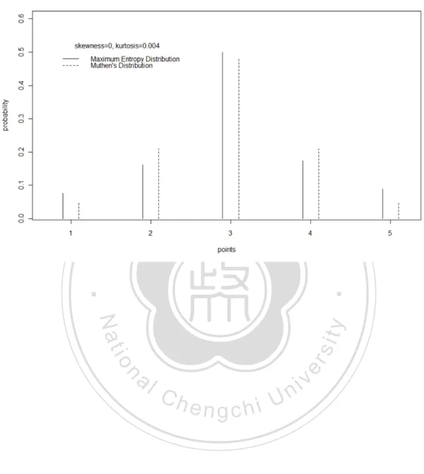
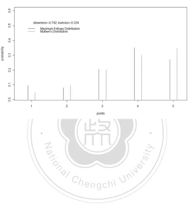
(30) uniform distribution, beta distribution, exponential distribution, gamma distribution, Possion distribution, and normal distribution. All of these are members of the maximum entropy family subjecting to different constraints (Theil & Fiebig, 1984). This phenomenon implies that the maximum entropy principle might be a general principle for probability distributions. In order to illustrate the characteristics of the maximum entropy distribution, the. 政治大. 5 category discrete probability distributions in Muthén’s research (Muthén & Kaplan,. 立. 1985) and the discrete maximum entropy distributions with the same skewness and. ‧ 國. 學. kurtosis are presented in Figure 1 to Figure 5. In addition, the maximum entropy. ‧. probability distribution of the skewness 0 and kurtosis 2.898 is presented in Figure 6.. Nat. io. sit. y. It can be seen through these figures that the maximum entropy distributions are. er. smoother than the Mutén’s distributions.. al. n. v i n C hit can be seen thatUthe discrete maximum entropy Through the discussion above, engchi. distributions are typical, smooth, and have no empty category. All these properties make them a proper choice from infinite probability distributions satisfying the specified constraints. Therefore, the MEP which chooses the discrete maximum entropy probability distributions with specified constraints is also a reasonable and attractive procedure to generate data with specified parameters for Monte Carlo method of the robustness researches.. 19.

(31) Section 3 the Solution of the Maximum Entropy Procedure Since the MEP is a reasonable and suitable procedure for choosing the discrete probability distributions with specified constraints for psychological data, the way to obtain the maximum entropy distribution is the next problem when the MEP is implemented. Traditionally the Lagrange multiplier is used to solve this problem (Jaynes, 1957b; Kapur & Kesavan, 1992; Kesavan & Kapur, 1989). The Lagrange. 政治大. multiplier provides a strategy for finding the maximum or minimum of a function. 立. subject to constraints and thus is suitable for this problem. The Lagrange function  to. ‧ 國. 學. maximize the information entropy of discrete probability distribution subjects to. ‧. specified constraints is defined as, k. y. Nat. ( p1 ,..., pk , 0 , 1 ,...m )  H ( p1 ... pk )  0 ( pi  1)  1C1 ( p1 ,..., pk )...  m C m ( p1 ,..., pk ). er. io. sit. i 1. al. n. v i n are the Lagrange C multipliers, C ,..., C are the constraints h e n gandc the hi U. where 0 ,...m. 1. (10).. m. specified by the researchers for p1 ,..., pk . In addition to the constraints C1 ,..., C m , there k. is a constraint  pi  1 , and thus the total number of constraints is m+1. By solving i 1. the partial differentiations of each variables of the Lagrange function  equal to 0 as follows,.  p1 ,..., pk ,0 ,1 ,...,m  ( p1 ,..., pk , 0 , 1 ,..., m )  0. (11).. the solutions of p1 to pk which satisfying the m+1 constraints can be attained. After the. 20.

(32) probabilities p1 to pk are attained, the data from the discrete maximum entropy probability distribution with the specified parameters can be generated through sampling via inversion of the cumulative mass function (cmf) discussed in previous chapter.. Section 4 the Maximum Entropy Procedures Proposed in this Research. 政治大. Through the discussion of previous sections, it can be seen that the properties of. 立. the discrete maximum entropy distributions makes the MEP a reasonable and suitable. ‧ 國. 學. discrete probability distribution choosing procedure for simulating data with specified. ‧. parameters for Monte Carlo researches. The solutions of the maximum entropy. Nat. io. sit. y. distributions are also presented make the implementation of the MEP realistic.. er. Therefore, the MEP would be proposed to choose the discrete probability distribution. al. n. v i n C hsets of parameters chosen with the specified parameters. The e n g c h i U for the implementation of MEP in this research are the set of 4 parameters, mean, variance, skewness and kurtosis and the set of 2 parameters, skewness and kurtosis. The set of the 4 parameters are chosen for the MEP proposed in this research. because most real-world distributions are characterized by mean, variance, skewness and kurtosis as noted by Fleishman (1978). In addition, the mean and variance of the discrete data could not be simply transformed as these parameters of the continuous. 21.

(33) data. With different mean and variance, the shapes of discrete probability distributions are different even with same skewness and kurtosis. With the 4 parameters specified, the discrete probability distributions specified are less uncertain since there is more information. Therefore, the Maximum Entropy Procedure with 4 parameters (MEP-4) is proposed with the 4 parameters are specified in this research for Monte Carlo researches with all the information is known.. 政治大. The set of the 2 parameters are chosen for the MEP proposed in this research. 立. because the degree of non-normality is most often evaluated only by the skewness and. ‧ 國. 學. kurtosis values (Muthén & Kaplan, 1985). Because the mean and variance values of. ‧. normal distributions can be set arbitrarily, most researchers also only manipulated. Nat. io. sit. y. these values in their robustness studies (e.g., Curran et al., 1996; Hampel, 1973; Lei &. er. Lomax, 2005). Therefore, to generate variables for robustness research of. al. n. v i n C h Procedure withUthese 2 parameters specified non-normality, the Maximum Entropy engchi (MEP-2) is proposed. In this research, the MEP is proposed for generating the discrete data with the specified parameters for robustness researches. The sets of the specified parameters are the set of mean, variance, skewness and kurtosis and the set of skewness and kurtosis. The details of these procedures and the statistical program used to implement these procedures are presented, evaluated and discussed in next chapters.. 22.

(34) Chapter 3 the Maximum Entropy Procedure with the 4 Parameters (MEP-4) One of the aims of this research is to propose the maximum entropy procedure with 4 parameters which estimate the discrete maximum entropy distribution when mean, variance, skewness and kurtosis are specified. The R package for the MEP-4 is also provided for researchers to implement the MEP-4 to obtain the discrete. 政治大. maximum entropy distribution with specified parameters and to sample the data from. 立. this distribution under a specified number of categories automatically. For. ‧ 國. 學. implementing the MEP-4, the solutions of the MEP-4 and the details of the. ‧. corresponding R package are discussed and presented in this chapter.. io. sit. y. Nat. er. Section 1 the Solution of the MEP-4. al. n. v i n C h maximum entropy The MEP-4 estimates the discrete e n g c h i U distribution when mean,. variance, skewness and kurtosis are specified. The parameters for a discrete variable x with k categories are defined as follows: k.   E  X    p i xi  M 1 .. (12a). i 1. 2.  k    E ( X )  E ( X )   x pi    xi pi   M 2  M 1 2 . i 1  i 1  2. 2. 2. k. 2 i. 23. (12b).

(35) 3. 3 k k  k 3  k   3 3 2  1  E X  E ( X ) /    xi pi  3 xi pi  xi pi  2  xi pi   i 1 i 1 i 1  i 1    M  3M 2 M 1  2M 13  3 3 2 2 (M 2  M 1 ). 2 2 k  k 2   x p   x p    i i  i i   i 1  i 1 . (12c)  2  E X  E ( X )4 /  4 2 4 k k k  k 4  k   k   3 2    xi pi  4 xi pi  xi pi  6 xi pi   xi pi   3  xi pi   i 1 i 1 i 1 i 1  i 1   i 1    M  4M 3 M 1  6M 2 M 12  3M 14  4 ( M 2  M 12 ) 2. 2 k  k 2   x p   x p     i i i i  i 1  i 1   . 政治大. 立. (12d). where  ,  , 1 and  2 are the mean, variance, skewness and kurtosis respectively and 2. ‧ 國. 學. M1 to M4 are the values of the first 4 moments from 0 of variable x. It can be seen that. ‧. the values of the 4 parameters and the first 4 moments from 0 could be transformed. sit. y. Nat. io. n. al. er. into each other. The first 4 moments could be computed from the 4 parameters through the following formulas, M1  . Ch. engchi. i n U. v. (13a). M2   2  2. (13b). M 3  1 3  3 2   3. (13c). M 4   2 4  4 1  3  6 2 2   4. (13d). Therefore, while the 4 parameters are specified, the first 4 moments are also specified. The constraints of the 4 parameters could be expressed as constraints of the. 24. 2.

(36) 4 moments. Since the formulas of the first 4 moments are simpler, the constraints while maximizing entropy in the MEP-4 are k. p i 1. i. 1. k. p x i 1.  M1. (14b). 2 i.  M2. (14c). 3 i i.  M3. (14d). i i. k. p x i 1 k. i. p x i 1 k. p x i 1. (14a). i. 4 i. 政治大.  M4. 立. (14e). The solution of maximum entropy distribution with the first 4 moments specified are. ‧ 國. 學. discussed by Jaynes (1957a) and the problem can be expressed as the Lagrange. ‧. function as. k. k. y. i 1. k. i 1. i 1. sit. i 1. k. k. io.  2 ( pi x 2  M 2 )  3 ( pi x 3  M 3 )  4 ( pi x 4  M 4 ). n. al. Ch. engchi U. er. Nat. ( p1 ,..., pk , 0 , 1 , 2 , 3 , 4 )  H ( p1 ... pk )  0 ( pi  1)  1 ( pi x  M 1 ). v ni. i 1. (15). and the solution is. . pi  exp  0  1 xi  2 xi2  3 xi3  4 xi4. . (16).. Although there’s a solution for the MEP-4, the closed-form solution of pi does not exist with unknown values of 0 , 1 , 2 , 3 , 4 . The numerical optimization techniques are used to estimate the values of 0 , 1 , 2 , 3 , 4 thus allowing a direct calculation of pi. The most frequent approach for the solution of optimizing the. 25.

(37) maximum entropy adopts the iterative Newton’s method for continuous variables and was proposed (Mohammad-Djafari & d'Electricite, 1992; Zellner & Highfield, 1988). The iterative Newton’s method for continuous variables is modified for discrete variables in the MEP-4. The iterative Newtown’s method in the MEP-4 is illustrated as follows. The formula (16) could be seen as a function of 0 , 1 , 2 , 3 , 4 , and thus the formulas (14a) to (14e) would become. 立. i. k. i 1. i 1. exp  0  1 xi  2 xi2  3 xi3  4 xi4  M 2. 3 i. exp  0  1 xi  2 xi2  3 xi3  4 xi4  M 3. 4 i. exp  0  1 xi  2 xi2  3 xi3  4 xi4  M 4. . . . io. k. x. . 2 i. Nat. k. x. . .  1 xi  2 xi2  3 xi3  4 xi4  M 1. . al. (17c) (17d). n. v i n C h function G is defined For expressing conveniently, another e n g c h i U as below, G ( )   x exp    x   x   x   x  i 1. k. r. i 1. r i. 0. 1 i. 2 2 i. 3 3 i. 4 4 i. (17b). ‧. x. 0. y. k. (17a). 學.  x exp  i 1. .  1 xi  2 xi2  3 xi3  4 xi4  1. sit. i 1. 0. er. k. ‧ 國.  exp . 政治大. (17e). (18). Where λ is a vector that   0 , 1 , 2 , 3 , 4 and r is from 0 to 4. With initial values of  set as 0  00 , 10 , 02 , 03 , 04 , the equations of (17a) to (17e) could be expanded in the Taylor’s series and expressed as M r  G r ( ).  G r (0 )  (0  00 ) g r 0  (1  10 ) g r1  (2  02 ) g r 2  (3  03 ) g r 3  (4  04 ) g r 4 (19). 26.

(38) where g rq is Gr q evaluated as 0 and k. . g rq   xir  q exp  0  1 xi  2 xi2  3 xi3  4 xi4. . (20). i 1. and q is from 0 to 4. Therefore the formulas (17a) to (17e) could be restated as follows:  g 00 g 01 g 02 g g g  10 11 12  g 20 g 21 g 22   g 30 g 31 g 32 g g g  40 41 42. 0 0 g 03 g 04   0  1  G0 ( )    0  0 g13 g14   1   M 1  G1 ( )  g 23 g 24   20    M 2  G2 (0 )  g 33 g 34   30   M 3  G3 (0 )      g 43 g 44   40   M 4  G4 (0 )    . 0. 立. 政治大. is the vector of  00 ,  10 ,  20 ,  30 ,  40 . The formula (21) is solved. 學. ‧ 國. where  r0  r  0r . . (21). when 1  0   0 , else 1 becomes our new vector of trial lambdas, and iterations. ‧. continue until  0 becomes appropriately small. When the iteration stops, the. sit. n. al. er. io. solution of the MEP-4.. y. Nat. estimated  vector is used to estimate the maximum entropy distribution and also the. Ch. engchi. i n U. v. Section 2 the Details of the R Package for the MEP-4 The R package for the MEP-4 which implements the MEP-4 could estimate the discrete maximum entropy distribution with the 4 specified parameters and sample the specified number of samples with specified sample size from this distribution is also provided in this research. The samples are generated through sampling via inversion of the cumulative mass function (cmf) discussed in Chapter 1. The details of the. 27.

(39) package would be introduced as follows. 1. Information Encoded: The specified information need to be encoded is, number of categories, specified values of mean, variance skewness and kurtosis. The number of samples needed and the corresponding sample size are optional information, but the sampling process starts only when these values are encoded. 2. Estimation:. 立. 政治大. The Newtown iterative method in previous section is applied to estimate the. ‧ 國. 學. Lagrange Multipliers as well as the maximum entropy distribution. While. ‧. estimating, the parameters encoded would be transformed into the first 4. Nat. io. sit. y. moments. The range of values of encoding categories is transformed into -1. er. to 1 in order to reduce the effect of the fourth exponentiation which would. al. n. v i n C hvalues when the absolute give great weight to bigger e n g c h i U values larger than 1 and thus affect the estimation process in the MEP-4.. 3. Starting Values: The initial starting values of λ would generate a discrete uniform distribution. The value of 00 is the only value not 0 in vector λ. The set of starting values is the same as the program presented by Mohammad-Djafari and d’Electricite (1992).. 28.

(40) 4. Stop Criteria: There are 3 stop criteria of the iteration process. The iteration would be seen as having converged and thus stop when the sum of the difference of lambdas is smaller than 10-20. The iteration also stops while the inverse matrix of g rq is unable to calculate; which implies that either the iteration has converged or the parameters were poorly specified. The iteration also stops when the. 政治大. number of iterations exceeds the pre-set maximum number of iterations. 立. (1,000 is the default value).. ‧ 國. 學. 5. Output:. ‧. The output includes the estimated maximum entropy distribution and the. Nat. io. sit. y. corresponding descriptive statistics, such as the specified 4 parameters and. er. the obtained 4 parameters of the estimated probability distribution, if the. al. n. v i n solution is successfullyC generated. the error message presents h e n gOtherwise, chi U when the iteration fails. The generated data is also listed if the number of samples and sample size are encoded. The output would also be saved automatically.. 29.

(41) Chapter 4 Evaluation of the Maximum Entropy Procedure with 4 Parameters The MEP-4 is proposed with the corresponding R package which implements the MEP-4 is provided in this research. The MEP-4 is evaluated through evaluating the quality of the solutions obtained through the R package. 2 simulated studies were conducted to confirm the possible generated parameter spaces for accurate solutions. 政治大. of the MEP-4. In the study 1, the number of categories of discrete measures and the. 立. values of the 4 parameters were manipulated to evaluate the solutions of the MEP-4 in. ‧ 國. 學. these conditions for possible generated parameter spaces. In the study 2, the 4. ‧. parameters combinations from the real existed probability distributions were encoded. Nat. io. sit. y. into the R package for the MEP-4 to understand the accuracy and confirm the possible. n. al. er. generated parameter spaces of the MEP-4. The designs and results of these 2 studies are presented in this chapter.. Ch. engchi. i n U. v. Section 1 Research Design of the Study 1 In order to evaluate the quality of solutions of the MEP-4 obtained through the corresponding R package, a simulation study was conducted. Theoretically, the values of 4 parameters and the nature of discrete probability distributions would restrict each other. However, the relations are not clear. For the sake of prudence, the combinations. 30.

(42) of these parameters in particular ranges and 2 different numbers of categories were manipulated, although some combinations may be improper as known, such as combinations with relatively large mean and skewness or with relatively large variance and kurtosis. The details of the 5 variables manipulated in the simulation study were as follows: 1. Number of categories of discrete measures.. 政治大. Two levels were in this variable, consisting of 6 and 7 categories. The. 立. applied number of categories is restricted by the number of constraints.. ‧ 國. 學. The number of constraints in the MEP-4 is 4+1=5 and the proper. Nat. er. io. 2. Mean.. sit. categories manipulated in this study was 6 and 7.. y. ‧. applied number of categories is larger than 5; therefore, the number of. al. n. v i n C hwere 19 and 23 levels For this variable, there e n g c h i U in this variable in 6 and 7 categories respectively. The levels of the mean values ranged from 1.25 to 5.75 in 6 categories and 1.25 to 6.75 in 7 categories and the interval was set as 0.25. The extreme mean values 1, 6, and 7 were not included because the corresponding variance values could only be 0. Therefore, the levels were from 1.25 to 5.75 for 6 categories, and from 1.25 to 6.75 for 7 categories.. 31.

(43) 3. Variance: There were 8 levels in this variable. The levels of variance values were arbitrarily set from 0.25 to 2 and the interval was also set as 0.25. 4. Skewness: There were 25 levels in this variable. The levels of skewness values were arbitrarily set from -3 to 3 and the interval was also set as 0.25. 5. Kurtosis:. 立. 政治大. There were 33 levels in this variable. According to the rule from. ‧ 國. 學. Pearson’s inequality (1916): Skewness 2  Kurtosis  2 , the minimal. ‧. possible kurtosis value would be restricted by the skewness value of the. Nat. io. sit. y. same probability distribution. Therefore, the levels of the kurtosis value. n. al. er. were set from the minimal possible value to this value plus 9. The. Ch. interval was also set as 0.25.. engchi. i n U. v. The last 4 variables contributed to 140,600 combinations in 6 categories discrete measures and 170,200 combinations in 7 categories discrete measures. The solutions were evaluated through the differences between the previously specified 4 parameters and the corresponding 4 parameters of the estimated discrete maximum entropy distributions. The solutions would be seen as successfully generated when the 4 absolute differences between the specified and the estimated parameters were all. 32.

(44) smaller than 0.001.. Section 2 Results of the Study 1 Since the accuracy was the criteria of successfully generation, the generated rate was only used to evaluate the possible generated parameter spaces of the MEP-4 and was defined as the ratio of the solutions generated successfully to all the combinations. 政治大. of the manipulated variables. The overall generated rate was 13.48%. The generated. 立. rate was 8.24% for 6 categories and 17.80% for 7 categories. The descriptive statistics. ‧ 國. 學. and the root mean squared differences (RMSDs) of differences between the. ‧. previously specified and the 4 parameters from the estimated discrete maximum. Nat. io. sit. y. entropy distribution of the MEP-4 under 6 and 7 categories are presented in Table 1.. er. Some trends could be seen of the 4 parameters of the generated combinations.. al. n. v i n C h was presented The correlation matrix of the 4 parameters e n g c h i U in Table2. It can be seen that the correlations between mean and skewness and variance and kurtosis were both negative as expected. However, the relations between these parameters are not linear, and the Pearson correlation is not the best tool to describe the relations in this situation. Therefore, the plots of each combination of 2 parameters of these 4 parameters were also presented in Figure 7 to 12. These plots could be referred for researchers who use the MEP-4 to estimate the maximum entropy distributions.. 33.

(45) Section 3 Research Design of the Study 2 The overall generated rate of the MEP-4 in study 1 was only 13.48% under the conditions manipulated. The impermissible combinations of the 4 specified parameters might be the reason for the low generated rate, but the other possibility of inaccuracy solutions also existed. Therefore, a simulated study whose aim was to evaluate the solutions of the MEP-4 with existed combinations of the 4 parameters of. 政治大. discrete probability distributions was conducted to verify the cause. If the generated. 立. rate of this study is high, it implies that the low generated rate in study 1 is caused by. ‧ 國. 學. the improper combinations of the 4 parameters but not the low accuracy. If the. ‧. generated rate is still low, it implies the reason is the inaccurate solutions.. Nat. io. sit. y. The discrete probability distributions of 6 and 7 categories were also researched. er. in this study as in the study 1. The value of probability of each category was. al. n. v i n C hcombinations of theU4 parameters. The probability manipulated to generate the existed engchi of each category ranges from 0 to 0.95 and the interval is 0.05 to form existed probability distributions. The rule of manipulation could be explained through following example. According to the rule, when the probability of category 1 is 0.95, there were 5 different discrete probability distributions existed. They were probability distributions with category 2, 3, 4, 5 and 6 were probability 0.05 separately and with other categories were probability 0. When the probability of category 1 is 0.9, there. 34.

(46) were 15 different discrete probability distributions existed. 5 of them were probability distributions with category 2, 3, 4, 5 and 6 were probability 0.10 separately and with other categories were probability 0. Others were probability distributions with 2 of category 2, 3, 4, 5 and 6 were probability 0.05 and with other categories were probability 0. Through this rule, many existed different probability distributions could be generated. After the probability distributions were generated, the corresponding 4. 政治大. parameters were calculated. The generated discrete probability distributions are. 立. 53,124 and 230,223 of 6 and 7 categories relatively according to the manipulation rule.. ‧ 國. 學. The corresponding 4 parameters of these probability distributions were all encoded. Nat. n. al. er. io. sit. The criterion of successfully generation is the same as study 1.. y. ‧. into the R package for the MEP-4 to obtain and evaluate the solution of the MEP-4.. C h2 Section 4 Results of the Study e. ngchi. i n U. v. The generated rates of these combinations of 6 and 7 categories discrete probability distributions are both as high as 100%. The descriptive statistics and the root mean squared differences (RMSDs) of differences between the 4 previously specified parameters and the corresponding 4 parameters of the estimated maximum entropy distributions under 6 and 7 categories are presented in Table 3. The high generated rate indicates that the solutions of the MEP-4 obtained through the. 35.

(47) corresponding R package are estimated quite accurate. Therefore, the low generated rate is caused by the impossible existed combinations of the 4 parameters. The correlation matrix of the 4 parameters in this study is presented in Table 4. The correlation matrixes are similar between the successfully generated 4 parameters in study 1 and the existed parameters in study 2. It shows that relation between the possible generated combinations of the 4 parameters in study 1 and the. 政治大. existed 4 parameters may be similar. It also enhances our confidence that the low. 立. generated rate is caused by the improper generated combinations of the 4 parameters.. ‧ 國. 學. The plots of the combinations of each the 2 parameters are presented in Figure 13 to. ‧. Figure 18. It could be also referred for researchers who use the MEP-4 to estimate the. Nat. io. sit. y. maximum entropy distributions.. er. The results of the study 2 show that the existed combinations of the 4 parameters. al. n. v i n C hand the relationships can be 100% successfully generated e n g c h i U of the generated 4. parameters and the existed parameters are similar. All these results support that the low generated rate is caused by the improper combinations of the 4 specified parameters. It can be seen that the MEP-4 can estimate probability distributions with specified parameters precisely.. 36.

(48) Chapter 5 the Maximum Entropy Procedure with 2 Parameters (MEP-2) The maximum entropy procedure with 2 parameters estimates the discrete maximum entropy distribution for specified the values of skewness and kurtosis is proposed in this chapter. The R package for the MEP-2 to implement the MEP-2 is also provided for researchers to estimate the discrete maximum entropy distribution. 政治大. with the specified values of skewness and kurtosis under a specified number of. 立. categories and the samples the samples from this probability distribution. Since there. ‧ 國. 學. are only 3 constraints in the MEP-2, the applied number of categories of the MEP-2 is. ‧. much smaller than the MEP-4. Therefore, for the robustness studies for the impact of. Nat. io. sit. y. non-normality, the MEP-2 might be more practical. For implementing the MEP-2, the. n. al. er. solutions and the details of the corresponding R package are discussed and presented in this chapter.. Ch. engchi. i n U. v. Section 1 the Solution of the MEP-2 As in the MEP-4, the solution of the MEP-2 theoretically can be attained through Lagrange Multiplier. The two constraints in MEP-2 should be formulas (12c) and (12d) and the corresponding Lagrange function Λ is. 37.

(49) k. ( p1 ,..., pk , 0 , 1 , 2 )  H ( p1 ... pk )  0 ( pi  1)  1 (. M 3  3M 2 M 1  2M 13 3 2 2 1. i 1.  2 (.  1 ). (M 2  M ). M 4  4M 3 M 1  6M 2 M 12  3M 14  2 ) ( M 2  M 12 ) 2. (22). where M1 to M4 are the values of the first 4 moments from 0 of the estimated k categories discrete probability distribution. However, the explicit solution of probability of each category p1 ,..., pk is hard to. 治政 obtain with such complicated constraints, thus the iterative 大 Newton’s method in the 立 ‧ 國. 學. MEP-4 could not be adopted (Kapur & Kesavan, 1992). After many different methods were tried, the numerical technique Simplex (Nelder & Mead, 1965) is chosen to. ‧. solve this problem. The function minimized through Simplex is as follows,. y. Nat. (M 2  M ). n. al. Ch. sit. 3 2 2 1. M 4  4 M 3 M 1  6 M 2 M 12  3M 14  1 ) |  | (  2 ) | ( M 2  M 12 ) 2. er. io.  H ( p1 ... pk ) | (. M 3  3M 2 M 1  2 M 13. engchi. i n U. v. (23). where M1 to M4 are the values of the first 4 moments from 0 of the estimated k categories discrete probability distribution, 1 and  2 are the specified skewness and kurtosis. Since the above function achieves its minimum as the differences of the previous specified and obtained parameters are 0 and the entropy is at its maximum, the solution obtained through minimizing this function would be the one with the maximum entropy and with the specified constraints fulfilled.. 38.

(50) Section 2 the Details of the R Package for the MEP-2 The R package for the MEP-2 to implement the MEP-2 could estimate the discrete maximum entropy distribution with the specified 2 parameters is provided in this research. The package also could sample the specified number of samples with specified sample size from the estimated probability distribution. The samples are also generated through sampling via inversion of the cumulative mass function (cmf). 政治大. discussed in Chapter 1. The details of the R package would be introduced to facilitate. 立. 學. ‧ 國. the usage of the package.. 1. Information Encoded:. ‧. The information need to be encoded is: number of categories, values of. Nat. io. sit. y. skewness and kurtosis. The number of samples need and the sample size are. n. al. er. optional information, but the sampling process starts only when these. Ch. information are encoded.. engchi. i n U. v. 2. Estimation: The probability of each category is estimated directly through minimizing value of formula (23). The minimize process is conducted through the numerical optimization technique Simplex (Nelder & Mead, 1965) in R. The number of dimensions to be optimized is k-1 to implement the constraint. 39.

(51) k. p i 1. i.  1 . The range of values of encoding categories is transformed into -1. to 1 as was the case in the MEP-4 to reduce the effect of the fourth exponentiation. 3. Starting Value: The initial set of starting values is assigned to be the discrete uniform distribution which is the probability distribution with the largest information. 政治大. entropy without any constraints. If there’s no accepted solution, i.e, any one. 立. of the difference of parameters is larger than 0.001, the set of estimated. ‧ 國. 學. probability is modified as a new set of starting values. Moreover, in order to. ‧. finding the global maxima, multiple sets of starting values are used. The. Nat. io. sit. y. default number of the starting values sets is 10 and the number could be. n. al. er. modified by the users. 4. Stop Criteria:. Ch. engchi. i n U. v. There are 2 stop criteria in the MEP-2. While the difference of the value of formula (23) is smaller than 10-20, the iteration would be seen as converged and thus stop. The iteration would also stops when the number of iterations exceeds the maximum number of 500. 5. Output: The output of the MEP-2 includes the maximum entropy distribution and the. 40.

(52) corresponding specified and estimated 2 parameters if the solution is successfully generated. Otherwise, the error message presents. The generated data is also listed if the number of samples and sample size are encoded. The output would be saved automatically.. 立. 政治大. ‧. ‧ 國. 學. n. er. io. sit. y. Nat. al. Ch. engchi. 41. i n U. v.

(53) Chapter 6 Evaluation of the Maximum Entropy Procedure with 2 Parameters The MEP-2 is proposed with the corresponding R package which implements the MEP-2 in this research. The MEP-2 is evaluated through evaluating the quality of the solutions obtained through the R package. A simulation study is conducted to evaluate the accuracy and parameter space of the MEP-2, in which the number of categories of. 政治大. discrete measures and the values of the 2 parameters are manipulated. The design and. 立. results of the study are presented in this chapter.. ‧. ‧ 國. 學. Section 1 Research Design of the Study 3. Nat. io. sit. y. In order to evaluate the quality of the solutions obtained through the R package. er. for the MEP-2, a simulation study with a similar design of study 1 was conducted.. al. n. v i n C h in this study were Since the only manipulated parameters e n g c h i U skewness and kurtosis and the possible combinations of the values of skewness and kurtosis were proposed by Pearson (1916), the manipulated combinations of the 2 parameters would all be possible. Therefore, the parameters combinations should be all possible to generate. The details of the variables manipulated are as follows: 1. Number of categories of discrete measures. There were 2 levels in this variable, 4 and 5 categories. As in the MEP-4,. 42.

(54) the applied number of categories of the MEP-2 is restricted by the number of constraints. The number of constraints in the MEP-2 is 2+1=3 and the proper applied number of categories is larger than 3; therefore, the numbers of categories manipulated in this study were 4 and 5. 2. Skewness.. 政治大. There were 25 levels in this variable. The levels of skewness values. 立. were arbitrarily set from -3 to 3, and the interval was set as .25.. ‧ 國. 學. 3. Kurtosis.. ‧. There were 33 levels in this variable. The levels of kurtosis values were. Nat. io. sit. y. set from the minimal possible value according to the corresponding. er. skewness to this value plus 9, and the interval was set as .25.. al. n. v i n C hwere estimated in both 925 parameters combinations e n g c h i U 4 and 5categories discrete measures. The solutions are evaluated through the differences between the previously specified 2 parameters and the corresponding 2 parameters of the estimated probability distributions. The solution would be seen as successfully generated when the absolute values of the 2 differences between the specified and the estimated parameters were both smaller than 0.001.. 43.

(55) Section 2 Results of the Study 3 The generated rate was defined as the ratio of the solutions generated to all the combinations of specified parameters as study 1. The generated rate of the MEP-2 in both 4 and 5 categories were 100%. The MEP-2 can successfully generate solutions of all parameter space of skewness and kurtosis through the boundary of Pearson (1916) as expected. The descriptive statistics and RMSDs (root mean squared differences). 政治大. were presented in Table 5. It can be seen that with the 2 parameters specified, the. 立. MEP-2 can precisely estimate the discrete probability distributions with specified. ‧ 國. 學. parameters through the corresponding R package.. ‧. n. er. io. sit. y. Nat. al. Ch. engchi. 44. i n U. v.