國
立
交
通
大
學
生醫工程研究所
碩
士
論
文
使用 T1 權重和擴散張量磁振造影影像之腦
部影像模板建構
Construction of Brain Templates using T1-weighted and
DT MRI Data
研 究 生:沈于涵
指導教授:陳永昇 教授
使用 T1 權重和擴散張量磁振造影影像之腦部影像模板建構
Construction of Brain Template using T1-weighted and DT MRI Data
研 究 生:沈于涵 Student:Yu-Han Shen
指導教授:陳永昇 Advisor:Yong-Sheng Chen
國 立 交 通 大 學
生 醫 工 程 研 究 所
碩 士 論 文
A ThesisSubmitted to Institute of Biomedical Engineering College of Computer Science
National Chiao Tung University in partial Fulfillment of the Requirements
for the Degree of Master
in
Computer Science
December 2012
Hsinchu, Taiwan, Republic of China
Brain template construction using T1-weighted
and DT MRI data
A thesis presented
by
Yu-Han Shen
to
Institute of Biomedical Engineering
College of Computer Science
in partial fulfillment of the requirements for the degree of
Master
in the subject of
Computer Science
National Chiao Tung University Hsinchu, Taiwan
Brain template construction using T1-weighted and DT MRI data
Copyright © 2012 by
i
摘 要
本研究之主要目標在使用 T1 權重和擴散張量磁振造影影像來建立腦部影像模板。 近年來的研究中,許多腦部影像模板是建構在一個名為 ICBM-152 的模板空間,例如: ICBM452、ICBM DTI-81 和 IIT DT 腦影像模板。然而,除了個人化變異之外,腦部結 構會受種族、性別、年齡或疾病的影響而有所差異。因此,我們發展了一套系統流程, 可針對所研究的族群建構其腦影像模板。為了減少在建構模板過程中所造成的影像失真, 我們使用了對稱且微分同構的對位演算法,以同時提供正、逆形變場。另外,我們也提 出可結合 T1 權重和擴散張量磁振造影影像資訊的目標函式,來改善影像對位的精準 度。 擴散張量影像是由對雜訊敏感的擴散權重影像所估計而成。在本研究中,我們嚴謹 地考量在擴散張量磁振造影影像的所有處理細節。首先,我們使用了 Medical Image Navigation and Research Tool by INRIA (MedINRIA)的方法來估計張量,此工具可適用於 低雜訊比的擴散權重影像,並可確保所有估計出的張量皆為正定矩陣。為了更進一步保 存所估計出張量的良好特性,我們使用了對數-歐幾里德的架構,以避免出現張量膨脹 效應與非正特徵值的問題。 在此研究中,我們針對六十四個受測者的影像來建構腦影像模板。首先,我們使用 剛性對位演算法將磁振造影對位到擴散權重之基準影像,以確保此二種影像對位在同一 個座標空間。接著,我們在所有的影像中,找出一個對位到其他受測者影像時,擁有最 小形變量的受測者作為代表。接著,我們重複地進行影像對位及逆形變場平均,直到影 像模板空間收斂到一個穩定的狀態。最後,即可在此空間建構代表性受測者影像模板和 平均影像模板。 本研究使用了兩種系統評估方法,其一是利用特徵值和特徵向量的組合,來評估兩 個不同張量之間的重疊程度。另一個方法,則是利用擴散張量磁振造影來評估磁振造影 的對位精準度。評估的結果顯示,若在非剛性對位演算法之中,同時使用 T1 權重和擴 散張量磁振造影資訊,則非剛性對位的精準度可以得到改善。並且,結果也顯示我們所
ii
建立出的影像模板與對位到此模板空間的受測者影像有很高的相關性。因此,我們所提 出的腦部影像模板建構流程與相關對位演算法,可以為所研究的族群提供一個腦結構分 析的座標空間。
iii
Abstract
This study aims at the development of a construction algorithm for brain templates using T1-weighted and diffusion tensor (DT) magnetic resonance imaging (MRI) data. Recently, several brain templates developed in the ICBM-152 stereotactic space, such as ICBM452, ICBM DTI-81 atlas, and IIT DT brain template. In addition to inter-subject variation, however, the brain structures vary with races, genders, ages, and diseases. Hence, a construction algorithm of the stereotactic space for a specific study group can facilitate the structure analysis of the brains. Moreover, we improved the accuracy of registration procedure to reduce the image distortion during the template construction procedure. First, a symmetric and diffeomorphic non-rigid registration algorithm was used to provide both forward and inverse deformation fields. Also, we proposed an objective function which simultaneously utilized both T1-weighted and DT data to improve the accuracy of registration.
The DT image is estimated from noise-sensitive diffusion-weighted images (DWIs). All details of DT-MRI processing procedure were carefully considered in this study. First, DT images were estimated from DWIs by the MedINRIA tensor estimation tool, which can tolerate the low signal-to-noise ratio (SNR) in clinical MRI and ensure the positive definiteness of all tensors. For preserving the good property of estimated tensors, Log-Euclidean metrics was used to avoid the problems of the tensor swelling effect and non-positive eigenvalues.
In this study, 64 normal subjects were recruited for MRI scanning and template construction. First, we rigidly registered the MRI image to baseline DWI image for each subject to align both modalities of images in the same stereotactic space. Second, a representative subject was chosen as the one having the smallest deformation magnitude when registering to other subject images. Third, each subject image was registered to the temporary template, which was initialized as the image of the representative subject. The average of the obtained inverse deformation fields was applied to the image of the representative subject to update the temporary template. Iteratively applying the third step until the template image converges. Finally, we constructed a representative template and an average template in this converged space.
In this study, two criteria were used to evaluate the constructed template images and the registration accuracy, including the DTI differences and overlaps between each subject and
iv
the template. The evaluation results showed that the accuracy of non-rigid registration was improved by simultaneously utilizing both T1-weighted and DT data. Furthermore, the results displayed a high correlation between the proposed template and registered subject images. Consequently, the proposed brain template construction could provide a stereotactic space for a specific subject group.
v 致 謝 非常感謝我的指導教授陳永昇老師和陳麗芬老師,對我這兩年來在研究上以及為人處事 上的指導、教誨、照顧與幫助,真的讓我學習到很多,也得到很大的成長。感謝鍾孝文 老師、陳麗芬老師和王才沛老師在口試中所提出的各方面建議與指導,也很感謝老師們 對我論文的審視與指正,都讓我獲益匪淺。很高興這兩年能夠待在歡樂的 BSP 實驗室, 感謝實驗室的所有夥伴們,與我一同打拼、一同學習成長、一起玩樂,也很感謝大家所 有的關照與幫助。最後也感謝我的家人與朋友們的陪伴、感謝社團夥伴們的鼓勵與支持, 非常感謝大家。
Contents
List of Figures ix List of Tables xi 1 Introduction 1 1.1 Backgrounds . . . 2 1.2 Motivation . . . 32 Material and Methods 7 2.1 Materials . . . 8 2.2 Methods . . . 8 2.2.1 Template construction . . . 8 2.2.2 Preprocessing procedure . . . 13 2.2.3 Feature extraction . . . 15 2.2.4 Image registration . . . 16 2.2.5 DTI reorientation . . . 19 2.2.6 Log-Euclidean metrics . . . 20 2.2.7 Evaluation methods . . . 21
3 Results and Discussion 23 3.1 Feature comparison . . . 24
3.2 Curve analysis . . . 28
3.3 Framework comparision . . . 30
3.4 Average template and representative template . . . 30
3.5 Comparison with different DTI template construction . . . 37
4 Conclusions 39 4.1 Conclusions . . . 40
4.2 Future works . . . 40
Bibliography 43
List of Figures
1.1 DTI introduction . . . 3 1.2 ICBM 152 templates . . . 4 1.3 Different templates . . . 5 2.1 Intra-subject alignment . . . 9 2.2 Brief flowchart . . . 10 2.3 Detailed flowchart . . . 11 2.4 Tensor reorientation . . . 13 2.5 MRI preprocessing . . . 14 2.6 DTI preprocessing . . . 14 2.7 Feature extraction . . . 15 2.8 Intensity contrast . . . 17 2.9 Correlation ratio . . . 183.1 Mean OVL with different features (a) The OVL between registered subjects and representative template (b) The OVL between registered subjects and average template . . . 28
3.2 (a) Mean DTI error (b) Mean MRI error . . . 29
3.3 Number of voxels with average template in different FA value bins . . . 31
3.4 Representative template . . . 33
3.5 Average template . . . 34
3.6 Registering templates to ICBM452 atlas . . . 35
3.7 Outliers . . . 38
List of Tables
3.1 Mean OVL with average template in whole brain . . . 24
3.2 Mean OVL with average template in white matter . . . 24
3.3 Mean OVL with representative template in whole brain . . . 25
3.4 Mean OVL with representative template in white matter . . . 25
3.5 Mean ErrorDT I in whole brain . . . 26
3.6 Mean ErrorDT I in white matter . . . 26
3.7 Mean ErrorM RIin whole brain . . . 26
3.8 Mean ErrorM RIin white matter . . . 27
3.9 Mean ErrorDT I in whole brain . . . 31
3.10 Cross-correlation between template and subjects . . . 32
3.11 Mean OVL between average template and subjects . . . 33
3.12 Comparison with different DTI template construction . . . 36
Chapter 1
Introduction
2 Introduction
1.1
Backgrounds
Brain morphometry, or computational anatomy, focuses on the quantitative analysis of brain structure and the changes thereof. In order to increase the statistical reliability, a large number of participants are necessary. Because the investigation of dissect living brain is generally impossible, non-invasive neuroimaging techniques are emerged. A typically non-invasive neuroimaging technique used in brain morphometry is magnetic resonance imaging (MRI).
Magnetic resonance imaging is a widely-used medical imaging technique in clinical ap-plications and brain research. It works with the effect of interaction between static magnetic field and dynamic electromagnetic field on protons to display the inner structure of human body. The different pulse sequences generated distinct images. For instance, T1-weighted images (we briefly called MR image below) provide appreciable contrasts between differ-ent soft tissues, such as gray matter (GM), white matter (WM), and cerebrospinal fluid (CSF) in brains. It performs well at defining anatomy. T2-weighted scans are suited to the diagnosis of edema, since they are susceptible to water. Diffusion-weighted images (DWIs) are based on the diffusion effect of water molecules in biological tissues, and they mani-fest the difference between molecular mobility in different gradient directions. Ischemic stroke, multiple sclerosis, leukoencephalopathy, Alzheimers disease, etc. can be diagnosed by DWIs or the indices derived from DWIs [1].
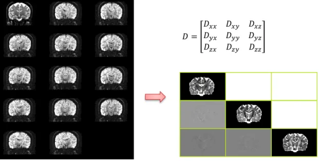
Basser et al., [3] introduced diffusion tensor magnetic resonance imaging (DT-MRI or DTI), which can be estimated from DWIs (Figure 1.1) under an assumption that molecular diffusion in tissues is Brown motion. A 3 × 3 symmetric and positive-definite matrix D
was called diffusion tensor (DT). DT can describe the main diffusivities λ1, λ2, λ3 (with
λ1 > λ2 > λ3) and the corresponding directions V1, V2, V3 of water diffusion.
Eigen-values λ1, λ2, λ3 can be combined to several scalar indices, such as relative anisotropy
(RA), fractional anisotropy (FA), and volume ratio (VR). Fractional anisotropy (FA) is the most commonly used index to characterize diffusion anisotropy. The range of FA is from 1 (anisotropic diffusion) to 0 (isotropic diffusion). The FA is defined as:
F A = q 3[(λ1− λ)2+ (λ2− λ)2+ (λ3 − λ)2] p2(λ2 1+ λ22+ λ23) (1.1)
1.2 Motivation 3
Figure 1.1: One slice of Diffusion tensor image (right) generated by diffusion-weighted images (left)
, where
λ = λ1+ λ2+ λ3
3 . (1.2)
1.2
Motivation
For subsequently statistical analysis and inter-subject brain comparison, spatial nor-malization was indispensable. Spatial nornor-malization is to transform each individual subject into the same stereotactic space, which is also called a brain template coordinate.
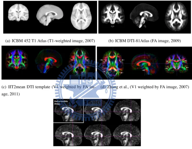
The well-known template spaces are Talairach atlas, MNI-305 and ICBM-152. Ta-lairach atlas [24] is based on dissection of a 60-year-old French females brain. It serves detailed anatomical labels. Montreal Neurological Institute (MNI) averaged 305 (MNI-305, [6, 7]) MR images. These 305 MR images were aligned to the Talairach atlas. ICBM-152 (Figure 1.2) is the current standard template. Before averaging the ICBM-152 western adult MR images, they were registered to MNI-305 by using a 9 parameter affine transform.
Several brain templates developed in ICBM-152 space, such as ICBM452 [20], ICBM DTI-81 atlas [19], IIT2 DT brain template [27] (Figure 3.6(a)(b)(c)(d)). However, Zilles
4 Introduction
Figure 1.2: ICBM 152 nonlinear atlases (version 2009)
et al., [28] confirmed that the brain structures are distinct from races. For example, the Japanese brains are shorter and wider than European brains. Furthermore, if a template has large variances from subjects, the large deformation may induce large distortion when subjects were registered. Hence, we want to provide a construction of the stereotactic space for a specific subject group. Namely, the template construction can be applied to different races, genders, ages, or diseases. There were some customized DTI brain template con-struction algorithms, such as Zhang et al., [26] and Goodlett et al., [9] (Figure 3.6(e)(f)). Zhang et al., [26] constructed an unbiased white matter atlas by using a piecewise affine al-gorithm to improve the accuracy of registration. They used traditional linear regression [3] to estimate tensor, and the tensor was calculated on Euclidean metrics. Goodlett et al., [9] proposed an unbiased atlas building for DTI population studies. The method they used in tensors estimation was based on the smoothed raw data [25]. Also, they applied Log-Euclidean metrics [2] (More detail in Section 2.2.6) on tensor calculation, such as inter-polation and averaging. Since the diffusion tensor is unsuitable to calculate in commonly Euclidean framework, we used the same strategy as Goodlett et al., on DTI calculation. Moreover, we chose an estimation tool to ensure the positive definiteness of all tensors, and the tool can tolerate the low SNR in clinical DWIs. All details of DTI processing were carefully considered in this study.
Additionally, we expect that this template space can reduce distortion from registration procedure. In order to increase the accuracy of registration, we considered the character
1.2 Motivation 5
(a) ICBM 452 T1 Atlas (T1-weighted image, 2007) (b) ICBM DTI-81Atlas (FA image, 2009)
(c) IIT2mean DTI template (V1 weighted by FA im-age, 2011)
(d) Zhang et al., (V1 weighted by FA image, 2007)
(e) Goodlett et al., (FA image, 2006)
Figure 1.3: (a),(b) and (c) were developed in the ICBM-152 space. (d) and (e) were cus-tomized DTI brain templates.
6 Introduction
of MR and DT images. In MR images, boundaries between different tissues can be well aligned by utilizing the information of intensity differences. However, it is difficult to ac-curately register the voxels within the same tissue solely relying on smoothness constraint. Castro et al., [5] assessed three MRI registration algorithms using the additional informa-tion carried out by DTI. They showed that the error increases with increasing FA value. That is, the accuracy of MRI registration in WM is lower than other tissues. Moreover, in DT images, different voxels have different diffusion tensors, which contain the diffusive direction, magnitude, and anisotropy of fibers. The information of DTI might be a remedy for registering WM voxels. Besides, the similarity of FA was commonly employed for non-rigid registration of DTI. Nevertheless, non-rigid registration of MRI performs better at the contours of tissues than FA. Hence, we proposed to register MR and DT images by simultaneously using both DT and MR information. As a consequence, the T1 and DTI templates were constructed by co-registering DT and MR images.
Chapter 2
8 Material and Methods
2.1
Materials
The MRI scans are obtained from Integrated Brain Research Unit (IBRU) of Taipei Veterans General Hospital. The MR images were acquired on a 1.5 Tesla GE MR scanner, using 3D-FSPGR pulse sequence (TR = 8.548 ms, TE = 1.836 ms, FOV = 260 × 260 × 1.5,
TI = 400 ms, NEX = 1, flip angle = 15◦, bandwidth = 15.63 kHz, matrix size = 256 × 256 ×
124, voxel size = 1.02 × 1.02 × 1.5); and diffusion weighted images (TR = 17000 ms, TE = 70.2 ms, FOV = 260 × 260 × 2.2, NEX = 6, matrix size = 128 × 128 × 70, voxel size =
2.03 × 2.03 × 2.2) consisted of 13 gradient directions with b = 900 s/mm2, and one b =
0 s/mm2 image. The subject group includes 20 males and 44 females in total 64 normal
subjects. Age range is from 21 to 62.
2.2
Methods
The purpose of our study is to create a template which can provide a stereotactic space for a subject group. Additionally, the subject images can be registered to this template space with little deformation. Hence, the goal is to minimize the variance between template and subject images. An adapted template construction and an accurate registration are needed. We modified the procedure of MRI template construction proposed by Lee [15] to construct our MRI and DTI templates. The new strategy of registration will be described in Section 2.3.
2.2.1
Template construction
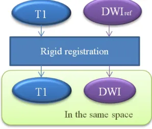
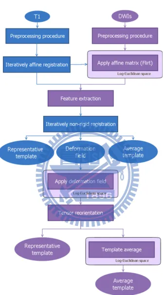
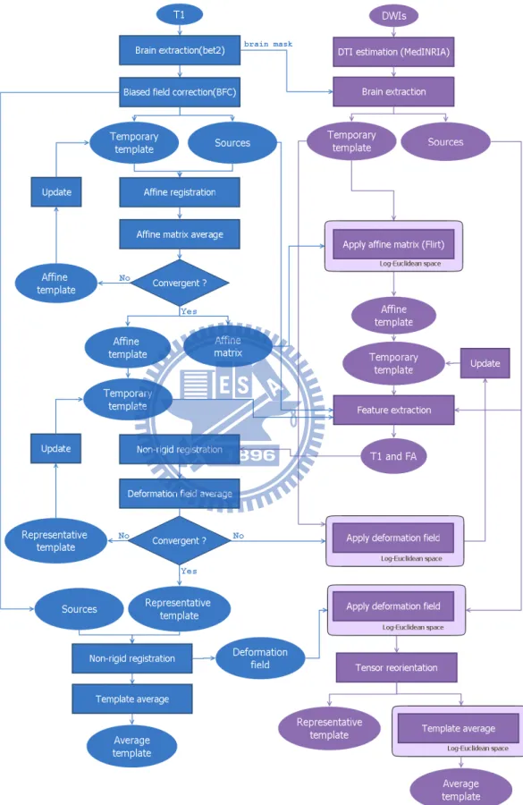
Figure 2.1, 2.2 and 2.3 illustrate our procedure for MR/DT template construction. The first step is to align MRI to the first volume (baseline image) of DWIs for each intra-subject by using rigid registration (Figure 2.1). It is to ensure that MRI and DWIs are in the same stereotactic space. The second step is the pre-processing for MRI and DWIs as described in Section 2.2.2.
To construct a customized template, an initial reference template R0is needed.
representa-2.2 Methods 9
Figure 2.1: Intra-subject alignment
tive subject had the smallest deformation magnitude kφk during registering this subject to other subjects. To find the representative subject, all possible pairs for registering a source image i to a target image j were considered. The equation can be expressed as follows:
R0 = arg min
i {kφi,j(x)k | ∀j 6= i, x ∈ brain coordinate} (2.1)
Note that, we only registered MR images to find the initial template, and directly as-signed the same representative subject of DT image as the initial template to reduce the calculus.
Following, the initial template was set as the temporary template (See Figure 2.3). each source image (of MRI) was registered to the temporary template of MRI. Each affine trans-formation will produce an affine matrix, which including four parameters: shearing, scal-ing, rotation, and translation. Then, we averaged the inverse of these four parameters from all affine matrices. Next, the average parameters were composed into an affine matrix. To avoid the temporary template will be blurred during iterations, the affine matrix was ap-plied on the representative subject instead of the temporary template. Finally, the affine result was set to the temporary template for next iteration. Repeated above step until the temporary template converges into a stable state (More detail about stopping criterion will describe in Section 2.2.4). As a consequence, an affine matrix and a correspondingly affine
10 Material and Methods
2.2 Methods 11
Figure 2.3: Detailed flowchart of the proposed methods for MR/DT template construction. Color blue and purple show the construction of MRI and DTI respectively.
12 Material and Methods
template of MRI were generated.
We utilized the affine matrix of MRI to co-register the initial template of DTI to the same template space. Subsequently, the features were extracted from preprocessed images and affine templates of both MRI and DTI. More detail about feature extraction and the new similarity function for non-rigid registration will describe in Section 2.2.3 and Section 2.2.4.
Iteratively affine transformation supplied the temporary template to iteratively non-rigid registration. Each source image was registered to the temporary template by two step: affine transformation and non-rigid registration. Affine transformation was a preliminary registration and it provided an affine matrix to non-rigid registration. Non-rigid registration generated a forward and an inverse deformation fields. In the similar way, the temporary template was updated by averaging the inverse deformation fields from each transforma-tion. Repeated these step until the template is convergent (More detail about stopping cri-terion will describe in Section 2.2.4). As a result, the deformation field and corresponding template (of MRI), called representative template, were created.
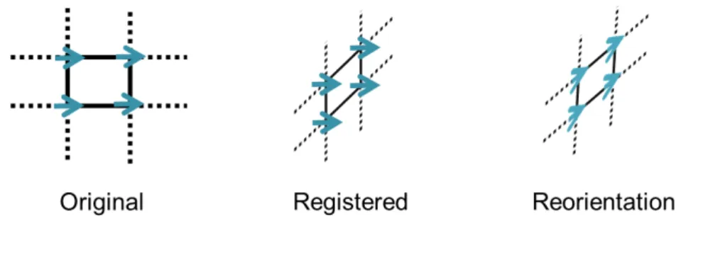
All subject images (of MRI) were registered to the representative template (of MRI). Finally, we averaged all registered subject images to create the average template (of MRI). The construction of DTI template is similar to MRI. The representative subject of DTI was co-registered to the same template space by using the deformation field of MRI. To maintain the property of DTI, the interpolation of DTI was computed in Log-Euclidean framework [2] (Section 2.2.6). Moreover, Figure 2.4 shows that after transformation, the position of voxels have been changed, but the direction have not. In order to maintain the consistency of the anatomical structure, tensor reorientation (Section 2.2.5) was applied. Then, the representative template of DTI was completed.
All subject images (of DTI) were co-registered to the representative template (of DTI) by using the deformation field of MRI. The average template of DTI was constructed by averaging the registered subject images as well. Nevertheless, we computed the average operators in Log-Euclidean space [2] (Section 2.2.6) instead of Euclidean space to avoid tensor swelling effect.
To summarize, we constructed four template: representative template and average tem-plate of both MRI and DTI. These temtem-plate are in the same stereotactic space, and they can
2.2 Methods 13
Figure 2.4: This diagram shows the tensor reorientation. Left : Four diffusive directions are located on the original stereotactic space. Mid : Four diffusive directions are located on the new stereotactic space after transformation. Right: Four diffusive directions are located on the new stereotactic space after transformation and tensor reorientation.
represent the subject group.
2.2.2
Preprocessing procedure
Preprocessing of MRI includes brain extraction and intensity inhomogeneity correction. We used Brain Extraction Tool (BET) version 2.1 [13, 23] and Bias Field Corrector (BFC) [22] to realize them separately.
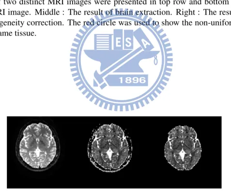
Brain extraction is to remove non-brain tissues, which will affect brain tissues registra-tion. Besides, brain extraction benefits to increase the accuracy of intensity inhomogeneity correction. Magnetic field inhomogeneity in MRI causes intensity non-uniformity. As-sume that a received image can be separate to two parts, which are an original image and a bias field. Bias field correction predicts a bias field and removes it to obtain the original image. The tool called BET has the additional value on intensity inhomogeneity correc-tion. Figure 2.5 indicates the non-uniform intensity was corrected after brain extraccorrec-tion. The non-uniform intensity will induce the error at image registration. For this reason, we applied BFC again for a further correction.
DWIs preprocessing includes DTI estimation and brain extraction as shown in Figure 2.6.
Fillard et al., [8] proposed a maximum likelihood strategy with Rician noise model to estimate diffusion tensor. In order to further reduce the influence of the noise, they
14 Material and Methods
Figure 2.5: This figure demonstrates each step of MRI preprocessing from left to right. One slice of two distinct MRI images were presented in top row and bottom row. Left : Original MRI image. Middle : The result of brain extraction. Right : The result of inten-sity inhomogeneity correction. The red circle was used to show the non-uniform inteninten-sity within the same tissue.
Figure 2.6: This figure demonstrates each step of DTI preprocessing from left to right. One slice of the first volume of DWIs and DTI images were presented. Left : Original DWIs image. Middle : Estimated DTI image. Right : The result of brain extraction.
2.2 Methods 15
combined estimation and regularization that results in a maximum a posteriori estimation. Moreover, the log-Euclidean metrics [2] (Section 2.2.6) was used to cancel the swelling effect in regularization. They developed a tool, called Medical Image Navigation and Re-search Tool by INRIA (MedINRIA), was used in our study to estimate the diffusion tensor. It can overcome the low SNR in clinical DWIs and ensure the positive definiteness of all tensors which are estimated from noise-sensitive DWIs.
Most brain extraction methods, such as BET, are designed for MRI. Little or no studies have ever tried to extract brain based on DWIs/DTI. For an accuracy result, we extracted the brain mask from the MR image and applied the mask on DTI instead of extracting brain region directly from DWIs or DTI.
2.2.3
Feature extraction
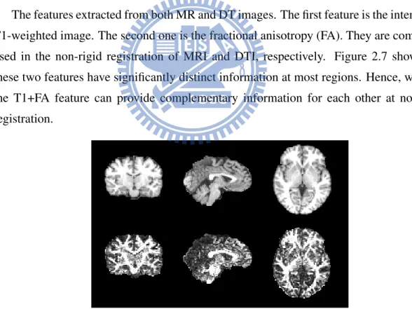
The features extracted from both MR and DT images. The first feature is the intensity of T1-weighted image. The second one is the fractional anisotropy (FA). They are commonly used in the non-rigid registration of MRI and DTI, respectively. Figure 2.7 shows that these two features have significantly distinct information at most regions. Hence, we hope the T1+FA feature can provide complementary information for each other at non-rigid registration.
Figure 2.7: This figure displays three different views of MRI (top row) and FA (bottom row) brain image. From left to right are coronal view, sagittal view and horizontal view.
16 Material and Methods
2.2.4
Image registration
Affine transformation
Affine transformation is a preliminary registration. It aligns the global shape from source image to target image. Here, FMRIB’s Linear Image Registration Tool (FLIRT) [11, 14] was used.
Non-rigid registration
Lin [16] proposed a non-rigid registration algorithm for MRI images. This algorithm supports two important properties for a custom template construction: diffeomorphic and symmetric (or inverse-consistency). To put it differently, the algorithm guarantees the map-ping function with smooth, invertible, and one-to-one relationship. In addition, if a trans-formation is generated by registering a source image to a target image, the unique inverse of the transformation will exactly register the target image to the source image.
Averaging the inverse deformation fields is an essential step in our iteratively non-rigid registration. In the previous construction proposed by Lee [15], the inverse of a transfor-mation is a critical issue because the non-rigid registration without the inverse-consistency property. The invertible can decrease the error may induce by estimating location and interpolation. Hence, the algorithm proposed by Lin [16] was employed in this work. Fur-thermore, we modified the similarity criterion to efficiently utilize the features extracted from DTI and MRI as mentioned. The new similarity evaluation function between target
image Itand source image Iscan be expressed as:
S(It, Is, Φ) = SCR(a
intensity
t , aintensitys , Φ) + SCR(aF At , aF As , Φ) (2.2) The similarity between target image and source image of the two features is assessed
by correlation ratio SCR [21]. More detail about correlation ratio describe in Section 2.2.4.
Because we want to improve the accuracy for non-rigid registration of both MRI and DTI, the influence of MRI and DTI is set as the same. For inverse-consistency, the equation can be rewritten as shown below.
2.2 Methods 17 S(It, Is, Φ) = S(Is, It, Φ−1) = SCR(aintensityt , a intensity s , Φ) + SCR(aF At , a F A s , Φ) + SCR(aintensitys , a intensity t , Φ −1) + S CR(aF As , a F A t , Φ −1) (2.3)
The correlation ratio SCR in Equation 2.3 had been normalized to the range of zero to
one. Large value indicates high image similarity. Hence, we maximized Equation 2.3 to obtain a better alignment.
Correlation ratio
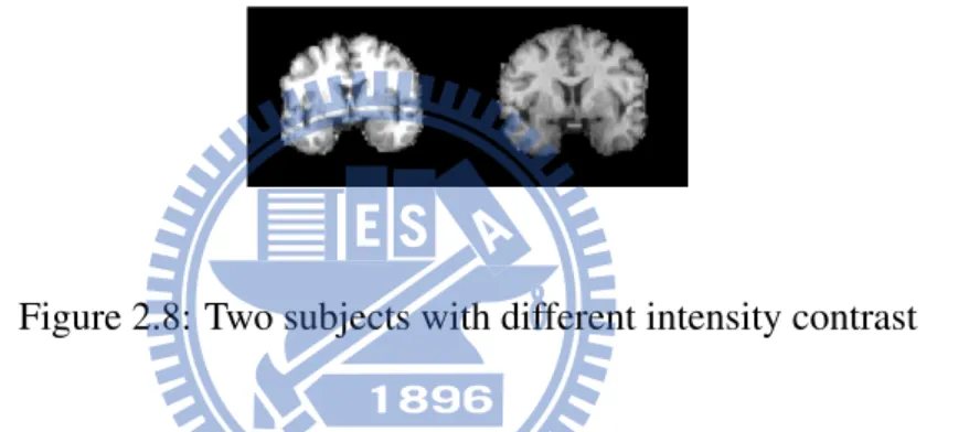
Figure 2.8: Two subjects with different intensity contrast
The correlation ratio is an efficiency and accuracy measurement for image registration. It is robust to different intensity contrast (See Figure 2.8), intensity inhomogeneity and noise [14, 21]. The correlation ratio on image similarity can be calculated by [17] (Figure 2.9): SCR(ait, a i s, Φ) = 1 − 1 V ar(ai s(Ω)) NB X j=1 Nj N V ar(a i s(Xj)) (2.4)
The range of features (intensity or FA) in target image was divided into NBbins. Voxels
in the same bin was gathered into a set Xj, which contains Nj voxels. We collected their
corresponding voxels in source image at set Xj, and calculated the variance from features
of these voxels. Let N be the number of voxels in the overlapping region Ω between source
image and target image. If the variance ratio of each set Xj to total volume Ω is small, the
18 Material and Methods
Figure 2.9: Correlation ratio
Stopping criterion
We used an iterative strategy to create a stable template in both affine and non-rigid registration. A stopping criterion proposed by Lee [15] is used. Since the registration will
not steady, if the difference between a new temporary template Ri+1 and last temporary
template Ri is small enough, it is called a stable state. For this reason, the slope IDP
(Equation 2.6) of intensity differences was compared to a threshold, α (Equation 2.7), for
stopping iterative registration. The intensity difference IDi between Ri and Ri+1 at each
voxel in brain volume Ω can be written as Equation 2.5.
IDi =X
v∈Ω
(Ri(v) − Ri+1(v))/Ω (2.5)
IDPi+1 = (IDi− IDi+1)/IDi (2.6)
If (IDPj < α) stop (2.7)
Outlier removing
Since the aim of our study is to create a stereotactic template for a subject group, the template should not be biased to any subject. Thus, if a subject image is registered to the
2.2 Methods 19
template with a larger deformation than other subjects, it would be considered as an outlier and would be removed from the template construction. We applied the strategy of outlier removing proposed by Lee [15] and replenished the outlier removing for DT image. First, the magnitude of shearing and scaling were examined when iteratively affine transforma-tion. Second, the magnitude of deform-only (not includes the deformation derived from affine transformation) along x, y, and z axes were inspected when iteratively non-rigid registration. Third, If a non-positive eigenvalue decomposed from a tensor of a subject, the subject would be set as an outlier. As a consequence, only the subjects passed these examinations can be constructed the average template.
2.2.5
DTI reorientation
Diffusion tensor contains direction of water diffusion in tissues. After affine transfor-mation, we only change position of voxels in DTI, but not direction. Likewise, non-rigid registering affects the orientation of the tissue structure. Therefore, we intend to maintain consistency of the anatomical structure by rotating each diffusion tensor according to the image transformation. Alexander et al., [1] developed a preservation of principal direction (PPD) method to estimate local rotation matrices from affine transformation or higher order transformations. The aim of PPD method is to preserve the principal direction and a plane spanned by principal direction and the second direction of a tensor after transformation. The PPD algorithm is:
• Step 1: Find the first eigenvector e1 and the second eigenvector e2 of a diffusion
tensor.
• Step 2: Compute the unit vectors n1 and n2from transformed e1 and e2, which were
applied by transformation matrix, F , respectively.
• Step 3: Rotate e1 to n1with rotation matrix, R1, and rotate e2with R1 as well.
• Step 4: Find a projection, P (n2), of n2onto a plane. The plane is spanned by n1and
n2, and it is perpendicular to n1. Besides, R1e2(rotate e2with R1) already lies in this
20 Material and Methods
• Step 5: Calculate the rotation matrix, R2, which maps R1e2 to P (n2).
• Step 6: Set the local rotation matrix R = R2R1 and reorient a tensor D by: D0 =
RDRT.
The transformation matrix F of higher order transformations, for instance a non-rigid transformation, is consists of an identity matrix I and the Jacobian matrix of displacement
field Φ by: F = I + JΦ.
2.2.6
Log-Euclidean metrics
Constructing average template of DTI is calculated in Euclidean space [2]. Log-Euclidean space can avoid the defects of Log-Euclidean calculus, such as tensor swelling effect and non-positive eigenvalues. Moreover, in this space, tensors can be looked upon as vec-tors. In other words, operations of vector can be used directly on tensors in Log-Euclidean space. Changing a tensor into Log-Euclidean space is as same as to calculate a matrix log-arithm of a tensor. Additionally, we can efficiently obtain the matrix loglog-arithm of a tensor by only three steps [2]:
• Step 1: D = RTM R • Step 2: M = λ1 0 0 0 λ2 0 0 0 λ3 −→ ˆM = logeλ1 0 0 0 logeλ2 0 0 0 logeλ3 • Step 3: log(D) = RTM Rˆ
Where M is a diagonal matrix with eigenvalues and R is a rotation matrix with eigen-vectors. They were factored from spectral decomposition of a tensor D. In contrast, chang-ing a tensor back into Euclidean space, that is, calculatchang-ing the matrix exponential of a tensor also can be obtained efficiently by using exponential substituted for logarithm at step 2. Moreover, to reduce the computations, the 3 × 3 symmetric matrix, log(D), can be represented by a 6D vectors as follows:
log(D) '−→D = (log(D)1,1, log(D)2,2, log(D)3,3,
√ 2 log(D)1,2, √ 2 log(D)1,3, √ 2 log(D)2,3)T (2.8)
2.2 Methods 21
Let N be the number of registered subject images and x be a voxel of tensor D, we obtained D(x) = exp " PN i=1log(Di(x)) N # (2.9) to construct our Average Template of DTI.
Besides, interpolation of tensors is also calculated in Log-Euclidean space. The prop-erties of tensors can be adequately maintained in Log-Euclidean space compared to in Euclidean space [2]. The interpolation with Log-Euclidean framework can be expressed as
D(x) = exp ( N X
i=1
wilog(Di(x))) (2.10)
, where wi is the trilinear weights.
2.2.7
Evaluation methods
Overlap index (OVL)
Basser and Pajevic [4] developed a measurement of tensor overlap based on eigenvalue-eigenvector pairs. If two different tensors are perfect match, the value of OVL is close to one. Conversely, the value is close to zero. The average overlap of a volume R, such as the region of white matter or brain region, was usually employed to evaluate the accuracy of DTI registration [10, 18]. The OVL and averaged OVL are given by:
OV L = P3 i=1λi(x)λ 0 i(x)(ei(x) · e 0 i(x))2 P3 i=1λi(x)λ 0 i(x) (2.11) Average OV L = 1 |R| X x∈R P3 i=1λi(x)λ 0 i(x)(ei(x) · e 0 i(x))2 P3 i=1λi(x)λ 0 i(x) (2.12) Error
Sanchez Castro et al., [5] utilized diffusion tensor images to evaluate MRI registration. They co-registered DTI with the transformation of MRI, and used the standard deviation,
22 Material and Methods
called error, to check the consistency of tensor after registration. They also performed operations on tensor in Log-Euclidean framework. The error can be computed as followed:
DLOG= exp( 1 N N X i=1 log(Di)) (2.13)
A = log(Di) − log(DLOG) (2.14)
ErrorDT I = v u u tT race( 1 N − 1 N X i=1 AAT) (2.15)
The error also can be applied to a specific volume by average each voxel in these
vol-ume. In our study, the error is computed for both MRI and DTI. In fact, DLOGis exactly
our Average Template of DTI. Similarly, registered subject images of MRI are averaged on Euclidean framework is the Average Template of MRI. In consequence, the error can rep-resent the discrepancy between our Average Template and registered subject images, and assists in evaluating the registration method we proposed. The MRI error can be expressed as follows: ErrorM RI = v u u t 1 N − 1 N X i=1 (T 1i− T 1)2 (2.16)
Chapter 3
24 Results and Discussion
Table 3.1: Mean OVL with average template in whole brain
Methods(features) OVL in whole brain ± Standard Deviation Affine transformation 0.606547 ± 0.038115
Non-rigid registration(T1) 0.589328 ± 0.038770 Non-rigid registration(FA) 0.617925 ± 0.026571 Non-rigid registration(T1+FA) 0.618822 ± 0.028180
The OVL measures the overlap of diffusion tensors in whole brain between DTI average template and registered DTI subjects.
Table 3.2: Mean OVL with average template in white matter
Methods(features) OVL in white matter ± Standard Deviation Affine transformation 0.779223 ± 0.077998
Non-rigid registration(T1) 0.775375 ± 0.078978 Non-rigid registration(FA) 0.815477 ± 0.042821 Non-rigid registration(T1+FA) 0.813633 ± 0.044007
The OVL measures the overlap of diffusion tensors in white matter between DTI average template and registered DTI subjects.
3.1
Feature comparison
In order to confirm the performance for the extracted features, MRI feature (T1 feature), DTI feature (FA feature) and the combination of them (T1+FA feature) were be considered. We compared the OVL in two cases: One is the tensor overlap between registered subjects and average template. The other is between registered subjects and representative template. In the average template case, Table 3.1 shows that T1+FA feature provides the highest OVL than other features in whole brain region. The second one is FA feature and the worst case is T1 feature. The effect upon distinct features in WM is more conspicuous than in whole brain (Table 3.2). Although the best one is FA feature in WM, the gap between FA feature and T1+FA feature is very small. In Table 3.1 and Table 3.2, the worst case is T1 feature. It is even worse than affine transformation in both whole brain and WM. In the representative template case, Table 3.3 and Table 3.4 display that affine transformation gives the highest OVL in both whole brain and WM. The OVL of T1+FA feature and T1 feature are comparable, and the lowest OVL is given by FA feature. However, we can found
3.1 Feature comparison 25
Table 3.3: Mean OVL with representative template in whole brain Methods(features) OVL in whole brain ± Standard Deviation Affine transformation 0.505459 ± 0.059662
Non-rigid registration(T1) 0.502208 ± 0.065645 Non-rigid registration(FA) 0.472313 ± 0.018574 Non-rigid registration(T1+FA) 0.502299 ± 0.025356
The OVL measures the overlap of diffusion tensors in whole brain between DTI representative template and registered DTI subjects.
Table 3.4: Mean OVL with representative template in white matter Methods(features) OVL in white matter ± Standard Deviation Affine transformation 0.588627 ± 0.068417
Non-rigid registration(T1) 0.587309 ± 0.072202 Non-rigid registration(FA) 0.545680 ± 0.023410 Non-rigid registration(T1+FA) 0.588053 ± 0.030262
The OVL measures the overlap of diffusion tensors in white matter between DTI representative template and registered DTI subjects.
that affine transformation and T1 feature supply high standard deviation (SD) of OVL in all regions and templates.
To summarize, T1+FA feature provides high OVL and low SD on both average template and representative template. FA feature provides high OVL and low SD only on average template. T1 feature provides high OVL but high SD on representative template. Although affine transformation provides high OVL on representative template and acceptable OVL on average template, it provides high SD on both cases. A good template should provide low SD to represent the subject group. Hence, the T1+FA feature is better than other methods.
Table 3.5 and Table 3.6 demonstrate the best reductions of DTI error are given by FA feature compared to affine transformation. T1+FA feature is the second in whole brain and WM, and it only has a slight gap between FA feature. A point is worth making about Table 3.6. The point is that T1 feature is worse than affine transformation in WM. It may because it is difficult to accurately register the voxels within the same tissue solely relying
26 Results and Discussion
Table 3.5: Mean ErrorDT I in whole brain
Methods(features) Average Error ± Standard Devi-ation
The reduction of error (%) com-pared to affine transformation Affine transformation 1.286436 ± 1.277231
Non-rigid registration(T1) 1.243496 ± 1.338124 3.34%±-0.05% Non-rigid registration(FA) 1.108207 ± 1.272015 13.85%±0.004% Non-rigid registration(T1+FA) 1.142485 ± 1.294859 11.19%±-0.01%
The DTI error checks the consistency of diffusion tensors in whole brain.
Table 3.6: Mean ErrorDT I in white matter
Methods(features) Average Error ± Standard Devi-ation
The reduction of error (%) com-pared to affine transformation Affine transformation 0.727660 ± 0.265835
Non-rigid registration (T1) 0.740338 ± 0.229792 -0.02%±13.56% Non-rigid registration (FA) 0.633133 ± 0.188424 12.99%±29.12% Non-rigid registration (T1+FA) 0.637518 ± 0.196857 12.39%±25.95%
The DTI error checks the consistency of diffusion tensors in white matter.
Table 3.7: Mean ErrorM RI in whole brain
Methods(features) Average Error ± Standard Devi-ation
The reduction of error (%) com-pared to affine transformation Affine transformation 109.891709 ± 47.428052
Non-rigid registration (T1) 76.489615 ± 30.807001 30.40%±35.04% Non-rigid registration (FA) 96.205667 ± 38.006380 12.45%±19.87% Non-rigid registration (T1+FA) 87.866330 ± 36.887101 20.04%±22.23%
3.1 Feature comparison 27
Table 3.8: Mean ErrorM RI in white matter
Methods(features) Average Error ± Standard Devi-ation
The reduction of error (%) com-pared to affine transformation Affine transformation 86.905587 ± 32.754628
Non-rigid registration (T1) 62.531859 ± 11.482740 28.05%±64.94% Non-rigid registration (FA) 77.624157 ± 22.972671 10.68%±29.86% Non-rigid registration (T1+FA) 69.362197 ± 23.376631 20.19%±28.63%
The MRI error shows the difference of T1 images in white matter.
on smoothness constraint.
Table 3.7 and Table 3.8 display that T1 feature obtains the best reduction of MRI error compared to affine transformation. The second is still T1+FA feature and the third is FA feature. To summarize, T1+FA feature and FA feature are comparable in DTI error and OVL. Besides, T1+FA feature gives an acceptable result in MRI error. Hence, we can find that T1 and DTI can provide the complementary effect.
Let us examine OVL and errors in more detail. As showed in Figure 3.1 and Figure 3.2, these evaluation methods were partitioned into ten part by using FA image, which was derived from DTI Average Template. Figure 3.2(a) shows that FA feature provides the best error reduction of DTI in major divisions. However, T1+FA feature is better than FA feature when FA being the range between 0.7 and 0.9. T1 feature gives the terrible errors especially when FA=0.3∼0.5. Furthermore, Figure 3.1(a) displays that T1+FA feature, T1 feature and affine transformation are comparable. Also, T1+FA feature supplied higher OVL than others when FA=0.7∼0.9. Figure 3.1(b) shows that the OVL of FA feature and T1+FA feature are higher than others. Although T1+FA feature was not perfect in each detail segment, it also provided a competent performance.
There are sufficient evidence to prove that T1 feature performs well at MRI error and provides poor performance in DTI error. FA feature is contrary to T1 feature. It may be-cause T1 feature leads accuracy alignment in tissue boundaries but not inside the same tissues, and FA feature characters the anisotropy of tissues but not the tissue boundaries. Moreover, the range of FA is from zero to one, and the value of FA in white matter is
gener-28 Results and Discussion
ally larger than 0.3. That is, the information for gray matter and other tissues which tend to isotropy are fewer than white matter region. These findings lead us to believe that T1 fea-ture and FA feafea-ture should be simultaneously used in non-rigid registration. Excitingly, the results demonstrate that T1 and FA can provide complementary information for each other when they are simultaneously employed in non-rigid registration. Accordingly, T1+FA feature supplies the competent alignment for both MRI and DTI non-rigid registration.
(a) (b)
Figure 3.1: Mean OVL with different features (a) The OVL between registered subjects and representative template (b) The OVL between registered subjects and average template
3.2
Curve analysis
Whether which feature was used in non-rigid registration, the results of DTI error, MRI error, and OVL were displayed specific trends.
In DTI error case (See Figure 3.2(a)), we can found that the error was very high when FA value tends to zero. A possible reason is that when FA value tends to zero, the water diffusion tends to isotropy. That is to say, the diffusive direction is not along a particular direction in a tissue with isotropy. Namely, the eigenvectors of these tissues are very differ-ent, and the DTI is generated by eigenvalue-eigenvector pairs. As a consequence, the DTI
3.2 Curve analysis 29
(a) (b)
30 Results and Discussion
error should be high when FA value tends to zero. Another phenomenon we can observe in Figure 3.2(a) is that the error increased with FA value when FA value was bigger than 0.3. A possible reason is that the water diffusion tend to anisotropy when FA value is more and more large. Hence, a little misalign and individual differences may induce large DTI error. Figure 3.2(b) demonstrates that the MRI error increases with decreases in FA value. A probable reason is that the boundaries of different tissues usually have lower FA value. In addition, the MRI Average Template is more fuzzier than other subjects. For these reason, the boundaries of tissues may lead to larger MRI error than other regions.
It is reasonable to see that the OVL increases with FA value increases in Figure 3.1. However, the OVL of affine transformation is higher than non-rigid registration when FA=0.8∼0.9 (Figure 3.1(b)). It may be caused that the number of voxels increased with the increase of FA value after non-rigid registration (See Figure 3.3). Since the FA bin was divided by Average Template of DTI, the phenomenon represents that more registered subject images have high FA value in the same voxel. Namely, the non-rigid registration is more accurate than the affine transformation particularly in FA feature and T1+FA feature cases. The number of voxel of FA/T1+FA feature is much higher than affine transforma-tion/T1 feature when FA value is high. Furthermore, FA/T1+FA feature lead to a high OVL in high FA bin. It indicates that the non-rigid registration of FA/T1+FA feature is accurate.
3.3
Framework comparision
The interpolation of DTI in Euclidean framework caused non-positive eigenvalues. The non-positive eigenvalues was illogical in physical and it led to large DTI error and its stan-dard deviation (See Table 3.9). For this reason, Log-Euclidean framework is a better choice for calculating tensors than Euclidean framework.
3.4
Average template and representative template
Figure 3.4 and 3.5 are the representative template and average template constructed by the present procedure in this study. The DTI template is a six volumes image. For
visual-3.4 Average template and representative template 31
Figure 3.3: Number of voxels with average template in different FA value bins
Table 3.9: Mean ErrorDT I in whole brain
Methods (Framework) Average Error ± Standard Deviation Affine (Log) and Average (Log) 1.286436 ± 1.277231
Affine (Euclidean) and Average (Log) 1.957571 ± 2.349731 Affine (Euclidean) and Average (Euclidean) 2.548714 ± 3.623380 Non-rigid (Log) and Average (Log) 1.142485 ± 1.294859 Non-rigid (Euclidean) and Average (Log) 1.652078 ± 2.449258 Non-rigid (Euclidean) and Average (Euclidean) 2.053583 ± 3.736114
32 Results and Discussion
Table 3.10: Cross-correlation between template and subjects Template Mean correlation ± Standard Deviation Average template 0.974866 ± 0.004335
Representative template 0.9543609 ± 0.003394317
ization, we used FSLView [12]. In Figure 3.4(b) and Figure 3.5(c)(d), the first eigenvector (V1) is modulated by FA to represent the principal diffusion direction and its magnitude (where the colors red, green, and blue represent diffusion in the x, y, and z axes respec-tively). We can find that the average templates are sharper than the averages of affine subjects from both MRI and DTI. Additionally, the detailed structure of average templates consists with the representative templates of both MRI and DTI.
As show in Table 3.10, the correlations present a strong relationship between templates (of MRI) and registered subjects, especially with average template. Table 3.11 illustrates the OVL between average template (of DTI) and registered subject image is higher than the case of representative template (of DTI). Particularly in WM region, the OVL is significant high. Because the representative template should bias to the initial subject, the correlation and OVL are lesser than average template. Even so, representative template still provides acceptable correlation and OVL.
To summarize, we constructed four template in the same stereotactic space for a specific subject group. The average templates of both MRI and DTI can provide the information of all subjects, and the representative template of both MRI and DTI can characterize the detail structure for the subject group. In order to provide the relationship between our tem-plates and the standard stereotactic space (ICBM-152 space). We normalized our temtem-plates to ICBM-152 space by registering the templates to ICBM452 atlas. Figure 3.6 displays the corresponding templates in the standard stereotactic space and the reference template (Fig-ure 3.6(a)).
3.5 Comparison with different DTI template construction 33
Table 3.11: Mean OVL between average template and subjects Template Mean OVL ± Standard Deviation Average template 0.618822 ± 0.028180 Average template (WM) 0.813633 ± 0.044007 Representative template 0.502299 ± 0.025356 Representative template (WM) 0.588053 ± 0.030262 (a) (b)
34 Results and Discussion
(a)
(b)
(c)
(d)
Figure 3.5: (a) Average template of MRI (b) Average template of affine MRI(c) Average template of affine DTI (d) Average template of DTI
3.5 Comparison with different DTI template construction 35
(a) ICBM452 atlas
(b) Representative template of MRI (c) Average template of MRI
(d) Representative template of DTI (FA image) (e) Average template of DTI (FA image)
(f) Representative template of DTI (V1 weighted by FA image)
(g) Average template of DTI (V1 weighted by FA im-age)
36 Results and Discussion T able 3.12: Comparison with dif ferent DTI template construction Our method IIT2 (Zhang et al., 2011 ) [27] ICBM (Mori et al., 2008 ) [19] Zhang et al., (2007) [26] Goodlett et al., (2006) [9] Institute NCTU & NYMU (T aiw an) Illinois Institute (USA) Uni v ersity of Cali-fornia Los Angeles (USA) Uni v ersity of Penn-sylv ania (USA) Uni v ersity of North Carolina (USA) Number of subjects 64 (61) 67 81 13 5 Age 21-62 20-40 18-59 -1 Dif fusion directions 13+1 12+2 30+1 15+1 6+1 T ar get image Customized ICBM152 ICBM152 Customized Customized DTI estimation MedINRIA FSL-DTIFIT DtiStudio Linear re gression [3] W estin’ s method [25] Af fine method Flirt AR T AIR -Non-rigid method The proposed DTIGUI AIR Piece wise Af fine al-gorithm [26] Goodlett’ s method [9] T emplate av erage Log-Euclidean Euclidean Euclidean Euclidean Log-Euclidean Interpolation Log-Euclidean Euclidean Euclidean Euclidean Log-Euclidean Reorientation Euclidean Euclidean Euclidean Euclidean Euclidean -: not mentioned
3.5 Comparison with different DTI template construction 37
3.5
Comparison with different DTI template construction
Table 3.12 lists the comparison between our procedure and other DTI template con-structions [27] [19] [26] [9]. Although the concept of Log-Euclidean metrics has been published in 2006 [2], it did not commonly used in DTI template construction. One expla-nation for this is that the theory of most estimation methods are based on high SNR and large number of gradient directions. However, in clinical, the number of gradient directions is limited and noise-sensitive DWIs is low SNR. These properties of DWIs may cause zero eigenvalues or negative eigenvalues when estimate tensors by most estimation methods. Nevertheless, non-positive eigenvalues cannot be explained in biological tissues. Besides, non-positive eigenvalues cannot be accepted by logarithmic transformation, which is an es-sential step in changing a tensor into Log-Euclidean space. Hence, we used MedINRIA [8] to confirm the positive definiteness of all tensors, in other words, zero eigenvalues and negative eigenvalues would not be derived from the spectral decomposition of estimated tensors.
However, the good property of tensors cannot always maintain in tensor calculus. Es-pecially when we calculate tensors in Euclidean space, it may occur non-positive eigenval-ues and tensor swelling effect, which is mean that the determinant of a calculated tensor in Euclidean space will larger than its original determinant. Hence, in this study, we used Log-Euclidean framework to calculate tensors, such as interpolation and average of tensors. Nonetheless, we applied the the tensor reorientation in Euclidean framework. Because PPD
method applied the rotation matrix to a tensor (D0 = RDRT) in the final step, and it only
affect on direction but not magnitude of a tensor.
An advantage of our study is the outlier removing scheme. If the number of subjects is not few, the outlier removing scheme is necessary for a customized template construction. It because the custom template should not bias to outliers, which are very different from other subjects. In our study, the number of subjects is 64 before template construction. Fi-nally, three outliers were removed in the removing scheme. Figure 3.7 shows a comparison between Average Template of MRI and outliers. The first outlier was removed by the large scale of shearing along z-axis at iterative affine transformation. The second one and the last one were removed by the large deformation along y-axis at iterative non-rigid
registra-38 Results and Discussion
tion. We can found that no subject was removed by the non-positive eigenvalue detection. Accordingly, we can affirm that all DTI processes were suitable to maintain the property of diffusion tensors.
(a) (b)
(c) (d)
Figure 3.7: (a) Average Template of MRI. (b) removed at iterative affine transformation. (c) and (d) removed at iterative non-rigid registration.
Chapter 4
Conclusions
40 Conclusions
4.1
Conclusions
In this study, we present a procedure to construct MRI and DTI templates in the same stereotactic space. Since the diffusion tensor is unsuitable to calculate in commonly Eu-clidean framework, all details of DTI processing procedure were carefully considered. First, a satisfactory tool of tensor estimation was chosen to ensure the positive definite-ness of all tensors and tolerate the low SNR in clinical DWIs. Second, interpolation and average of tensors were computed with Log-Euclidean metrics to avoid the problem of tensor swelling effect and non-positive eigenvalues. Finally, the DTI reorientation method was applied in Euclidean framework to maintain the consistency of the anatomical structure after transformation.
Additionally, we improved the accuracy of registration procedure to reduce the distor-tion during the template construcdistor-tion procedure. A symmetric and diffeomorphic non-rigid registration algorithm was used to solve the issue of estimating inverse transformation. Moreover, we proposed an objective function which can simultaneously utilize the both MRI and DTI features to improve the accuracy of registration. Furthermore, the results displayed a high correlation between the proposed template and registered subject images. To summarize, the brain template construction could provide a stereotactic space for a specific subject group by using MRI and DTI data. Also, we provided the relationship be-tween our templates and the standard stereotactic space to facilitate subsequently statistical analysis.
4.2
Future works
In this study, the number of subjects is 64 including 44 females and 20 males. In the future, we will collect more subjects to balance the distribution of gender. Moreover, we will apply the template construction for different specific subject groups to provide the stereotactic spaces.
In this study, we only applied FA feature to assist the non-rigid registration due to preserve the efficiency. Moreover, using diffusive direction or other features which can be derived from DTI might increase the accuracy in non-rigid registration. Hence, an area of
4.2 Future works 41
Bibliography
[1] D.C. Alexander, C. Pierpaoli, P.J. Basser, and J.C. Gee. Spatial transformations of diffusion tensor magnetic resonance images. IEEE Transactions on Medical Imaging, 20(11):1131–1139, 2001.
[2] V. Arsigny, P. Fillard, X. Pennec, and N. Ayache. Log-euclidean metrics for fast and simple calculus on diffusion tensors. Magnetic Resonance in Medicine, 56(2):411– 421, 2006.
[3] P.J. Basser, J. Mattiello, and D. LEBiHAN. Estimation of the effective self-diffusion tensor from the nmr spin echo. Journal of Magnetic Resonance Series B, 103:247– 247, 1994.
[4] P.J. Basser and S. Pajevic. Statistical artifacts in diffusion tensor mri (dtmri) caused by background noise. Magnetic resonance in medicine, 44(1):41–50, 2000.
[5] F. J. S. Castro, O. Clatz, J. Dauguet, N. Archip, J. Ph Thiran, and S. K. Warfield. Evaluation of brain image nonrigid registration algorithms based on log-euclidean mr-dti consistency measures. In Biomedical Imaging: From Nano to Macro, 2007. ISBI 2007. 4th IEEE International Symposium on, pages 45–48.
[6] D.L. Collins, P. Neelin, T.M. Peters, and A.C. Evans. Automatic 3d intersubject reg-istration of mr volumetric data in standardized talairach space. Journal of computer assisted tomography, 18(2):192, 1994.
[7] A.C. Evans, D.L. Collins, SR Mills, ED Brown, RL Kelly, and TM Peters. 3d statis-tical neuroanatomical models from 305 mri volumes. pages 1813–1817 vol. 3. IEEE.
44 BIBLIOGRAPHY
[8] P. Fillard, X. Pennec, V. Arsigny, and N. Ayache. Clinical dt-mri estimation, smooth-ing, and fiber tracking with log-euclidean metrics. IEEE Transactions on Medical Imaging, 26(11):1472–1482, 2007.
[9] C. Goodlett, B. Davis, R. Jean, J. Gilmore, and G. Gerig. Improved correspondence for dti population studies via unbiased atlas building. Medical Image Computing and Computer-Assisted Intervention MICCAI 2006, pages 260–267, 2006.
[10] M. Ingalhalikar, J. Yang, C. Davatzikos, and R. Verma. Dtidroid: Diffusion tensor imagingdeformable registration using orientation and intensity descriptors. Interna-tional Journal of Imaging Systems and Technology, 20(2):99–107, 2010.
[11] M. Jenkinson, P. Bannister, M. Brady, and S. Smith. Improved optimization for the robust and accurate linear registration and motion correction of brain images. Neu-roImage, 17(2):825–841, 2002.
[12] M. Jenkinson, C.F. Beckmann, T.E.J. Behrens, M.W. Woolrich, and S.M. Smith. Fsl. NeuroImage, 62(2):782–790, 2012.
[13] M. Jenkinson, M. Pechaud, and S. Smith. Bet2: Mr-based estimation of brain, skull and scalp surfaces. pages 12–16.
[14] M. Jenkinson and S. Smith. A global optimisation method for robust affine registra-tion of brain images. Medical Image Analysis, 5(2):143–156, 2001.
[15] Kuo-Wei Lee. Construction of customized brain template from magnetic resonance images. Master’s thesis, 2011.
[16] Shih-Yen Lin. A fast and accurate algorithm for diffeomorphic and symmetric non-rigid registrations of brain magnetic resonance images. Master’s thesis, 2012.
[17] Jia-Xiu Liu. Brain Extraction and Registration Algorithms for Computational
Anatomy. PhD thesis, 2009.
[18] Chiang Ming-Chang, A. D. Leow, A. D. Klunder, R. A. Dutton, M. Barysheva, S. E. Rose, K. L. McMahon, G. I. de Zubicaray, A. W. Toga, and P. M. Thompson. Fluid
BIBLIOGRAPHY 45
registration of diffusion tensor images using information theory. IEEE Transactions on Medical Imaging, 27(4):442–456, 2008.
[19] S. Mori, K. Oishi, H. Jiang, L. Jiang, X. Li, K. Akhter, K. Hua, A.V. Faria, A. Mah-mood, and R. Woods. Stereotaxic white matter atlas based on diffusion tensor imaging in an icbm template. NeuroImage, 40(2):570–582, 2008.
[20] D.E. Rex, J.Q. Ma, and A.W. Toga. The loni pipeline processing environment. Neu-roImage, 19(3):1033–1048, 2003.
[21] A. Roche, G. Malandain, X. Pennec, and N. Ayache. The correlation ratio as a new similarity measure for multimodal image registration. Medical Image Computing and Computer-Assisted Interventation MICCAI98, pages 1115–1124, 1998.
[22] D.W. Shattuck, S.R. Sandor-Leahy, K.A. Schaper, D.A. Rottenberg, and R.M. Leahy. Magnetic resonance image tissue classification using a partial volume model. Neu-roImage, 13(5):856–876, 2001.
[23] S.M. Smith. Fast robust automated brain extraction. Human Brain Mapping,
17(3):143–155, 2002.
[24] J. Talairach and P. Tournoux. Co-planar stereotaxic atlas of the human brain: 3-dimensional proportional system: an approach to cerebral imaging. Thieme, 1988.
[25] C.F. Westin, SE Maier, H. Mamata, A. Nabavi, FA Jolesz, and R. Kikinis. Processing and visualization for diffusion tensor mri. Medical Image Analysis, 6(2):93–108, 2002.
[26] H. Zhang, P.A. Yushkevich, D. Rueckert, and J.C. Gee. Unbiased white matter atlas construction using diffusion tensor images. pages 211–218. Springer-Verlag.
[27] S. Zhang, H. Peng, R.J. Dawe, and K. Arfanakis. Enhanced icbm diffusion tensor template of the human brain. NeuroImage, 54(2):974–984, 2011.
46 BIBLIOGRAPHY
[28] K. Zilles, R. Kawashima, A. Dabringhaus, H. Fukuda, and T. Schormann. Hemi-spheric shape of european and japanese brains: 3-d mri analysis of intersubject vari-ability, ethnical, and gender differences. NeuroImage, 13(2):262–271, 2001.