國
立
交
通
大
學
統計學研究所
碩
士
論
文
使用模擬資料來比較選取標籤單體核苷酸多樣性、
分單體型區塊與相關性檢定所用不同方法之
組合
Comparison of Combinations of SNP Tagging,
Haplotype Blocking and Association Testing
Using Simulated Data
研 究 生:林煜淳
指導教授:黃冠華 博士
使用模擬資料來比較選取標籤單體核苷酸多樣性、
分單體型區塊與相關性檢定所用不同方法之
組合
Comparison of Combinations of SNP Tagging,
Haplotype Blocking and Association Testing
Using Simulated Data
研 究 生:林煜淳 Student:You-Chun Lin
指導教授:黃冠華 Advisor:Dr. Guan-Hua Huang
國 立 交 通 大 學
統計學研究所
碩 士 論 文
A Thesis
Submitted to institute of Statistics College of Science
National Chiao Tung University in Partial Fulfillment of the Requirements
for the Degree of Master
in Statistics July 2007
Hsinchu, Taiwan, Republic of China
Comparison of Combinations of SNP Tagging,
Haplotype Blocking and Association Testing Using
Simulated Data
Student :You-Chun Lin Advisor:Guan-Hua Huang
Institute of Statistics
National Chiao Tung University
ABSTRACT
Population association studies with case-control designs are powerful to detect the genetic variations responsible for human common diseases. We were interested in how the tag SNP selection methods with association tests and samples used for tag SNP discovery would have on power. We used four methods for choosing tag SNPs: three based on haplotype diversity, one based on pair-wise linkage disequilibrium (LD) and four methods to detect association: three based on multiple-SNP test, one based on single-SNP test. Besides, haplotype blocking is an important factor we considered. In two regions from the Genetic Analysis Workshop 15 simulated data, we estimated the power and type I error at each match. The multiple-SNP test is more power than single-SNP test. In most situations, the case sample used for tag SNP selection is more power than the control sample. Association sample sizes are evident reason to effect power but tag SNP selection sample sizes are not significant to power. At the end, we advised some combinations of methods for SNP analysis.
使用模擬資料來比較選取標籤單體核苷酸多樣性、分
單體型區塊與相關性檢定所用不同方法之組合
研究生 : 林煜淳
指導教授 : 黃冠華 博士
國立交通大學統計學研究所
摘要
使用病例-對照研究方法的母群體相關性檢定對於偵測人類一般疾病的治病 基因有顯著功效,我們感興趣的是比較不同選取標籤單體核苷酸多態性的方法與 不同相關性檢定方法在不同樣本下的檢定力。 我們使用四種選取標籤單體核苷酸多態性方法,其中三種方法是基於單體型 多樣性,一種是基於兩兩連鎖不平衡的觀點;並選用四種相關性檢定的方法,其 中三種是基於多重單體核苷酸多態性,一種是基於單一單體核苷酸多態性的觀 點,此外,分單體型區塊的方法也是我們考慮的一項因素。 我們從一組名為「第十五次基因分析專題討論模擬資料」中選出兩段區域來 估計每種方法的檢定力與型一錯誤。 相關性檢定中,使用多重單體核苷酸多態性的方法會比使用單一單體核苷酸 多態性的方法具有較高的檢定力,且在做標籤單體核苷酸多態性時選用疾病樣本 會比選用非疾病樣本有較高的檢定力。 樣本大小是影響相關性檢定的檢定力之重要因素,但對於做標籤單體核苷酸 多態性時並不會有顯著的影響,最後我們建議了幾種在做單體核苷酸多態性時較 好的方法組合。 關鍵字 :單體核苷酸多態性、母群體相關性檢定、標籤單體核苷酸多態性、 單體型、連鎖不平衡誌謝
這兩年體驗了研究生的生活讓我覺得非常充實,學了很多東西但可能也忘了 不少,很開心能夠畢業了,能夠把論文寫出來還真的有點小小驕傲。 要感謝的人很多,先謝謝辛苦的老師,不時的給我建議並修改我不像英文的 英文讓我能順利寫出論文,還有幫助我程式的吸血雪芳、益銘、建威等等,還要 感謝雅莉跟素梅,在大家都口試過後我們留下來一起共患難到最後,再來還要感 謝和我一起吃吃喝喝,打球,打電動的好同學 : 建威、俊睿、益銘、阿 Q、永 在、育辰、益通,還要感謝家人,讓我每次回到家時都能很放鬆,儲備電力後在 回新竹努力。 最後以本論文獻給所有我的師長,同學,朋友,獻上我最大的謝意。 林煜淳 2007/7/6Content
Abstract
i
摘要
ii
誌謝 i i i
Tables
and
Figures
Content
v
1. Introduction
1
2. Literature review
4
2.1 SNP ……… 4 2.2 Haplotype ……… 5 2.2.1 Haplotype frequencies ……… 6 2.3 Linkage disequilibrium ……… 6 2.4 Tag SNP ………..……… 92.4.1 Methods based on haplotype distribution ……… 10
2.4.2 Methods based on pairwise LD ……… 12
2.5 Tests of association ……… 13
2.5.1 Single SNP ……… 13
2.5.2 Multiple SNPs ……… 13
3. Materials
and
methods
15
3.1 Study population ……… 15
3.2 Study design ……… 16
3.3 SNP tagging methods ……… 19
3.4 Association study methods ……… 20
4. Results
21
5. Conclusion
28
Tables and Figures Content
Table 1.
Values are number of tag SNPs divided total number of SNPs, average from 100 replication selecting tag SNPs in blocks and not in blocks .25Table 2.
Values are number of tagging SNPs divided total number of SNPs,and average from 100 replication selecting tagSNPs in blocks …...25
Table 3.
Association sample = 500cases-500controls in casual region ...…29Table 4.
Association sample = 200cases-200controls in casual region ...…30Table 5.
Association sample = 500cases-500controls in null region ……… 31Table 6.
Association sample = 500cases-500controls in casual region .……32Figure 1.
The design of the whole study, (a) tag SNP selection (b) association s study ……….18Figure 2.
LD plot used 1500 cases and 1500 controls, CI-blocking in low LD region ………22Figure 3.
LD plot used 1500 cases and 1500 controls, CI-blocking in low LD region ………22Figure 4.
LD plot used 1500 cases and 1500 control data SSLD-blocking in low LD region ………. 23Figure 5.
LD plot used 1500 cases and 1500 control data SSLD-blocking in high LD region ……….23Figure 6.
power of tagger – association methods ………33Figure 7.
power of haplotype+CI – association methods ………... 34Figure 8.
power of haplotype+SSLD – association methods ………. 35Figure 9.
power of haplotype+1-Block – association methods ……….. 36Figure 10.
power of haplotype+CI – association methods in (2) situation ...….371
Introduction
Population association studies with case-control designs are powerful in detecting the genetic variations responsible for human common diseases and are increasingly used in epidemiological studies. Single nucleotide polymorphism (SNP) markers are preferred for association studies because of their high abundance along the human genome, low mutation rate and the accessibility of high-throughput genotyping [1-2]. Population association studies can be classified into two different types: the candidate gene approach focuses on typing 5-50 SNPs within a gene hypothesized to be responsible for the studied disease, whereas the genome-wide approach seeks to identify the common causal variants throughout the genome and requires more than 300,000 well-chosen SNPs [3]. This report intends to compare various analytic combinations in performing the candidate-gene association studies.
SNPs within the candidate gene can be identified from publicly available databases (e.g., NCBI dbSNP (http://www.ncbi.nlm.nih.gov/projects/SNP/), Inter- national HapMap project (http://www.hapmap.org/)). To reduce genotyping costs, tagging SNP methods have been developed. Tagging refers methods to select a minimal number of SNPs that retain as much as possible of the genetic variation of the full SNP set [3]. Tagging SNP methods are used to select a “good” subset of SNPs (tag SNPs) to be typed in all the study individuals from an extensive SNP set that has been typed in just a few individuals [3]. Criteria such as pairwise linkage disequilibrium (LD) and haplotype diversity can be used to determine tag SNPs. Obtaining samples with genotypes on the full SNP set from sources such as the International HapMap project for tag SNP discovery can save both time and costs. However, tag SNPs selected in the population for which public data are available might perform poorly in the population underling a particular study.
To test for association between tag SNP genotypes and case-control status, we can analyze one SNP at a time or multiple SNPs jointly. The single-SNP tests can neglect information in the joint distribution of tag SNPs, whereas the multiple-SNP tests might loss of power due to the introduction of additional statistical tests [4]. Also, the most efficient association test will depend on the tagging strategy used.
When using haplotype-diversity criterion for selecting tag SNPs or performing multiple-SNP association tests, haplotype data are needed. Direct laboratory -haplotyping is an expensive way to obtain haplotypes. Fortunately, there are statistical methods for inferring haplotypes from the genotypes of unrelated individuals. The inference process can be very accurate when there is very little recombination between the SNPs [5]. Thus, to be effective, tag SNP selection and multiple-SNP association tests must be undertaken within “haplotype blocks” covering much of the genome over which there is little evidence for recombination [5]. To define blocks, Gabriel et al. [6] used 95% confidence bounds on D’ (a measure of pairwise LD) and Haploview software [7] searched for a “spine” of strong LD to.
After identifying haplotype blocks, haplotype-based SNP tagging and association testing are performed on the SNPs within blocks. The question is what should be done about SNPs that fall outside haplotype blocks. For selecting tag SNPs, two approaches can be used. The first approach includes all SNPs outside blocks as part of the tag SNP set to retain more genetic variation of the full SNP set. On the contrary, the second approach excludes them all because studies indicate that these SNPs are hotspots of chromosomal recombination separating haplotype blocks [5] and are rarely the genetic variants underlying common diseases (the common-disease common- variant hypothesis). The second approach results in less tag SNPs. However, if the common-disease common-variant hypothesis is in doubt or if the block
define by the population underlying the study, the power gained by using the first approach may be large. Before performing multiple-SNP association tests on selected tag SNPs, the block boundaries of tag SNPs are re-defined by all study objects. To determine whether tag SNPs are disease loci, each tag SNP outside the re-defined haplotype blocks is test for association, together with results from multiple-SNP tests within haplotype blocks [3].
The present study considered pairwise-LD/haplotype-diversity criteria for SNP tagging, confidence-interval/spine-of-strong-LD block definitions, and single/multiple-SNP association tests. We estimated the power and type I error of selected tag SNPs to detect association over 100 simulated case-control studies and compared the number of tag SNPs selected. We were also interested in the effects of various samples used for tag SNP discovery, different approaches handing SNPs outside haplotype blocks and the sample sizes in association tests.
2
Literature review
2.1
SNP (
http://en.wikipedia.org/wiki/Single_nucleotide_polymorphism)
A Single Nucleotide Polymorphism or SNP is a DNA sequence variation occurring when a single nucleotide A, T, C, or G in the genome (or other shared sequence) differs between members of a species (or between paired chromosomes in an individual). For example, two sequenced DNA fragments from different individuals, AAGCCTA to AAGCTTA, contain a difference in a single nucleotide. In this case we say that there are two alleles : C and T. Almost all common SNP have only two alleles.
Within a population, SNPs can be assigned a minor allele frequency- the ratio of chromosomes in the population carrying the less common variant to those with the more common variant. Usually one will want to refer to SNPs with a minor allele frequency of ≥ 1% (or 0.5% etc.). It is important to note that there are variations between human populations, so a SNP is common enough for inclusion in one ethnic group may be much rarer in another.
SNPs may fall within coding sequences of genes, noncoding regions of genes, or in the intergenic regions between genes. SNPs within a coding sequence will not necessarily change the amino acid sequence of the protein that is produced, due to degeneracy of the genetic code. A SNP in which both forms lead to the same polypeptide sequence is termed synonymous (sometimes called a silent mutation) - if a different polypeptide sequence is produced they are non-synonymous. SNPs that are not in protein coding regions may still have consequences for gene splicing, transcription factor binding, or the sequence of non-coding RNA.
Variations in the DNA sequences of humans can affect how humans develop diseases and respond to pathogens, chemicals, drugs, etc. However, their greatest
importance in biomedical research is for comparing regions of the genome between cohorts (such as cohorts with and without a disease). Technologies from Affymetrix and Illumina allow for genotyping hundreds of thousands of SNPs for typically under $1,000.00 in a couple of days.
2.2
Haplotype (
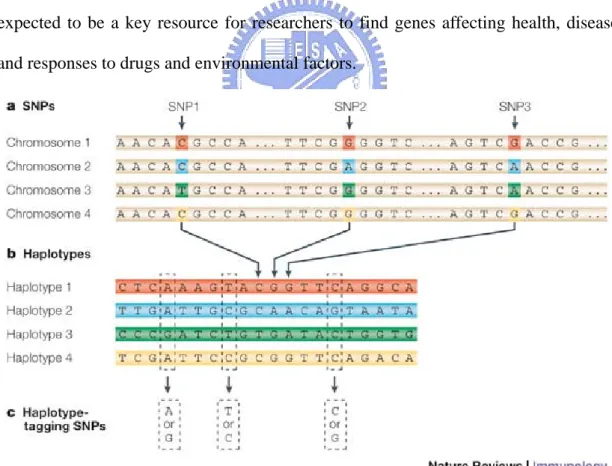
http://www.hapmap.org/)Haplotype is a set of SNPs on a single chromatid that is statistically associated. It is thought that these associations, and the identification of a few alleles of a haplotype block, can unambiguously identify all other polymorphic sites in its region. Such information is very valuable for investigating the genetics behind common diseases and is collected by the International HapMap Project. The HapMap Project is expected to be a key resource for researchers to find genes affecting health, disease and responses to drugs and environmental factors.
Figure : The construction of the HapMap occurs in three steps. (a) Single nucleotide polymorphisms (SNPs) are identified in DNA samples from multiple individuals. (b) Adjacent SNPs that are inherited together are compiled into "haplotypes." (c) "Tag"
SNPs within haplotypes are identified that uniquely identify those haplotypes. By genotyping the three tag SNPs shown in this figure, researchers can identify which of the four haplotypes shown here are present in each individual.
2.2.1 Haplotype frequencies
One can use the EM algorithm to estimate haplotype frequency. The likelihood of the haplotype frequencies is 1 2 1 1 1 1 2 1
,
,
)
(
(
)
)
1
(
− = =−
−
−
−
=
=
∏ ∑
m h h j n c i il ik ha
p
h
h
where
p
p
p
p
p
p
p
L
j j…
…
1a is a constant incorporating the multinomial coefficient
m is different phenotypes and its observed with counts n1,n2,…,nm
j
c is the number of genotypes
p(hkhl) is the probability of the i genotype made up of haplotypes k and l th
The EM algorithm is an iterative method to compute successive sets of haplotype frequencies P1,P2,…Ph, start with initial arbitrary values
) 0 ( ) 0 ( 2 ) 0 ( 1 ,P , Ph P … these
initial values are used as if they were the unknown true frequencies to estimate genotype frequencies P(hkhl)(0)(the expectation step )These expected genotype frequencies are used in turn to estimate haplotype frequencies at the next iteration
) 1 ( ) 1 ( 2 ) 1 ( 1 ,P , ,Ph
P … (the maximization step), and so on until convergence is reached.
2.3
Linkage disequilibrium
(http://en.wikipedia.org/wiki/Linkage_disequilibrium)
Linkage disequilibrium is a term used in the study of population genetics for the non-random association of alleles at two or more loci, not necessarily on the same
chromosome. It is not the same as linkage, which describes the association of two or more loci on a chromosome with limited recombination between them. Linkage disequilibrium describes a situation in which some combinations of alleles or genetic markers occur more or less frequently in a population than would be expected from a random formation of haplotypes from alleles based on their frequencies. Non-random associations between genes at different loci are measured by the degree of linkage disequilibrium.
Linkage disequilibrium is generally caused by interactions between genes, genetic linkage and the rate of recombination, random drift or non-random mating and population structure. For example, some organisms may show linkage disequilibrium (such as bacteria) because they reproduce asexually and there is no recombination to break down the linkage disequilibrium.
If inspecting the two loci A and B with two alleles each (i.e., a two-locus, two-allele model), the following table denotes the frequencies of each combination:
Haplotype Frequency
A1 B1 x11
A1 B2 x12
A2 B1 x21
A2 B2 x22
A common convention is to set A1, B1 to be the common allele and A2, B2 to be the
Allele Frequency A1 p1 = x11 + x12
A2 p2 = x21 + x22
B1 q1 = x11 + x21
B2 q2 = x12 + x22
If the two loci and the alleles are independent from each other, then one can express the observation A1B1 as "A1 must be found and B1 must be found". The table above lists the frequencies for A1, p1, and B1, q1, hence the frequency of A1B1, x11, equals
according to the rules of elementary statistics x11= p1×q1.
A deviation of the observed frequencies from the expected is referred to as the linkage disequilibrium parameter, introduced by Robbins [8] and named by Lewontin and Kojima [9] and commonly denoted by a capital D as defined by D=x11− p1q1. It is vividly presented in the following table.
A1 A2 Total
B1 x11 = p1q1+ D x21 = p2q1− D q1
B2 x12 = p1q2−D x22 = p2q2 + D q2
Total p1 p2 1
D is nice to calculate with but has the disadvantage of depending on the frequency of the alleles inspected. This is evident since frequencies are between 0 and 1. There can be no D observed if any locus has an allele frequency 0 or 1 and is maximal when frequencies are at 0.5. Lewontin [10] suggested normalising D by dividing it with the theoretical maximum for the observed allele frequencies. Thus,
max D
D
⎪⎩
⎪
⎨
⎧
=
′
< > 0 ) , min( 0 ) , min( 2 2 1 1 2 1 2 1 D q p q p D D p q q p DD
Another value is the correlation coefficient. Let I1 and I2 be the indictors of
alleles at two loci. The square of the correlation coefficient between I1 and I2 is
denoted as 2 2 1 1 2 2 2 1 2 1 2 ) var( ) var( ) , cov( q p q p D I I I I r ⎟⎟ = ⎠ ⎞ ⎜ ⎜ ⎝ ⎛ = .
This however is not adjusted to the loci having different allele frequencies.
2.4
Tag SNP (
http://en.wikipedia.org/wiki/Tag_SNP)
A tag SNP is representative single nucleotide polymorphisms (SNPs) in a region of the genome with high linkage disequilibrium. It is possible to identify genetic variation without genotyping every SNP in a chromosomal region. Tag SNPs are significant in whole-genome SNP association studies which hundreds of thousands of SNPs across the entire genome are genotyped. For this reason, the HapMap Project hopes to use tag SNPs to discover genes responsible for certain disorders.
To deal with the issue of genotyping costs, SNP tagging methods have been developed. In regions of high LD, where many SNPs are frequently inherited together and thus highly correlated within populations, it may not be necessary to genotype all of the SNPs in a given region to capture all of the genetic information. In fact, it would be wasteful to do so. A reduced set of SNPs can be representative of most, if not all, genetic variation in that region. The goal of SNP tagging methods is to determine which SNPs to include in this reduced set.
haplotype + 1-Block and used one pairwise-LD-based method: tagger.
2.4.1 Methods based on haplotype distribution
The method identifies the set of markers that best captures the haplotype information. The selection is based on statistics related to diversity criteria: the proportion of haplotype diversity explained by the tag SNPs and the residual diversity, measuring how well these tag SNPs can predict the markers excluded from the set. For a given number of tag SNPs, the best subset is the one that best maximizes the overall percentage of haplotype diversity observed while minimizing the residual diversity. The number of tag SNPs to keep is then determined by comparing the diversity values of best subset of each size. The smallest subset that scores well the different statistics will be the one finally chosen.
We know that there will be limited haplotype diversity in each block, thus only a few kinds of common haplotypes can account for a bulk percentage of population. The measurement of haplotype diversity becomes an important subject. Diversity is defined as d =1-
∑
(xi)2, where xi represents the frequency of this kind of haplotypewithin the block, and n represents the number of distinct types of haplotype. ⇓ ⇓ 1 2 3 4 5 6 7 8 9 10 H1 0 0 1 0 1 1 0 1 1 1 H2 0 0 0 0 1 1 0 1 1 0 H3 0 0 1 1 1 0 1 1 0 1 H4 0 1 0 1 0 1 1 1 0 1
It is an example of four haplotypes where two SNPs (tag SNPs) are sufficient to identify each of four haplotypes. Three are many ways to choose tag SNPs, and
different results are allowed.
Haplotype block partitioning and tag SNP selection
There are many methods have been developed for block partitioning and SNP tagging cased on haplotype data. These methods can be classified into two categories. Haplotype blocks are first obtained based on a pairwise LD pattern [6], a four-gamete test [11]. Tag SNPs are then selected in each resulting block. In the second group, the goal is to minimize the total number of tag SNPs over a region of interest or whole genome [12-13].
Haplotype blocks are used as a tool to achieve the objective. The algorithms developed in Patil et al. [12] and Zhang et al. [13] can only be applied to haplotype data. In this paper, we follow the first category of methods, and express how to select tag SNPs in a block fixed.
Tag SNPs in a block are selected to minimize the number of SNPs that can distinguish at least α percent of all the observed haplotypes.
Consider a matrix, P, containing i = 1,…, N haplotypes (rows) and t = 1, . . . T markers(columns) .
1. For all pairs of haplotypes I and j (i <>j), set aij(t) =1 if the allele at marker t
differs between i and j. 2. ⎩ ⎨ ⎧ = otherwise 0 set SNP tagging in the included is marker t if 1 ) (t x 3. Minimise
∑
t tx
( ) subject to the constraint∑
≥
t
t t
ij
x
a
( ) ()1
for all pairs i andj (i<>j). A minimum number of tag SNPs needs for any tag SNP set is calculated as follows: for m haplotypes find the minimum n satifying 2n ≥m. A set recovery process is then employed to produce tag SNPs sets with n or more tag SNPs. For each tag SNP set, the haplotype diversity captured is measured: if the
set uniquely identifies two haplotypes, the tag SNP set’s diversity score is incremented by one. This measurement terminates at any time if the set fails to identify any pair of haplotypes.
2.4.2 Methods based on pairwise LD
The method relies on linkage disequilibrium and more specifically on r , the squared 2 stardized coefficient. At first, bins of SNPs are defined by grouping together SNPs with r value that exceed a chosen threshold. All the SNPs within a same bin are not 2 necessarily in strong LD since if SNP A exceeds the r threshold with SNP B. 2 And SNP C, this might be untrue for the pair SNP B/SNP C. The markers exceeding the r threshold with all the markers of the bin are the ones designated as tag SNP. 2 Several tag SNPs may be designated within a same bin and in second step, the user can then refine the selection using different criteria. The tag SNP can be selected for assay on the basis of genomic context (coding vs. noncoding or repeat vs. unique), ease of assay design, or other user-specified criteria. The binning process is iterated, analyzing all as-yet-unbinned SNPs at each round, until all sites are binned. Each bin is reported as a set of all SNPs in the bin as well as the subset of tag SNPs within the bin, each of which is above the r threshold with all other SNPs in the bin. If a SNP 2 does not exceed the r threshold with any other SNP in the region, it is placed in a 2 singleton bin.
For example, suppose there was a bin with SNP A, B, C and D and A had
2
r -value 0.83, 0.81, 0.82 with B, C, D, respectively. Similarly ,B had r -value 2 0.83,0.82,0.83 with A,C,D;C had r -value 0.81,0.82,0.79 with A,B,D; and D had 2
2
r -value 0.82,0.83,0.79,with A,B, and C. If r^2 threshold were0.80, SNP A and B would be selected as alternative tag SNPs for the bin. The average r of A with the 2
B could be regarded as a better tag than A and was output first
2.5
Tests of association
Estimating the power of the selected subsets was to detect an association using single SNP tests and multiple SNPs tests. In this paper we only considered population association studies in which unrelated individuals of different disease states are typed at a number of SNP markers. We did not consider family-based association studies or linkage studies, which also have an important role in efforts to understand the effects of genes on disease [14].
2.5.1 Single SNP
The most natural analysis of SNP genotypes and case-control status at a single SNP is to test the null hypothesis of no association between rows and columns of the 2×3
matrix that contains the counts of the three genotypes among cases and controls. For complex traits, it is widely thought that contributions to disease risk from individual SNPs will often be roughly additive-that is, the heterozygote risk will be intermediate between the two homozygote risks. One way to improve power to detect additive risks is to count alleles rather than genotypes so that each individual contributes 2× 2 table and a Pearson 1-df test can be applied [14].
2.5.2 Multiple SNPs
There were L SNPs genotyped in cases and controls at a candidate gene that is subject to little recombination or an LD-block within a gene, we might want to decide whether or not the gene is associated with the disease. A popular method, suggested by the block structure of the human genome, is using haplotypes to capture the correlation structure of SNPs in regions of little recombination. Haplotypes can
capture the combined effects of tightly linked cis-cating causal variants. Given haplotype assignments, the simplest analysis involves testing for independence of rows and columns in a 2× table, where k denotes the number of distinct k haplotypes [14].
3
Materials and methods
3.1
Study population
The Genetic Analysis Workshop 15 simulated dataset was used for this study (http://www.gaworkshop.org/welcome.html). The plan for this simulated dataset was to mimic the familial pattern of rheumatoid arthritis (RA) including a strong effect of DR type at the HLA locus on chr6 and other genetic and environmental effects. For each of 100 replicates, they generated a large population of above two million nuclear families (two parents and two offspring) with RA affection status determined by a complex genetic/environmental model, then they retained a random sample of 1500 families from those families that had an effected sibling pair (ASP) and a random sample of 2000 families where none of the four members were affected (control). They present markers on 22 autosomes which were designed to be like real human autosomes in terms of genetic and physical map lengths. These markers are in three sets:
1. A set of 730 microsatellite markers, fairly evenly spaced on chromosomes with an average inter-marker distance of above 5 CM and with heterozygosities always exceeding 0.7.
2. A set of 9187 SNPs distributed on genome to mimic a 10K SNP chip set but without monomorphic SNPs.
3. A very dense map of 17820 SNPs on chromosome 6 (an average interval marker spacing of 9586 bp which corresponds roughly to the density one would expect from a genome-wide 300K SNP set). The chromosome 6 dense map includes 210 of the markers from the 10K SNP map (they are easily identifiable because they have the same names in both sets).
selected one causal region on chromosome 6 between 37070499 bp and 37338545 bp, which was known to contain a disease locus D. Besides, we chose another null region on chromosome 6 between 50001131 bp and 50341279 bp, which was far from locus D and did not contain any disease loci. We considered all 30 dense SNP markers in the causal region and 30 dense SNP markers in the null region.
3.2
Study design
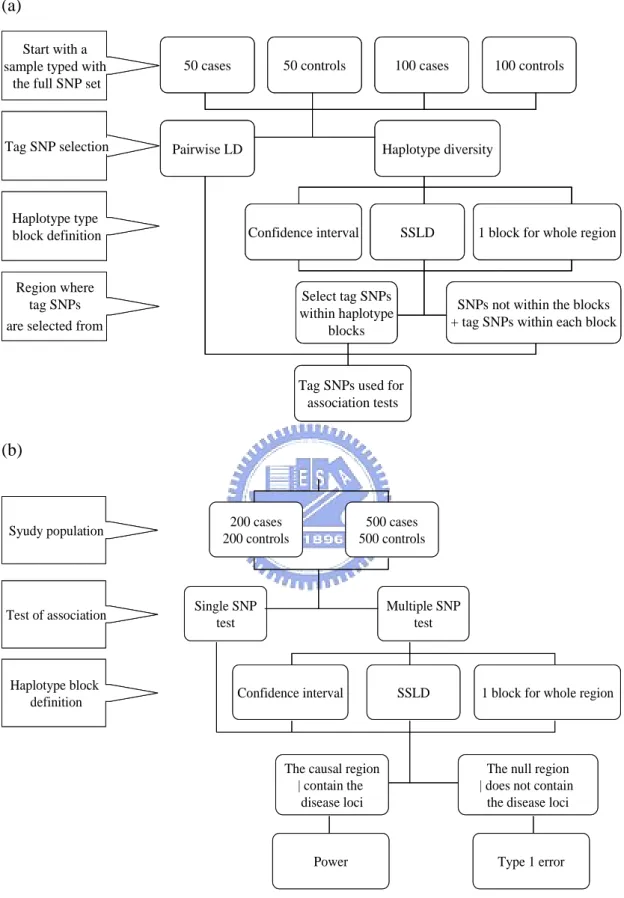
The design of the whole study is show in Figure 1. For tag SNP selection, we randomly selected 50 cases, 50 controls, 100 cases and 100 controls from the entire population. After tag SNP selection, we performed case/control association tests using either 200 cases and 200 controls, or 500 cases and 500 controls. Individuals from the tag SNP selection step were also included in the association study.
Four combinations of tag SNP criteria and block definitions were used to select tag SNPs: pairwise LD implemented in Tagger software (tagger), haplotype diversity with blocking according to the confidence interval of D′ (haplotype+CI), haplotype diversity with blocking according to the spine of strong LD (haplotype+SSLD), and haplotype diversity with the whole region as one block (haplotype+1-block). When using haplotype+CI and haplotype+SSLD, haplotype diversity criterion is for finding tag SNPs within identified haplotype blocks. For SNPs falling outside haplotype blocks, we either included them all as part of the tag SNP set or excluded them all.
To test the association between SNP genotypes and disease phenotypes, we considered four various tests: single-SNP test (single-SNP), multiple-SNP test (multi-SNP) with blocking according to the confidence interval of D′ (multi-SNP + CI), multiple-SNP test with blocking according to the spine of strong LD (multi-SNP + SSLD), and multiple-SNP test with the whole region as one block (multi-SNP +
sample for tag SNP discovery, while the haplotype blocks for multiple-SNP association tests were determined by the entire population.
Detailed option setting under each tagging and association methods can be found in the following section.
(a)
50 cases 50 controls 100 cases 100 controls
Pairwise LD Haplotype diversity
Confidence interval SSLD 1 block for whole region
Select tag SNPs within haplotype
blocks
SNPs not within the blocks + tag SNPs within each block
Tag SNPs used for association tests Start with a
sample typed with the full SNP set
Tag SNP selection
Haplotype type block definition
Region where tag SNPs are selected from
50 cases 50 controls 100 cases 100 controls
Pairwise LD Haplotype diversity
Confidence interval SSLD 1 block for whole region
Select tag SNPs within haplotype
blocks
SNPs not within the blocks + tag SNPs within each block
Tag SNPs used for association tests
50 cases 50 controls 100 cases 100 controls
Pairwise LD Haplotype diversity
Confidence interval SSLD 1 block for whole region
Select tag SNPs within haplotype
blocks
SNPs not within the blocks + tag SNPs within each block
Tag SNPs used for association tests Start with a
sample typed with the full SNP set
Tag SNP selection
Haplotype type block definition
Region where tag SNPs are selected from
(b)
Power Type 1 error 200 cases 200 controls 500 cases 500 controls Single SNP test Multiple SNP test
Confidence interval SSLD 1 block for whole region
The causal region | contain the
disease loci
The null region | does not contain
the disease loci Syudy population
Test of association
Haplotype block definition
3.3
SNP tagging methods
tagger. Tagger is a tool for the selection and evaluation of tag SNPs from genotype data. It combines the simplicity of pairwise tagging methods with the efficiency benefits of multi-marker haplotype approaches. In tagger, bins of SNPs are defined across a region according to pairwise LD. Bins of SNPs are created based on the specified r threshold, then one SNP is selected to represent the remainder of SNPs 2 in that bin . In this study, we used an r threshold of 0.8 and minimum allele 2 frequency of 0.05.
haplotype + CI. The history of recombination between a pair of SNPs can be estimated with the use of the normalized measure of allelic association, D' Because D' values are known to fluctuate upward when a small number of samples or rare alleles are examined, we relied on confidence bounds on D' rather than point estimates
In this tag SNP selection method, LD blocks are first defined according to method of Gabriel et al [6] and SNPs that represent the underlying haplotypes are chosen within blocks. Pairs of SNPs are defined as having “strong evidence for historical recombination” if the upper confidence bound on D’ is less than 0.9 , and a block is defined as a region over which less than 5% of SNP pairs show strong evidence of historical recombination . Tagging SNPs are then selected per block as a set of SNPs which define all haplotypes above a given frequency threshold >1%.
Haplotype + SSLD. This method used the SSLD algorithm to define blocks by searching for a “spine” of LD, such that the first and last markers in a block are in strong LD with all intermediate markers. We recognized it is strong LD by D’>0.8. However the intermediate markers are not necessarily in LD with each other. Tagging SNPs are then selected per block to define all haplotype > 1% frequency.
Haplotype + 1-Block. This approach selects regard from an entire region of interest, without regard to LD blocks, so we let 30 SNPs to be a haplotype region. Tagging
SNPs are selected based on the ability of any SNP subset to maintain the overall haplotype diversity observed when considering SNPs. Then we selected tagging SNPs based on the haplotype frequency >1%.
3.4
Association
study methods
Single-SNP test. Single-locus tests of association between SNP allele frequencies and case-control status were carried out via standard contingency x tests and P values 2 were determined via x approximation. It should be noted that for demonstration 2 purposes, we have considered the α = 0.05 / (the number of tag snps) type 1 error rate to report significance.
Multiple-SNP test. The haplotype-based hypothesis test focused on the differences in individual haplotype frequencies between the case and control groups. The x 2 statistics were derived from a series of simple 2 by 2 tables based on the frequency of each haplotype versus all others combined between the case and control groups. We have considered the α = 0.05 / (the number of haplotypes + the number of tagSNPs outside blocks) type 1 error rate to report significance. We also selected three blocking methods to do haplotype association method only using SNPs be tagged.
4.
Results
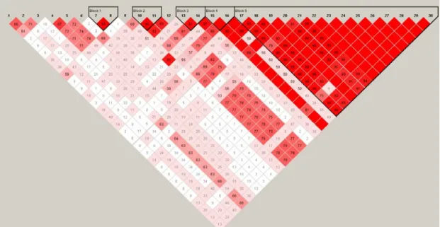
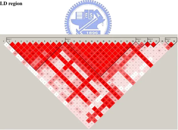
The two region of total of 30 SNPs we selected , first region contain the disease locus D length about 260 kb and the other is away from locus D its length about 340 kb. Locus D has a direct effect on RA risk but a low allele frequency. Distance between the two regions is above 12662 Kb, 27 CM (centi-Morgan).With this distance we can say the null region can not affect the disease. Our goal was getting power from the causal region to see which match is the best and the null region can get type 1 error to compare. We note that if the method has the large power in the causal region and less power in the null region, we can say it is the best method we want to select. First we used the character of pair-wise LD plot to understand different of the two regions and difference number of tag SNPs using the four methods. We used the Haploview software to get the pair-wise LD plot, and show the four LD plots of the two regions in Figure 2 to 5.
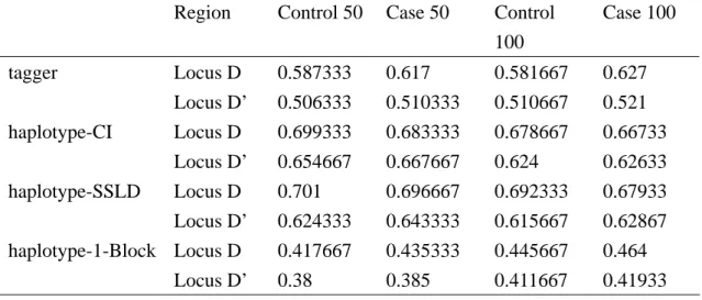
The color was more deep and the LD more high. We saw that the second region (Figure 3, Figure 5) has high LD than first region (Figure 2, Figure 4), and it would effects the proportions of tag SNPs selected from 30 SNPs. The proportions of tag SNPs selected have no difference between the four samples sizes for each of 4 tagSNP’s methods (Table 1, Table 2). Here we considered two situations in methods of hapotype + CI and haplotype+SSLD. The idea of first situation is in terms of tag SNPs, the two methods of tag SNPs haplotype+CI and haplotype+SSLD selected tag SNPs in blocks and all remaining SNPs outside of blocks (Table 1). Second idea is in terms of association that selected tag SNPs only in blocks (Table 2). The first situation was certain to have more tag SNPs than second, but whether it was useful we would analysis later.
Figure 2. LD plot used 1500 cases and 1500 controls, CI-blocking in low LD region
Figure 3. LD plot used 1500 cases and 1500 control data CI-blocking in high LD region
Figure 4. LD plot used 1500 cases and 1500 control data SSLD-blocking in low LD region
Figure 5. LD plot used 1500 cases and 1500 control data SSLD-blocking in high LD region
All methods of tag SNP have more SNPs in the causal region than the null region in first situation. The reason is the causal region having low levels of pair-wise LD than the null region. But in second situation, method of haplotype+CI has adverse result because blocks in high LD become large and having more SNPs (Figure 2, Figure 3). As a result of haplotype+SSLD that selected almost all SNPs as tag SNPs, so it still has high proportion of tag SNPs in high LD region (Figure 4, Figure 5).
In first situation, the methods as tagger and haplotype+1-Block has fewer markers than the methods as haplotype+CI and haplotype+SSLD, possible they were not restricted to full representation of each LD block. And the two methods, haplotype+CI and haplotype+SSLD almost have the same number of tag SNPs (Table 1). In second situation, haplotype+CI has the least number of tag SNPs, because tag SNPs were selected only in blocks and the block sizes of haplotype+CI is smaller than haplotype+SSLD (Table 2).
We can see the two methods of haplotype+1-Block and haplotype+CI selected the less tag SNPs. If using these methods to do analysis can use less costs. But whether these methods have the same power to detect disease is the next step we want to do.
The goal of our study was to compare different combinations of SNP tagging methods and association methods on a simulation dataset to select the best match. First we selected a random sample of 50 individuals from one of an affected sibling pair from 1500 families, and 50 individuals from unaffected 2000 families. Then we used the same way to select a subject of 100 case and 100 controls. The methods of tag SNP used these four samples to analysis.
Table 1. Values are number of tag SNPs divided total number of SNPs, and average from 100 replication selecting tag SNPs in blocks and not in blocks.
Region Control 50 Case 50 Control 100 Case 100 tagger Locus D 0.587333 0.617 0.581667 0.627 Locus D’ 0.506333 0.510333 0.510667 0.521 haplotype-CI Locus D 0.699333 0.683333 0.678667 0.66733 Locus D’ 0.654667 0.667667 0.624 0.62633 haplotype-SSLD Locus D 0.701 0.696667 0.692333 0.67933 Locus D’ 0.624333 0.643333 0.615667 0.62867 haplotype-1-Block Locus D 0.417667 0.435333 0.445667 0.464 Locus D’ 0.38 0.385 0.411667 0.41933
Table 2. Values are number of tagging SNPs divided total number of SNPs, and average from 100 replication selecting tagSNPs in blocks.
Region Control 50 Case 50 Control 100 Case 100 tagger Locus D 0.587333 0.617 0.581667 0.627 Locus D’ 0.506333 0.510333 0.510667 0.521 haplotype-CI Locus D 0.299333 0.259 0.310333 0.25267 Locus D’ 0.384667 0.384667 0.413 0.421 haplotype-SSLD Locus D 0.632333 0.638 0.613 0.60433 Locus D’ 0.548667 0.569333 0.534667 0.54833 haplotype-1-Block Locus D 0.417667 0.435333 0.445667 0.464 Locus D’ 0.38 0.385 0.411667 0.41933
Second we did association study by using a mix subject from sample of 500 cases and 500 controls random from populations. Another subject is from 200 case sand 200 controls. The reason was that we want to understand whether association sample sizes would affect the power of detecting disease. Further when doing haplotype association study we used three blocking methods, Gabriel blocking, SSLD
blocking and third is using 1 block for all region. Then we defined Bonferroni-corrected p-value let α 0.05 / (the number of haplotypes + the number = of tag SNPs outside blocks) as using the multi-SNP test; α 0.05 / (the number of = tag SNPs) as using the single-SNP test. Then we used 100 repeated random samples and estimated power with the proportion of replicates having p-value less than type 1 error. Result Show in Table 3 to 6.
When doing tag SNP methods there was no significant difference using sample size of 50 or 100 in the same Tag-Association match and powers have almost the same degree. So we thought that sample size of 50 or 100 we selected would not affect the result of power. Samples size of 50 was enough to achieve our goal to decide which Tag-Association match methods was better. But it still should be depend on the complicacy of disease gene.
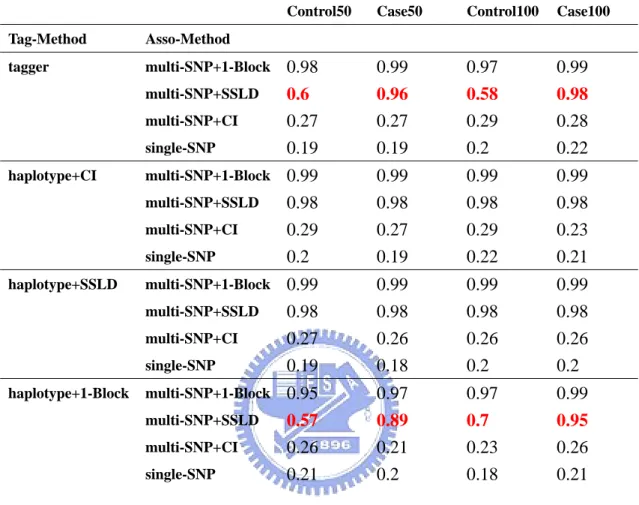
We divided two situations when we selected tag SNPs for methods of haplotype+CI and haplotype+SSLD. Then we advanced some common points in the two situations. In association methods the three multi-SNP methods, multi-SNP+1-Block, multi-SNP+SSLD and multi-SNP+CI have large power then the single association test methods. It have biggish gap between multi-SNP+1-Block, multi-SNP+SSLD and single-SNP test. Although multi-SNP+CI did not have such large gap like multi-SNP+1-Block or multi-SNP+SSLD, it still was a little bigger than single-SNP test. From this we though that the method of multiple SNPs test was a powerful reason to affect the level of power. And in multiple SNPs test the approach of blocking was important. There was no difference between the two situations using haplotype+SSLD in four samples of tag SNP. It was a consistence method.
there were two significant differences at the combination of tagger and multi-SNP+SSLD and at the combination of haplotype+1-Block and multi-SNP+SSLD. They had large power in case and the difference about 30 % to 40 % (Table 3.a). We reduced the association sample sizes to 200 cases-200 controls, we found that tagger and haplotype+1-Block had large power with three multiple SNP tests (Table 4.a). We had power would increase when tag SNP selection sample contained case, because cases would be more likely to carry disease haplotype. The reason maybe disease locus D was a rare allele, but it was no act on structured methods, hapotype+CI and haplotype+SSLD. So we got a result that the method of tag SNP using block was not affected by kinds of sample but affected by association sample size, no blocking method was affected by both samples and no matter which method of tag SNP using single-SNP test had the same result.
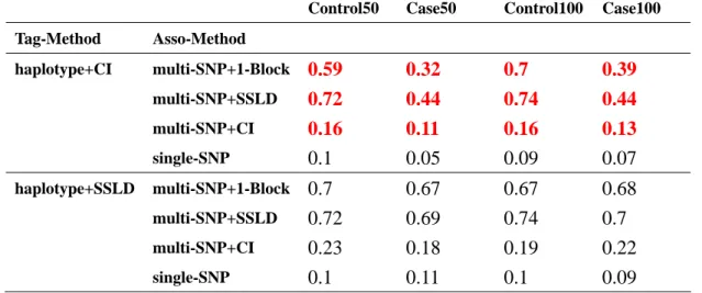
Then we would see different result in the second situation. When using the tag SNP method of haplotype+CI which were adverse result in sample of case-control. We could see that power in control was larger both in association sample size 500 or 200 at three multiple SNPs tests. The reason maybe tag SNPs selected by haplotype+CI got much information in control and almost in blocks not in SNPs outside blocks. These distinctions provided information for us to do decide later.
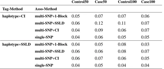
Despite using any association methods the sample size of 500 has large power the 200. Although it had a large power in sample size = 500, but it also cost much. So it was an important thing to find a balance between sample size and power. We would consider the variation of power of every method in the null region after be comparing the causal region. Because a good method was in addition to have higher power in the causal region and must have lower power in the null region. We could see multiple SNP test and single SNP test had the same level of lower power (Table 5, Table 6).
5.
Conclusion
Our goal for this study was to compare different tagging methods, haplotype blocking and association testing using different sample populations for tag SNP with respect to the power. We found that there were no significant differences in estimated power between the two tag SNP samples, 50 and 100. Large association samples would have to be recruited in order to offset the lower power. Then we would give some advise according to figure 6 to 11 in every situation and sample. We considered about number of tag SNPs and power’s level to choose a tagging method with an association test that cost less and powerful. When we had association sample = 500, four methods of tag NP match with the multi-SNP+1-Block had power about the same either in case or control, so we selected haplotype+1-Block because it had less number of tag SNPs. Although haplotype+CI had least number of tag SNPs in second situation, it’s power was lower than haplotype+1-Block about 10% in control and 40% in case. When matching with multi-SNP+SSLD we may select haplotype+1-Block in case and haplotype+CI of second situation in control. The powers in multi-SNP+CI and single-SNP were too small, so we would use the two methods to do association analysis. Then we consider about association sample = 200, we selected tag SNP method of SSLD match with multi-SNP+1-Block in second situation because it had the best power. Haplotype+CI in control and haplotype+1-Block in case were our choices when matching with multi-SNP+SSLD. These conclusions were applied only on rare allele, but other allele types may be not suitable. These conclusions will facilitate future decisions in this same population, and when analyze real data may make decisions refer to this.
Table 3. Association sample = 500cases-500controls in casual region Table 3.a. haplotype+CI and haplotype+SSLD using first situation
sample
Control50 Case50 Control100 Case100 Tag-Method Asso-Method tagger multi-SNP+1-Block 0.98 0.99 0.97 0.99 multi-SNP+SSLD 0.6 0.96 0.58 0.98 multi-SNP+CI 0.27 0.27 0.29 0.28 single-SNP 0.19 0.19 0.2 0.22 haplotype+CI multi-SNP+1-Block 0.99 0.99 0.99 0.99 multi-SNP+SSLD 0.98 0.98 0.98 0.98 multi-SNP+CI 0.29 0.27 0.29 0.23 single-SNP 0.2 0.19 0.22 0.21 haplotype+SSLD multi-SNP+1-Block 0.99 0.99 0.99 0.99 multi-SNP+SSLD 0.98 0.98 0.98 0.98 multi-SNP+CI 0.27 0.26 0.26 0.26 single-SNP 0.19 0.18 0.2 0.2 haplotype+1-Block multi-SNP+1-Block 0.95 0.97 0.97 0.99 multi-SNP+SSLD 0.57 0.89 0.7 0.95 multi-SNP+CI 0.26 0.21 0.23 0.26 single-SNP 0.21 0.2 0.18 0.21
Table 3.b. haplotype+CI and haplotype+SSLD using second situation.
Control50 Case50 Control100 Case100 Tag-Method Asso-Method haplotype+CI multi-SNP+1-Block 0.88 0.58 0.91 0.58 multi-SNP+SSLD 0.88 0.6 0.91 0.61 multi-SNP+CI 0.19 0.14 0.17 0.16 single-SNP 0.16 0.13 0.17 0.15 haplotype+SSLD multi-SNP+1-Block 0.99 0.99 0.99 0.99 multi-SNP+SSLD 0.98 0.98 0.98 0.97 multi-SNP+CI 0.26 0.25 0.26 0.26 single-SNP 0.2 0.21 0.21 0.2
Table 4. Association sample = 200cases-200controls in casual region Table 4.a. haplotype+CI and haplotype+SSLD used first situation
sample
Control50 Case50 Control100 Case100 Tag-Method Asso-Method tagger multi-SNP+1-Block 0.53 0.69 0.52 0.67 multi-SNP+SSLD 0.28 0.63 0.33 0.72 multi-SNP+CI 0.16 0.19 0.17 0.21 single-SNP 0.11 0.11 0.09 0.11 haplotype+CI multi-SNP+1-Block 0.68 0.69 0.68 0.68 multi-SNP+SSLD 0.73 0.71 0.75 0.73 multi-SNP+CI 0.21 0.18 0.21 0.22 single-SNP 0.09 0.1 0.1 0.11 haplotype+SSLD multi-SNP+1-Block 0.67 0.68 0.68 0.68 multi-SNP+SSLD 0.71 0.72 0.76 0.72 multi-SNP+CI 0.23 0.19 0.2 0.22 single-SNP 0.09 0.1 0.11 0.11 haplotype+1-Block multi-SNP+1-Block 0.48 0.63 0.56 0.64 multi-SNP+SSLD 0.41 0.67 0.42 0.71 multi-SNP+CI 0.11 0.14 0.15 0.17 single-SNP 0.1 0.09 0.11 0.11
Table 4.b. haplotype+CI and haplotype+SSLD using second situation.
Control50 Case50 Control100 Case100 Tag-Method Asso-Method haplotype+CI multi-SNP+1-Block 0.59 0.32 0.7 0.39 multi-SNP+SSLD 0.72 0.44 0.74 0.44 multi-SNP+CI 0.16 0.11 0.16 0.13 single-SNP 0.1 0.05 0.09 0.07 haplotype+SSLD multi-SNP+1-Block 0.7 0.67 0.67 0.68 multi-SNP+SSLD 0.72 0.69 0.74 0.7 multi-SNP+CI 0.23 0.18 0.19 0.22 single-SNP 0.1 0.11 0.1 0.09
Table 5. Association sample = 500cases-500controls in null region Table 5.a. haplotype+CI and haplotype+SSLD used first situation
sample
Control50 Case50 Control100 Case100 Tag-Method Asso-Method tagger multi-SNP+1-Block 0.05 0.04 0.05 0.05 multi-SNP+SSLD 0.05 0.04 0.07 0.05 multi-SNP+CI 0.04 0.08 0.06 0.06 single-SNP 0.05 0.06 0.06 0.07 haplotype+CI multi-SNP+1-Block 0.05 0.07 0.05 0.05 multi-SNP+SSLD 0.05 0.06 0.06 0.06 multi-SNP+CI 0.06 0.05 0.05 0.05 single-SNP 0.03 0.04 0.04 0.04 haplotype+SSLD multi-SNP+1-Block 0.05 0.06 0.05 0.05 multi-SNP+SSLD 0.06 0.05 0.06 0.06 multi-SNP+CI 0.05 0.07 0.05 0.05 single-SNP 0.04 0.05 0.04 0.04 haplotype+1-Block multi-SNP+1-Block 0.02 0.04 0.05 0.05 multi-SNP+SSLD 0.03 0.04 0.06 0.05 multi-SNP+CI 0.03 0.06 0.04 0.03 single-SNP 0.06 0.07 0.06 0.07
Table 5.b. haplotype+CI and haplotype+SSLD using second situation.
Control50 Case50 Control100 Case100 Tag-Method Asso-Method haplotype+CI multi-SNP+1-Block 0.05 0.07 0.07 0.06 multi-SNP+SSLD 0.06 0.12 0.11 0.07 multi-SNP+CI 0.04 0.09 0.06 0.07 single-SNP 0.04 0.06 0.05 0.05 haplotype+SSLD multi-SNP+1-Block 0.04 0.05 0.08 0.03 multi-SNP+SSLD 0.06 0.06 0.08 0.07 multi-SNP+CI 0.06 0.07 0.06 0.05 single-SNP 0.04 0.05 0.04 0.04
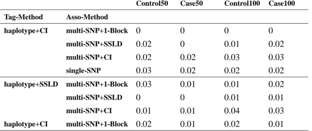
Table 6. Association sample = 500cases-500controls in null region Table 6.a. haplotype+CI and haplotype+SSLD used first situation
sample
Control50 Case50 Control100 Case100 Tag-Method Asso-Method tagger multi-SNP+1-Block 0 0 0.01 0 multi-SNP+SSLD 0.02 0.01 0.01 0 multi-SNP+CI 0.02 0.01 0.03 0.04 single-SNP 0.02 0.01 0.01 0.02 haplotype+CI multi-SNP+1-Block 0.02 0.02 0.01 0.01 multi-SNP+SSLD 0.01 0 0.01 0.02 multi-SNP+CI 0.01 0 0.03 0.03 single-SNP 0.02 0.01 0.01 0.01 haplotype+SSLD multi-SNP+1-Block 0.01 0.02 0 0 multi-SNP+SSLD 0.01 0 0.01 0.01 multi-SNP+CI 0.02 0.01 0.04 0.03 single-SNP 0.02 0.01 0.01 0.01 haplotype+1-Block multi-SNP+1-Block 0.01 0.01 0.01 0.01 multi-SNP+SSLD 0 0.02 0.01 0.02 multi-SNP+CI 0.02 0.04 0.03 0.03 single-SNP 0.02 0.02 0.02 0.02
Table 6.b. haplotype+CI and haplotype+SSLD using second situation.
Control50 Case50 Control100 Case100 Tag-Method Asso-Method haplotype+CI multi-SNP+1-Block 0 0 0 0 multi-SNP+SSLD 0.02 0 0.01 0.02 multi-SNP+CI 0.02 0.02 0.03 0.03 single-SNP 0.03 0.02 0.02 0.02 haplotype+SSLD multi-SNP+1-Block 0.03 0.01 0.01 0.02 multi-SNP+SSLD 0 0 0.01 0.01 multi-SNP+CI 0.01 0.01 0.04 0.03 haplotype+CI multi-SNP+1-Block 0.02 0.01 0.02 0.01
Tagger 0 0.2 0.4 0.6 0.8 1
Multi-SNP+1-Block Multi-SNP+SSLD Multi-SNP+CI Single-SNP
po
w
er
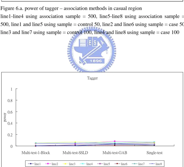
line1 line2 line3 line4 line5 line6 line7 line8 Figure 6.a. power of tagger – association methods in casual region
line1-line4 using association sample = 500, line5-line8 using association sample = 500, line1 and line5 using sample = control 50, line2 and line6 using sample = case 50, line3 and line7 using sample = control 100, line4 and line8 using sample = case 100
Tagger 0 0.2 0.4 0.6 0.8 1
Multi-test-1-Block Multi-test-SSLD Multi-test-GAB Single-test
pow
er
line1 line2 line3 line4 line5 line6 line7 line8
haplotype+CI 0 0.2 0.4 0.6 0.8 1 1.2
Multi-SNP+1-Block Multi-SNP+SSLD Multi-SNP+CI Single-SNP
pow
er
line1 line2 line3 line4 line5 line6 line7 line8
Figure 7.a. power of haplotype+CI – association methods in casual region in first situation haplotype+CI 0 0.2 0.4 0.6 0.8 1
Multi-SNP+1-Block Multi-SNP+SSLD Multi-SNP+CI Single-SNP
po
w
er
line1 line2 line3 line4 line5 line6 line7 line8
Figure 7.b. power of haplotype+CI – association methods in null region in first situation
haplotype+SSLD 0 0.2 0.4 0.6 0.8 1 1.2
Multi-SNP+1-Block Multi-SNP+SSLD Multi-SNP+CI Single-SNP
pow
er
line1 line2 line3 line4 line5 line6 line7 line8
Figure 8.a. power of haplotype+SSLD – association methods in casual region in first situation haplotype+SSLD 0 0.2 0.4 0.6 0.8 1
Multi-SNP+1-Block Multi-SNP+SSLD Multi-SNP+CI Single-SNP
pow
er
line1 line2 line3 line4 line5 line6 line7 line8
Figure 8.b. power of haplotype+SSLD – association methods in null region in first stuation
haplotype+1-Block 0 0.2 0.4 0.6 0.8 1
Multi-SNP+1-Block Multi-SNP+SSLD Multi-SNP+CI Single-SNP
pow
er
line1 line2 line3 line4 line5 line6 line7 line8
Figure 9.a. power of haplotype+1-Block – association methods in casual region in first situation haplotype+1-Block 0 0.2 0.4 0.6 0.8 1
Multi-SNP+1-Block Multi-SNP+SSLD Multi-SNP+CI Single-SNP
po
w
er
line1 line2 line3 line4 line5 line6 line7 line8
Figure 9.b. power of haplotype+1-Block – association methods in null region in first situation
haplotype+CI 0 0.2 0.4 0.6 0.8 1
Multi-SNP+1-Block Multi-SNP+SSLD Multi-SNP+CI Single-SNP
po
w
er
line1 line2 line3 line4 line5 line6 line7 line8
Figure 10.a. power of haplotype+CI – association methods in casual region in second situation haplotype+CI 0 0.2 0.4 0.6 0.8 1
Multi-SNP+1-Block Multi-SNP+SSLD Multi-SNP+CI Single-SNP
po
wer
line1 line2 line3 line4 line5 line6 line7 line8
Figure 10.b. power of haplotype+CI – association methods in null region in second situation
haplotype+SSLD 0 0.2 0.4 0.6 0.8 1
Multi-SNP+1-Block Multi-SNP+SSLD Multi-SNP+CI Single-SNP
po
w
er
line1 line2 line3 line4 line5 line6 line7 line8
Figure 11.a. power of haplotype+SSLD – association methods in casual region in second situation haplotype+SSLD 0 0.2 0.4 0.6 0.8 1
Multi-SNP+1-Block Multi-SNP+SSLD Multi-SNP+CI Single-SNP
po
we
r
line1 line2 line3 line4 line5 line6 line7 line8
Figure 11.b. power of haplotype+SSLD – association methods in null region in second situation
References
1. Wang DG, Fan JB, Siao CJ, Berno A, Young P, Sapolsky R, Ghandour G, et al Large Scale identification, mapping and genotyping of single-nucleotide
polymorphisms in the human genome. 1998; Science 280:1077–1082.
2. Zhang K, Calabrese P, Nordborg M, Sun F. Haplotype Block Structure and Its Applications to Association Studies: Power and Study Designs. Am J Hum Genet. 2002; Nov 18;71(6).
3. Balding DJ, A tutorial on statistical methods for population association studies. 2006;Nat Rev Genet. 7:781-791
4. De Bakker PI, Yelensky R, Pe'er I, Gabriel SB, Daly MJ, Altshuler D. Efficiency and power in genetic association studies. 2005; Nat Genet 37:1217-23.
5. Stram DO. Tag SNP selection for association studies. 2004; Genetic Epidemiology 27: 365–374.
6. Gabriel SB, Schaffner SF, Nguyen H, Moore JM, Roy J, Blumenstiel B, Higgins J,DeFelice M, Lochner A, Faggart M, Liu-Cordero SN, Rotimi C, Adeyemo A, Cooper R,Ward R, Lander ES, Daly MJ, Altshuler D. The structure of haplotype blocks in the human genome. 2002; Science 296:2225–2229.
7. Barrett JC, Fry B, Maller J, Daly MJ. Haploview: analysis and visualization of LD and haplotype maps.2005; Bioinformatics 21: 263–265.
8. Robbins, R.B. Some applications of mathematics to breeding problems III. 1918; Genetics 3: 375-389
9. Lewontin, R.C. and K. Kojima . The evolutionary dynamics of complex polymorphisms. 1960; Evolution 14: 458-472
10. Lewontin, R.C. The interaction of selection and linkage. I. General considerations: heterotic models.1964; Genetics, 49, 49-67.
11. Wang, N., Akey, J.M., Zhang, K., Chakraborty, K., and Jin, L. Distribution of recombination crossovers and the origin of haplotype blocks: The interplay of population history.2002.
12. Patil, N., Berno, A.J., Hinds, D.A., Barrett, W.A., Doshi, J.M., Hacker, C.R., Kautzer,C.R., Lee, D.H., Marjoribanks, C., McDonough, D.P., et al. Blocks of limited haplotype diversity revealed by high-resolution scanning of human chromosome 21. 2001; Science 294: 1719–1723.
13. Zhang, K., Deng, M., Chen, T., Waterman, M.S., and Sun, F. A dynamic programming algorithm for haplotype block partitioning. Proc. Natl. Acad. 2002b; Science. 99: 7335–7339.
15. Clayton D.2005. SNPHAP: a program for estimating frequencies of large haplotypes of SNPs (Version1.3)
[http://www.gene.cimr.cam.ac.uk/clayton/software/]
14. Davs J. Balding. A tutorial on statistical methods for population association studies. 2006; Genetic
16. P.I.W. de Bakker, R. Yelensky, I. Pe'er, S.B. Gabriel, M.J. Daly, D. Altshuler Efficiency and power in genetic association studies. 2005; Nature Genetics. 37: 1217-1223
17. Chi PB, Duggal P, Kao WHL, Mathias RA, GrantAV, Stockton ML, Garcia JGN, Ingersoll RG, Scott AF, Beaty TH, Barnes KC, Fallin MD. Comparison of SNP tagging methods using empirical data: association study of 713 SNPs on
chromosome 12q14.3-12q24.21 for asthma and total serum IgE in an African Caribbean population. 2006; Genetic Epidemiology; 30:609 - 619
18. Stram DO, Haiman CA, Hirschhorn JN, Altshuler D, Kolonel LN, Henderson BE,Pike MC. Choosing haplotype-tagging SNPs based on unphased genotype
multiethnic cohort study. 2002; Hum Hered. 55:27-36
19. Julian Forton, Dominic Kwiatkowski, Kirk Rockett, Gaia Luoni, Martin Kimber, and Jeremy Hull.Accuracy of Haplotype Reconstruction from Haplotype-Tagging Single-Nucleotide Polymorphisms. 2005.
20. Kelly M Bukett, Mercedeh Ghadessi, Brad McNeney, Jinko Graham and Denise Daley. 2004. A comparison of five methods for selecting tagging
single-nucleotide polymorphisms.2005; BMC Genetics, 6:S71
21. Kui Zhang, Zhaohui S. Qin, Jun S. Liu, Ting Chen, Michael S. Waterman and Fengzhu Sun.2004.Haplotype Block Partitioning and Tag SNP Selection Using Genotype Data and Their Applications to Association Studies. 2004; Genome Res 14: 908-916.