低功率系統之設計及自動化-子計畫一：適用於行動裝置之前瞻功率認知系統設計(III)

行政院國家科學委員會專題研究計畫 成果報告

子計畫一：適用於行動裝置之前瞻功率認知系統設計(3/3)

中 華 民 國 95 年 10 月 31 日

中文摘要

Wireless sensor network是近年來一個十分熱門的研究領域。在sensor network 當 中 ， 通 常 會 有 許 多 節 點 共 用 同 一 個 channel ， 這 會 造 成 channel sharing problem，例如：增加route discovery的複雜度、降低network performance以 及因為訊號的干擾而必須重傳封包，這會使得energy consumption增加。為了解 決上述的問題，有許多網路拓樸控制的演算法被提出來。其中，最廣為使用的就 是backbone機制。到目前為止，大多數的backbone演算法都著重在從整個網路當 中挑選出適當的節點作為coordinators以減少backbone size，然而過少的 coordinators用來轉送封包將造成效能不佳等負面影響。所以許多啟發式的演算 法被提出來，但是這些演算法並不能夠有效率地將多餘的節點除去，以及在稀疏 的網路狀態下，網路傳輸效能會大幅度降低。本計畫第一部分的目標是提供一個 新 穎 的 backbone 演 算 法 稱 為 SmartBone ， 我 們 提 出 先 使 用 Flow-Bottleneck preprocessing 來 找 出 所 有 的 critical nodes ， 這 些 節 點 能 夠 增 加 connectivity，以及提出Dynamic Density Cutback來將多餘的節點去除掉。 SmartBone同時考慮了網路效能以及能源的消耗。採用SmartBone能夠降低一半的 backbone size，並且能夠將能源的節省率從採用傳統方法的25%提升到40%，這 將節省了大量的能源消耗。另外，在sensor network中的一些節點因為電源耗盡 或故障，使得網路的拓樸變得比較稀疏，在這樣惡劣的網路環境下，我們的 SmartBone能夠將packet delivery ratio從採用傳統方法的40%提升到90%。 sensor network 存 在 另 外 一 個 潛 在 的 問 題 ， 就 是 如 何 有 效 率 的 把 封 包 從 single-source傳送至multi-sinks。也就是從一個sensor node把資料收集起 來，然後傳給對此資料有興趣的多個clients。要處理這種情況的困難之處在於 尋找minimum-cost transmission paths，已經有很多routing algorithm被提出 來解決這個問題，但是現存的演算法大部分著重於減少能量的消耗。所以當只考 慮能量因素時，顯而易見的是會產生很大的延遲現象。本計畫的第二部分提出一 個新穎的multi-path routing algorithm 使用在無線感測器網路環境下。這裡 提供了稱為Hop-Count based Routing (HCR) algorithm，此方法同時考慮了能 量消耗與傳送的延遲。我們採用了hop count vector (HCV) 來幫助routing decision 。 另 外 ， 加 上 pruning vector (PV) 可 以 更 加 提 昇 routing performance。我們提出的演算法也提供了maintenance mechanism以處理failed nodes帶來的影響。一個node的錯誤就會使得HCV不正確。所以需要一個有效率的 更 正 演 算 法 。 我 們 提 出 Aid-TREE (A-TREE) 的 演 算 法 可 以 很 容 易 地 採 用 restricted flooding，這種更正機制比full-scale flooding來得有效率。最後， 我 們 研 究 了 failed nodes 對 整 個 網 路 拓 樸 的 影 響 ， 並 且 提 出 一 個 叫 做 lazy-grouping的演算法，來增進HCR的穩定度。

關鍵字：網路骨幹、拓樸控制、分散式深度優先演算法、多重路徑路由、路徑合 併、無線感測器網路。

Abstract

Wireless sensor network is a rapidly growing discipline with new technologies emerging, and new applications under development. Wireless sensor nodes deposited in various places can measure light, humidity, temperature, etc. and can therefore be used in applications such as security surveillance, environmental monitoring and wildlife watching. A communication channel is generally shared among many sensor nodes in wireless sensor networks. Such sharing reduces the network performance due to aggravated radio interference. At same time it raises energy consumption since packet retransmission is needed when interference occurs. Moreover, the energy consumption could be skyrocket if we don’t limit number of active sensor nodes for the data relays. Topology control can be utilized to address the above problems. Topology control will remove unnecessary transmission links by shutting down some of redundant nodes. Nevertheless topology control will still guarantee network connectivity in order to deliver data efficiently in a wireless sensor network. This report proposes two topology control schemes, namely SmartBone and HCR (Hop Count based Routing) separately, in wireless sensor networks. The first scheme in the report, SmartBone, proposes a novel mechanism to construct a backbone. Some nodes are chosen as coordinators (i.e. backbone nodes) in the backbone construction process. All nodes then can directly or indirectly communicate with other nodes via these coordinators. The coordinators form the backbone, and the non-selected nodes can perform sleeping schedule or turn off the radio to save the energy consumption. Another potential application model for a sensor network is transmitting packets efficiently from Single-Source to Multi-Sinks. It is to gather data from a single sensor node and deliver it to multiple clients who are interested in the data. This in wireless sensor network model is called Single-Source to Multi-Sinks (SSMS). The difficulty of handling the model is in how to arrange the minimum-cost transmission path. The second proposed scheme in the report, HCR, simultaneously addresses energy-cost and end-to-end delay to solve the above problem.

Keywords: backbone, topology control, distributed DFS, flow-bottleneck preprocessing, critical nodes, density cutback, multi-path routing, path aggregation, prune vector, set cover, grouping, robustness, wireless sensor networks

Table of Content

Chapter 2: SmartBone: An Energy-Efficient Smart Backbone Construction in Wireless Sensor Networks ...1

2.1 Introduction...1

2.2 SmartBone Design ...4

2.2.1 Neighborhood Information Collection...5

2.2.2 Flow-Bottleneck Preprocessing ...5

2.2.3 BackBone Selecting Procedure...9

2.3 Performance Simulation and Analysis ...15

2.3.1 Performance metrics ...15

2.3.2 Simulation Environment ...15

2.3.3 Simulation Results ...16

2.3.4 Sensitivity of thresholds...19

Chapter 3: Minimum-Delay Energy-Efficient Source to Multisink Routing in Wireless Sensor Networks ...21

3.1 Introduction...21

3.2 HCR Algorithm...22

3.2.1 Hop Count Vector ...22

3.2.2 Next Hop Selection...26

3.2.3 Extended Set Cover with Load-Balance ...27

3.2.4 Prune Vector...29

3.3 HCR Maintenance Scheme ...31

3.3.1 Flooding Scope ...31

3.3.2 Aid-TREE ...32

3.4 Robustness Improvement...34

3.5 Simulation Results and Performance Analysis ...37

3.5.1 Performance metrics ...37

3.5.2 Simulation Scenarios ...38

3.5.3 Performance Result and Analysis ...40

Chapter 4: Conclusions ...51

List of Figures

Fig. 1. DDFS procedure...8

Fig. 2. Example of SmartBone construction...14

Fig. 3. Average number of coordinators elected by the protocols during the simulation duration ...16

Fig. 4. Average number of coordinators elected by the protocols tests under different network density...17

Fig. 5. Packet delivery ratio tests under different network density...17

Fig. 6. Energy saving ratio tests under different network density ...18

Fig. 7. Example of SSMS model ...23

Fig. 8. Transmission path of BF method...24

Fig. 9. Transmission path of Power-Optimization method ...24

Fig. 10. Transmission path of the best solution ...25

Fig. 11. Example of HCV1 ...25

Fig. 12. Example of HCV2 ...26

Fig. 13. Example of next hop selection...27

Fig. 14. Example of Extended Set Cover...28

Fig. 15. Example that after N3 is selected ...29

Fig. 16. Final result of the next hop selecting procedure...29

Fig. 17. The next hop selection without PV...30

Fig. 18. Example of PV...31

Fig. 19. Operation of finding an A-TREE...33

Fig. 20. The first phase of finding an A-TREE...33

Fig. 21. The second phase of finding an A-TREE ...34

Fig. 22. A final A-TREE ...34

Fig. 23. Example of Lazy Grouping ...35

Fig. 24. Network topology without LG ...36

Fig. 25. Network topology with LG...36

Fig. 26. Full-Corner 4/8/16 topology...39

Fig. 27. Full-Corner 4: Node density VS. number of transmission ...40

Fig. 28. Full-Corner 8: Node density VS. number of transmission ...41

Fig. 29. Full-Corner 16: Node density VS. number of transmission ...41

Fig. 30. Block 4: Node density VS. number of transmission ...42

Fig. 31. Corner 4: Node density VS. number of transmission...42

Fig. 32. Line 4: Node density VS. number of transmission...43

Fig. 33. Line 8: Node density VS. number of transmission...43

Fig. 34. Line 16: Node density VS. number of transmission...44

Fig. 36. Cycle 8: Node density VS. number of transmission...45

Fig. 37. Cycle 16: Node density VS. number of transmission...45

Fig. 38. Cycle 32: Node density VS. number of transmission...46

Fig. 39. Energy cost using LG-HCR...46

Fig. 40. Robustness of HCR and LG-HCR...47

Fig. 41. Flooding scope of HCR and LG-HCR ...48

Fig. 42. Improvement in robustness using LG-HCR over HCR...48

Fig. 43. Node density VS. transmission delay ...49

Fig. 44. Comprehensive comparison between HCR and LG-HCR ...49

List of Tables

Table I. FLOW_TH used during simulation ...8 Table II. CUT_TH and boundary of local node density used during simulation...12

Chapter 1: Introduction

Wireless sensor network is a rapidly growing discipline with new technologies emerging, and new applications under development. Wireless sensor nodes deposited in various places enable the measurement of light, temperature, humility, etc. In addition to providing light and temperature measurements, wireless sensor nodes have applications such as security surveillance, environmental monitoring, and wildlife watching. The nodes in a wireless network generally to communicate with each other along the same wireless channel. Unfortunately, sharing among wireless channels decreases network performance due to radio interference, and also raises energy consumption due to packet retransmission when interference occurs. Many topology control algorithms have been proposed to solve these problems. One widely used strategy is the backbone method. Backbone algorithms aim to reduce the backbone size. However, poor performance may be explored if only few backbone nodes are selected. Therefore, several heuristic algorithms such as SBC have been proposed. However, these algorithms cannot efficiently eliminate redundant nodes, and dramatically decrease performance especially in sparse networks. The first scheme in the report proposes a novel backbone algorithm called SmartBone to choose proper backbone nodes from a network. SmartBone includes two major mechanisms. Flow-Bottleneck preprocessing is adopted to find critical nodes, which act as backbone nodes to improve connectivity. Dynamic Density Cutback is adopted to reduce the number of redundant nodes depending on area node density of network. SmartBone simultaneously considers the balance of network performance and energy savings. Significantly, the proposed algorithm has a 50% smaller backbone size than SBC, and improves the energy saving ratio from 25% using SBC to 40% using SmartBone. Moreover, SmartBone improves the packet delivery ratio from 40% to 90% even in the sparse networks.

Another important problem in a sensor network is how to transmit packets efficiently from Single-Source to Multi-Sinks. It is to gather data from a single sensor node and deliver it to multiple clients who are interested in the data. The difficulty of handling such a scenario is in finding the minimum-cost multiple transmission paths. Many routing algorithms have been proposed to solve this problem. Most current algorithms address the reduction of power consumption. Therefore, a large delay can be explored if only the energy factor is considered. The second scheme in the report proposes a novel multi-path routing algorithm in wireless sensor networks. A routing algorithm called Hop-Count based Routing (HCR) algorithm, which considers energy cost and transmission delay simultaneously, is provided. A hop count vector (HCV) is

introduced to support routing decision. Moreover, an additional pruning vector (PV) can further enhance routing performance. The proposed algorithm also provides a maintenance mechanism to handle the consequence of faulty nodes. A failure of a node leads to an inaccurate HCV. Therefore, an efficient correction algorithm is necessary. An Aid-TREE (A-TREE) is applied to facilitate restricted flooding. This correction mechanism is more efficient than full-scale flooding for correcting the limited inaccurate HCVs. Finally, the impact of failed nodes is studied, and an algorithm, called Lazy-Grouping, is proposed to enhance the robustness of HCR.

Chapter 2: SmartBone: An Energy-Efficient Smart

Backbone Construction in Wireless Sensor Networks

2.1 Introduction

Wireless sensor network is a rapidly growing discipline with new technologies emerging, and new applications under development. Wireless sensor nodes deposited in various places can measure light, humidity, temperature, etc. and can therefore be used in applications such as security surveillance, environmental monitoring and wildlife watching [20], [28], [34], and [27]. A communication channel is generally shared among many sensor nodes in wireless sensor networks. Such sharing reduces the network performance due to aggravated radio interference. At same time it raises energy consumption since packet retransmission is needed when interference occurs. Moreover, the energy consumption could be skyrocket if we don’t limit number of active sensor nodes for the data relays. Topology control can be utilized to address the above problems. Topology control will remove unnecessary transmission links by shutting down some of redundant nodes. Nevertheless topology control will still guarantee network connectivity in order to deliver data efficiently in a wireless sensor network.

The following criteria are typically applied to evaluate the performance of the topology control [1]: connectivity, energy-efficiency, throughput and robustness. Energy consumption is the most significant issue in wireless sensor networks, since most sensors are powered by batteries. Power supply issue is a severe limitation in sensor application, since sensors must operate for a long time (i.e., for many years) and can not be recharged while they are operating.

Topology control for energy-saving can be accomplished in two ways. The first method involves adjusting the radio power to maintain the proper number of neighbors [21][22]. The second method involves turning off the radio power or performing some sleeping schedules for some redundant nodes to reduce the unnecessary energy consumption [6]. At some time maintain a sufficient number of active nodes to perform data forwarding.

An effective topology control can enhance network performance by reducing interference and increase network life time by saving energy. Adjusting the transmission range and reducing the number of redundant nodes are both methods for achieving this goal. The first method saves less energy than the second, because

adjusting the transmission range does not turn the radio off. Turning off the radio in the redundant nodes is a rational idea, since nodes incur the same energy costs both in active communication and in the idle state. Estrin et. Al. [2] indicates that the energy consumption in the transmission and idle states are similar. However, the energy consumption of a sleeping node is 1000 times less than that of an active node [3]. This large ratio can be exploited to economize on energy. Several methods exist to reduce the number of redundant nodes such as a backbone-based [6][7][10][4] or cluster-based algorithms [12][13].

In this section, we propose a novel mechanism called SmartBone to construct a backbone. Some nodes are chosen as coordinators (i.e. backbone nodes) in the backbone construction process. All nodes then can directly or indirectly communicate with other nodes via these coordinators. The coordinators form the backbone, and the non-selected nodes can perform sleeping schedule or turn off the radio to save the energy consumption.

The backbone-based algorithms can be classified based on size of constructed backbone. According to backbone size, the schemes can be divided into non-constant [6][14][15][16][17] and constant ratio schemes [4][9][18][19]. The backbone size needs to be reduced to maximize the energy saving. Therefore, minimizing the backbone is normally the best policy. However, the problem of constructing minimum backbone is equivalent to the problem of finding the minimum connected dominating set (MCDS) in the graph theory. Unfortunately it is a classic NP-hard optimization problem. Constant ratio schemes ensure that the constructed backbone size should be bounded by a certain ratio against size of MCDS. Non-constant schemes would not have above property.

Although minimizing the backbone size can save a large amount of energy, it also causes poor network performance due to resource competition and network congestion. Algorithms that simultaneously optimize the energy consumption and network performance have proved impossible to obtain [5]. However, a trade-off does exist between the minimum energy cost and minimum congestion. In SmartBone, we attempt to balance of the sustainability of energy cost and network performance.

SBC [6] is a heuristic-based non-constant backbone construction method. It constructs a backbone by determining which node should be selected as coordinator of backbone. SBC divides all nodes into two groups and judges within the same group whether a node are a redundant node. Redundant nodes are those that are close to each

other in the same group, and will not be chosen as coordinators. A drawback of the SBC algorithm is its lack of a good overlap detection method. SBC cannot efficiently delete nodes that are very close to each other locally, because it considers the global redundancy threshold which determined the ratio of common neighbors. However, SmartBone adopts a Dynamic Density Cutback (DDC) mechanism to reduce the number of redundant nodes according to the dynamic thresholds which is determined by node density of network topology. In SmartBone, node degree is used as the indicator of node density.

Another drawback of SBC is its partition method. SBC partitions nodes into two groups, and picks up some nodes individually from both groups to form the backbone. Therefore, the nodes chosen from one group may be too close the nodes chosen from the other group. The third drawback is also a problem exists in most of backbone methods. Currently most of backbone methods work inefficiently in sparse topology due to the lack of critical nodes awareness mechanism. That is, when choosing nodes as the backbone nodes, the methods do not consider which nodes have critical property such as cut points of the network. Therefore, more coordinators are needed to ensure acceptable network performance such as packet delivery ratio.

However, SmartBone adopts an efficient mechanism to choose coordinators. We observe that choosing articulation points (cut points) as backbone nodes is just a rudimentary requirement. We grantee that the nodes (containing cut points) which on the critical communication paths would be selected as backbone nodes. Therefore, packet deliver is not restricted to only few transmission paths. Choosing necessary critical nodes for the backbone is useful, particularly in a sparse topology which has few communication links.

SmartBone provides a general backbone solution, and can efficiently control the backbone nodes selection. The DDC feature of SmartBone can delete many redundant nodes in a dense topology without affecting network performance.

It is noteworthy that backbone algorithm generally starts by electing several backbone seeds in the topology and then completes backbone construction by making a sweep of the network spreading outwards from the backbone seeds. Backbone seeds choose appropriate neighbor nodes as coordinators to connect to remote nodes. Therefore, it is discussible with the selection of backbone seeds. Ideal backbone seeds should have high priority such as high residual energy or large coverage. SBC chooses backbone seeds from an area of high node density so that more nodes can be

covered quickly. SmartBone extends the consideration advisedly. Backbone seeds are chosen based on the 2-hop neighbors’ information. After collecting neighborhood information, SmartBone performs FlowBP to choose critical nodes. Therefore, these critical nodes are especially chosen to act as the backbone seeds. Subsequently, SmartBone starts from these seeds. We would present the significance of the critical nodes in later section.

The rest of this section is organized as follows. Section II presents a SmartBone example, and elaborates on the design of the SmartBone protocol, problems encountered in the design, and the novel way in which these problems were solved. Next, Section III describes our simulation setup and reports the simulation results in detail. Conclusions are finally drawn in Section IV.

2.2 SmartBone Design

The proposed algorithm assumes that each device has the same transmission range. Hence, the connection between any pair of nodes is bidirectional. Each node needs to be prioritized to select appropriate nodes from entire network to build up the backbone and to maintain an appropriate backbone size. The priority of nodes can be calculated in various ways. Bao and Garcia-Luna-Aceves [8] proposed some criteria for setting the priorities of nodes such as residual energy. In order to extend network life time, we do not hope only few nodes exhaust their power as coordinators. Therefore, the energy threshold is set. When the node’s energy is below the threshold, it can still perform the regular routine, but is not suitable as coordinator to relay packets.

SmartBone considers two factors, namely the residual energy and the coverage. The priority is a linear combination of these two factors. The proportion of the two factors is adjusted by network designer according to network characteristics. The general recommended criteria are as follows. When residual energy accounts for a large proportion, it generally balances the power consumption of nodes in the network. Since every round picks out coordinator, the nodes with the superior residual energy are chosen as backbone nodes. These nodes consume energy by relaying packets, and then have lower priority than their neighbor nodes in the next round. When coverage accounts for a large proportion, it generally reduces the backbone size. Since the nodes chosen from candidates in each round are those with the largest coverage, it causes many redundant nodes to be deleted. Then, after picking out nodes with largest coverage for backbone each round, fewer nodes are available to be selected as

coordinators. SmartBone adopts a linear combination of these two factors. Many other approaches, including the exponential form, were tried in SmartBone. Finally, the simplest approach has been found to work best.

SmartBone is partitioned into three phases. The first phase is the Neighborhood information collection, in which the 2-hop neighbor information of each node is gathered to support necessary operations for later steps. The second phase is the Flow-Bottleneck Preprocessing (FlowBP), in which the whole network topology is checked, and critical nodes are collected based on the flow threshold. These critical nodes are act as backbone seeds and backbone selection algorithm starts from these seeds. The third phase is the Backbone selecting procedure, which is further subdivided into Backbone node selection and Dynamic Density Cutback (DDC). Backbone node selection selects coordinators according to the priority determined by linear combination of residual energy and coverage. Finally, the DDC procedure is performed to remove redundant nodes based on a cutback threshold.

2.2.1 Neighborhood Information Collection

To ensure that the SmartBone can make the appropriate decision, the necessary 2-hop neighbors’ information needs to be obtained. This information includes neighbors’ priority, and whether neighbors are the backbone nodes. Each node collects 2-hop neighbors’ information by exchange 1-hop neighbors’ information. Several approaches exist to obtain 1-hop neighbor information. For example, each node broadcasts hello packet periodically, or neighbors’ information piggyback with the data packets. SmartBone adopts the former approach.

2.2.2 Flow-Bottleneck Preprocessing

Backbone seeds are chosen based on the 2-hop neighbors’ information. After collecting neighbor information, SmartBone performs FlowBP to choose critical nodes. It is noticeable that those critical nodes contain articulation points. Therefore, these critical nodes are especially chosen to act as the backbone seeds. The connectivity can be improved in several ways, such as adding nodes [23], deploying MicroRouters [24], and using movable mobile routers [25]. SmartBone adopts Flow-Bottleneck to ensure critical nodes to be selected as coordinators. Critical nodes are nodes which on the critical communication paths in the network, and critical nodes contain cut points deservedly.

Preprocessing which other methods (ex: SBC) does not cost. However, FlowBP only runs once after network deployment in a topology. Hence, the overhead of FlowBP is negligible regarding the whole communication lifetime. In addition, the dense topology would become a sparse topology as time goes by, since it always exist nodes which consume a significant amount of energy in the network. The FlowBP would have to run again to accommodate to the new topology in such circumstances.

As noted previously, FlowBP allows SmartBone to maintain necessary connectivity, particularly in a sparse topology. FlowBP can detect the fragile part of many possible link paths, and make sure those links are includes in the backbone. The following is the detail procedure.

1) Distributed Depth First Search (DDFS)

The purpose of Distribute Depth First Search (DDFS) is to find the number of different possible paths to reach each node. DDFS extended the Depth First Search (DFS) algorithm to find N spanning trees in the network topology, where N is number of nodes. We emulate a situation that each node of network sends a packet to entire network through a spanning tree. Each node records its parents for each spanning trees. Number of different parents for each node gives us how many possible links to reach this node. The node with small number of different parents indicates that most of packets reach this node by few bridges. Therefore, it’s important to identify two end nodes of the bridge as critical nodes. FlowBP has two main steps. The first step is the Distributed Depth First Search (DDFS) processing, and the second is Flow-Bottleneck checking. In the first step, the DDFS algorithm is performed on each node. The following is the data structure used, and the detailed DDFS procedure as illustrated in Fig. 1.

% The following is pseudo-code for DDFS

% procedure. We emulate the operation of stack % to perform distributed DFS algorithm. The data % structure of DDFS is defined as follows:

%

% PRED : the parent node ID

% CHILD : the child node ID

% VISITED : has been visited or not

% DISCOVER : the order of visit

% NOWTIME : virtual visited order

% In the beginning, the DFS_ROOT performs

% DFS_ROOT_TASK() to launch the DFS_SPANNING() % procedure. If a node is DFS_ROOT, it sets PRED % as itself and notifies its 1-hop

% neighbors with 'DFS_VISITED' message.

PROCEDURE DFS_ROOT_TASK(): PRED := DFS_ROOT VISITED := 1 DISCOVER := 1 NOWTIME := 2 broadcast ( "DFS_VISITED" )

performs DFS_SPANNING() PROCEDURE ENDPROCEDURE

% PROCEDURE DFS_SPANNING()

% When node-v performs DFS_SPANNING(), it checks % whether it can choose a non-visited node-w % from NEIGHBOR_LIST. If exists such node-w then % node-v notifies node-w with 'DFS_BEGIN'

% message. It is equivalent to the 'PUSH'

% operation on the stack% Otherwise, it equals % to the 'POP' operation and node-v notifies % its parent with 'DFS_BACK' message.

PROCEDURE DFS_SPANNING():

IF ( select non-visited w from NEIGHBOR_LIST ) {

add w to CHILD

% 'PUSH' operation

send ( "DFS_BEGIN", NOWTIME) to w }

ELSE {

send ( "DFS_BACK" ) to PRED }

ENDPROCEDURE

% If a node receives 'DFS_VISITED' message from % node-p, it removes node-p from its own

% NEIGHBOR_LIST.

PROCEDURE DFS_VISITED():

removes p from NEIGHBOR_LIST ENDPROCEDURE

% If a node receives 'DFS_BEGIN' from node-v, % it's its turn to perform DFS_SPANNING() % procedure. PROCEDURE DFS_BEGIN(): PRED := v VISITED := 1 DISCOVER := NOWTIME + 1 broadcast ( "DFS_VISITED" )

performs DFS_SPANNING() PROCEDURE ENDPROCEDURE

% If node-p receives 'DFS_BACK' which send to % itself from node-v, it means that node-v

% finishes the exploration of spanning tree which rooted from % itself. Hence, node-p proceeds to DFS_SPANNING

% to explore the remainder network topology.

PROCEDURE DFS_BACK():

performs DFS_SPANNING() PROCEDURE ENDPROCEDURE

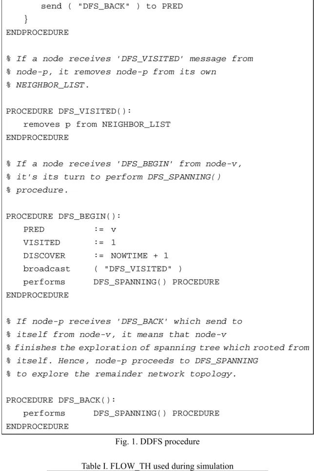
Fig. 1. DDFS procedure

Table I. FLOW_TH used during simulation Average Network Density 20 15 10 8

The conventional DFS algorithm often utilizes recursion, and it generally manipulates the stack to simulate recursion. DDFS simulates stack operation by sending control messages between nodes. For example, a PUSH stack operation corresponds to selecting a node from the NEIGHBOR_LIST and marking it as visited. At this moment, the visited nodes send DFS_BEGIN messages to non-visited nodes, as shown in ‘IF’ segment of Fig. 1. Conversely, a POP stack operation indicates that non-visited nodes can no longer be found in the NEIGHBOR_LIST, that is, the NEIGHBOR_LIST is null. The node with a null NEIGHBOR_LIST sends DFS_BACK message to DFS_PRED, as shown in ‘ELSE’ segment of Fig. 1. DDFS can simulate stack operation entirety, so the DFS algorithm can be applied on each node in a distributed fashion.

2) FlowBP Checking

The DDFS procedure is finished N times, where N represents the number of network nodes so that the information needed by FlowBP can be obtained. All nodes are then checked to determine which critical nodes are. The DFS_PRED of each node is checked after repeating DDFS N times. DFS_PRED records the parent IDs of each node. If the number of different parents of one node as recorded in DFS_PRED is below a threshold (FLOW_TH), then the node and corresponding parent node are selected as critical nodes. Since the FlowBP can identify these critical nodes, particularly in sparse topology, sufficient nodes are in the awaken state can be found to act as coordinators and relay packets. However, a node with large different parents under DDFS indicates that it can be reached through many possible paths. Therefore, if some of the paths are failed or obstructed, then the packets can still reach the same destination node through other paths. In general, network designers deploy sensor networks with different average network density according to their deployment consideration. If a sensor network was deployed with sparse topology, FLOW_TH should be higher, thus large number of critical nodes can be found. On the contrary, in dense topology, FLOW_TH is decreased. Table I is the multiple levels of FLOW_TH used during our simulation.

2.2.3 BackBone Selecting Procedure

In the first phase of SmartBone as we previous presented, neighborhood information is collected and recorded into the neighbor list. In the second phase of SmartBone, critical nodes are selected as backbone seeds. The backbone seeds in the

network topology include the sensor gateways and the critical nodes selected via FlowBP. Subsequently, backbone selection algorithm starts from these seeds in the third phase of SmartBone. According to the priority of nodes, some high priority nodes are picked out as backbone nodes, and some nodes are eliminated as redundant nodes via DDC. The following is the selecting and cutback procedure described in detail.

In the backbone selecting procedure, backbone seed checks its 1-hop neighbor list, and the neighbor node with maximum priority is picked out. However, disregarding the priority, the nodes with degree = 1 would not be the candidates for the coordinators. The reason is obvious that these kinds of nodes are on the edge of network and can not provide relaying service to other nodes. The selected nodes are placed in the backbone set and deleted from the neighbor list. The DDC procedure is then performed to determine whether two nodes have a redundancy relationship. At this moment, the nodes too close to the backbone node are deleted from the neighbor list. The selecting process is repeated until the neighbor list is empty and neighbor nodes are either chosen to the backbone set or deleted due to the redundancy.

Subsequently, final result of the backbone set is then broadcast to the neighbors. All 1-hop neighbors receive the message, and check whether they are in the backbone set. If a node finds itself in the backbone set, then it knows that it has been chosen as a backbone node, and changes its state to backbone and starts to relay passing packets. Simultaneously, the selected backbone nodes continue with the selecting procedure to extend the backbone as backbone seed performs described above. Conversely, if a node cannot find its ID in the backbone set, then it knows that it has not been chosen to be a backbone node. Such situation happens due to the node’s priority is not high enough, or the node itself is too close to other backbone nodes. Noticeably, regular operations of redundant nodes such as sensing and processing data can be switched on. However, their radio can be turn off to save the energy consumption. It is always helpful to lower the interference with proper number of nodes relaying packets. Usually a node waits for a random time period before forwarding the packet to the next hop. Too many nodes relaying packets increase the possibility of two nodes waiting for the same time slot, thus causing the data collision.

Redundant nodes must be deleted. Haitao Liu and Rajiv Gupta in [6] determine whether nodes are too close to each other by checking whether the proportion of common neighbors exceeds a threshold. However, this method is not satisfactory. Decisions must be made based on the network condition. SmartBone adopts a

procedure called Dynamic Density Cutback (DDC). The rules are tightened for dense topologies, meaning that more nodes are deleted (i.e., more nodes are considered too close). On the contrary, the rules are loosen for sparse topologies, meaning that fewer nodes are deleted for being too close to each other, in order to maintain an acceptable network performance even under poor network conditions such as a sparse topology. Therefore, multiple levels of threshold called CUT_TH are set, and are utilized in DDC to determine how many nodes are deleted. A CUT_TH value of n means if the number of different neighbors of two nodes is less than or equal to n, then they are too close. CUT_TH can determine the acceptable level of closeness. For instance, consider two nodes, named node-k and node-m, and k is a backbone node. The goal is to determine whether m is too close to k. If CUT_TH is set to 0, which means if all neighbors of m are subset of neighbors of k (i.e. the number of different neighbors = 0), then m and k are said to be too close, and m is therefore deleted. Otherwise, m and

k are not too close, and m may be chosen as the coordinator or deleted by other

coordinators later. If CUT_TH is set to 2, then if m’s neighbors include more than two nodes that are not among the neighbors of node k, then m and k are not too close and hence m is chosen as the backbone node; otherwise, m and k are too close and m is deleted.

Although a sensor network is deployed with an even distribution fashion, network density still could be different from one local area to another due to the different geographic areas and different ways of node deployment. Therefore, we further define a local node density. Node degree is used as the indicator of local node density. Therefore, local node density can be easily obtained from collected neighbor information. The levels of CUT_TH values are determined according to granularity of local node density. For example, n levels indicate n−1 local node density boundaries and n different CUT_TH values. A larger n implies that a more detailed local node density granularity can be distinguished. In practical, we have demonstrated that choosing three levels works best, so our simulation used three different local node density intervals corresponding to different CUT_TH.

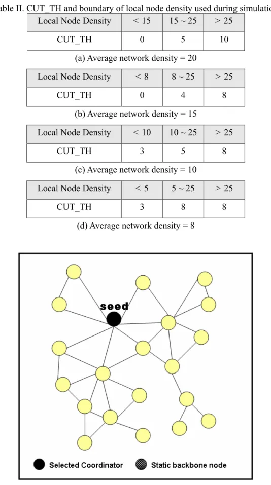
A practical example is given to explain how DDC works. If network designers deploy sensor networks with higher average network density (e.g. the average network density = 20). Three levels were applied, and the density boundaries of these three levels can be set as 15 and 25 respectively, as shown in Table II(a). CUT_CH1 was therefore applied to the nodes with local node density less than 15; CUT_CH2 was applied to the nodes with local node density between 15 and 25, and CUT_CH3 was applied to the nodes with local node density more than 25. Table II shows the

CUT_TH and local node density boundary used for different average network density during simulation. Each node maintains table 2 and operates DDC accordingly.

Table II. CUT_TH and boundary of local node density used during simulation Local Node Density < 15 15 ~ 25 > 25

CUT_TH 0 5 10

(a) Average network density = 20

Local Node Density < 8 8 ~ 25 > 25

CUT_TH 0 4 8

(b) Average network density = 15

Local Node Density < 10 10 ~ 25 > 25

CUT_TH 3 5 8

(c) Average network density = 10

Local Node Density < 5 5 ~ 25 > 25

CUT_TH 3 8 8

(a)

(b)

(d)

Fig. 2. Example of SmartBone construction

A simple example is given below to illustrate the operation of SmartBone. The backbone seeds in the network topology include the sensor gateways and the critical nodes selected via FlowBP. Figure 2(a) shows the initial topology state. SmartBone would then perform the FlowBP procedure, which finds the critical nodes from the entire topology. Critical nodes are fragile components of the network structure, so must be selected as backbone nodes. Figure 2(b) shows that node-d and node-e are critical nodes. The DFS_PRED of node-e is less than the threshold, so node-e and its correspondent, node-d, are chosen as critical nodes. The coordinators (including the critical nodes just selected) continue with backbone selecting procedure, and the neighbors of the coordinators are considered as potential candidates for the new coordinators. As shown in Fig. 2(b), node-a, node-b and node-c are on the edge of the network topology, and do not help extend the backbone. Therefore, SmartBone algorithm would not choose them as coordinators. In Fig. 2(c), assume the priorities of node-g and node-i are higher than those of other neighbors of the coordinator, so they are chosen as backbone nodes. The DDC procedure is then performed. Node-f and node-h are removed from the DDC procedure because they are too close to the selected nodes, node-g and node-i. The selection procedure is continued with node-g choosing node-j until the algorithm is completed. Figure 2(d) displays the final result.

2.3 Performance Simulation and Analysis

We adopt the ns2 [11] network simulator to evaluate the SmartBone’s performance. SmartBone was compared with SBC based on three factors: backbone size, end-to-end packet delivery ratio and energy saving ratio

2.3.1 Performance metrics

Backbone size: Backbone nodes serve nodes in the network. The backbone size

affects power consumption and interference resulting from nodes sending data. These factors are closely linked to the backbone size.

End-to-end packet delivery ratio: The Packet Delivery Ratio (PDR) indicates

the percentage of packets that can be transmitted correctly from source to destination via the backbone. The evaluating criteria of packet delivery ratio requirement differs from network applications, are discussed later.

Energy saving ratio: The Energy Saving Ratio (ESR) was derived from

dividing energy saved by backbone methods to energy consumed by the network without backbone. The ESR indicates the energy efficiency of the algorithm. Larger ESR indicates higher energy efficient.

2.3.2 Simulation Environment

The performance of SmartBone was measured with different network scenarios under different sets of source-destination pairs and node densities. A total of 100 nodes were random and uniformly distributed in varying topology sizes. In each topology, five transmission pairs were chosen with a simulation time of 300 seconds. To estimate adequately the performance of backbone construction, source and destination nodes were selected from around the topology. Information would reach the destination from source through backbone. In this simulation, the packet transmission interval was uniformly and randomly distributed between 0 and 0.3 second. Each packet size was 64 kb.

In this simulation, flooding was adopted to transmit packets between nodes. There are several reasons to choose flooding for our simulation. First, several applications need to propagate information to all nodes in sensor networks, like trigger alert notifications and query dissemination. Second, several routing algorithms

still need flooding as part of routing strategy (ex: directed diffusion). Finally, we can evaluate how the backbone reduces the collision. This is an intuition and flooding is the simplest mechanism to achieve it. The following flooding parameters were applied in the simulation. To avoid collision with packets being relayed at the same time by surrounding nodes, each receiver backed off for a random time period before relaying packets again. When receiving packets, flooding module would wait for a time interval between 0 and the maximum randomization interval, which set to 1 second in this simulation. The probability of collision depends on the Maximum randomization interval. A larger interval leads to less collision, but increases the packet delay. Thus the randomization interval is a trade-off. Furthermore, the Tx/Rx/Idle power was set to 660/395/35 mW according to ns2 default. The processing model did not consider the energy cost in CPU.

2.3.3 Simulation Results

Fig. 3. Average number of coordinators elected by the protocols during the simulation duration

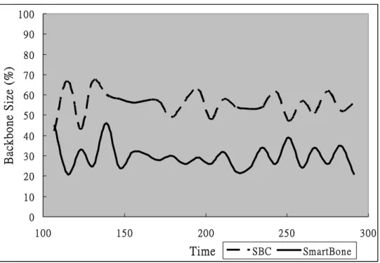
0 10 20 30 40 50 60 70 80 90 7.5 12.5 17.5 22.5 Node Density B a ck bo ne S iz e ( % ) SBC SmartBone

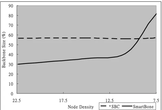
Fig. 4. Average number of coordinators elected by the protocols tests under different network density 0 10 20 30 40 50 60 70 80 90 100 7.5 12.5 17.5 22.5 Node Density P ack et De live ry Ra tio (% ) Non-Backone SBC SmartBone

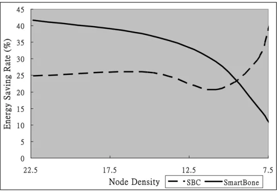
0 5 10 15 20 25 30 35 40 45 7.5 12.5 17.5 22.5 Node Density En er gy S av in g Rat e (%) SBC SmartBone

Fig. 6. Energy saving ratio tests under different network density

Figure 3 illustrates how the backbone size varies with time when using the SmartBone and SBC. The topology contains 100 nodes uniform random distributed in an 800×800 area, and the average network density is 22.5. Significantly, the size grows and shrinks over time. However, SmartBone has a backbone size of average 50% less than that of SBC, since it adopts the DDC mechanism, enabling it to delete redundant nodes more efficiently.

Figure 4 illustrates the variation in backbone size for different network density, and shows that the backbone size of SmartBone is less than SBC for network density less than 9.35. The backbone size of SmartBone maintain about half that of SBC in a topology with high network density, since the DDC is very effective. In a sparse topology (i.e. topology with low network density > 9.35), SmartBone has a much larger backbone size than SBC, because SmartBone addresses the importance of critical nodes. For a sparse topology, more critical nodes are chosen as backbone nodes to maintain necessary connectivity, so that sparse network conditions do not degrade communication. This difference is demonstrated in the packet delivery ratio graph below.

Figure 5 illustrates the performance on packet delivery ratio (PDR) in different node densities. SmartBone is compared with SBC and WSN without a backbone (i.e. every node can relay). Non-backbone method has the highest PDR at over 90%. However, this method has the highest energy consumption as expected, since every

node participates in data transmission. The PDR of SmartBone method is also over 90% for vary network density. Although, the PDR of SBC is over 90% in dense topology, SBC has a much lower PDR when the network density is sparse. We observe when network density drops to 8, the PDR of SBC is under 50%. Since SBC does not have a critical-awareness mechanism, SBC has a low PDR in sparse networks. On the contrary, SmartBone adopts the FlowBP mechanism, which takes critical nodes in the network as coordinators. Critical nodes are most important in term of network performance in sparse networks.

The reduction in energy consumption from SmartBone, and the effectiveness of SmartBone in extending the network lifetime, was investigated. Figure 6 illustrates the relationship between network density and Energy Saving Ratio (ESR). Figure 6 shows that SmartBone saves more energy than SBC, because it has a small backbone size, so more nodes are in sleeping mode. Figure 5 indicates that large number of sleeping nodes does not affect the network performance of PDR using SmartBone. More nodes are chosen as critical nodes to maintain performance in sparse networks using SmartBone. Thus, SmartBone’s energy saving will be less than SBC. In sparse case, SBC does not select critical nodes; therefore it has a smaller backbone size. A small backbone could increase radio interference and decrease the available transmission paths. Therefore, the PDR of SBC drops dramatically. Because of the PDR of SBC drops, not much transmission is success. Hence, SBC consumes less energy in the sparse networks.

2.3.4 Sensitivity of thresholds

This subsection discusses the effect of network performance on different thresholds, including the Flow threshold (FLOW_TH) and Cutback threshold (CUT_TH). The network designer must adjust these thresholds with considering the network loading, packet loss rate and delay. We provide designers with some design criteria. A PDR above 90% is considered to be the tolerant range. However, a PDR of 80% is acceptable for some applications, such as transferring temperature data. Such applications are tolerant of heavy packet loss. In such cases lower PDR is permitted, thus saving energy and ensuring that PDR is within the tolerable range.

CUT_TH is increased and FLOW_TH is decreased in dense networks, since raising CUT_TH eliminates more redundant nodes, and lowering FLOW_TH means that fewer critical nodes are selected. These two parameters help save energy by reducing the backbone size. The opposite adjustment is performed in sparse networks.

CUT_TH is reduced and FLOW_TH is increased in heavy traffic network where many backbone nodes are required to relay packets, because lowering CUT_TH means that fewer redundant nodes are eliminated, and raising FLOW_TH means that more critical nodes are selected. This resembles the trade-off between energy consumption and packet delivery ratio which give the network designers to optimize the network according to their design criteria.

Chapter 3: Minimum-Delay Energy-Efficient Source

to Multisink Routing in Wireless Sensor Networks

3.1 Introduction

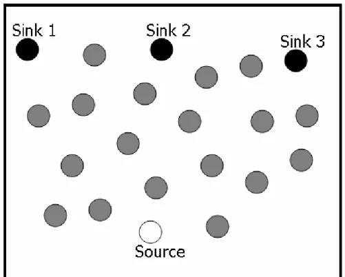
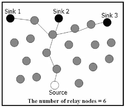
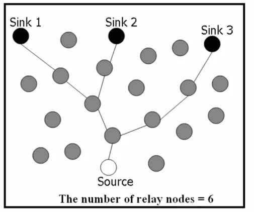
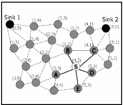
Wireless sensor network is a rapidly growing discipline, with new technologies emerging and new applications under development. In addition to providing light and temperature measurements, wireless sensor nodes have applications such as security surveillance, environmental monitoring, and wildlife watching, [20], [28], [34], and [27]. One potential application model for a sensor network is transmitting packets efficiently from Single-Source to Multi-Sinks. It’s to gather data from a single sensor node and deliver it to multiple clients who are interested in the data. This in wireless sensor network model is called Single-Source to Multi-Sinks (SSMS) [26], and is illustrated in Fig. 7. The difficulty of handling the model is in how to arrange the minimum-cost transmission path. The conventional approach is the brute force (BF) method. As shown in Fig. 8, the source finds individual paths to each sink. This approach chooses many relaying nodes (nine nodes in this example), but has the minimum transmission delay. Figure-9 shows a power-optimal solution, which has only six relay nodes. Although the energy cost of the power-optimal approach is lower than the BF method in Fig. 8, it has a larger transmission delay. Minimizing transmission delay is important, when sensor nodes inform urgent message to sinks. The best policy is to consider both energy and delay simultaneously, as illustrated in Fig. 10. The solution in Fig. 10 has only six relay nodes and a transmission delay that is as short as that of using the BF method. Hence, determining when to combine and divide packet transmission paths is a challenge. Attempts to derive an algorithm to optimize the energy consumption and the transmission delay simultaneously have so far proven futile [30]. A trade-off arises between the minimum energy cost and minimum delay. The approach presented in this section simultaneously addresses energy-cost and end-to-end delay.

SEAD [26] is a common representative solution to deal with the above SSMS problems. SEAD maintains a D-TREE (Dissemination Tree) for communication. SEAD has some drawbacks. The first drawback of SEAD is its large overhead. SEAD constructs a D-TREE for the instant source which transferring packets to the multiple sinks, and then constructs another D-TREE if another source is available to transmit packets to multiple sinks. Many sensors are available to send information to sinks in sensor networks, making the tree construction overhead excessively large. The second drawback is the large delay. A D-TREE might lower the energy consumption, but it

also prolongs the end-to-end transmission delay. Besides, FCMN [29] is another solution to handle such SSMS problems. FCMN saves energy consumption by merging multiple shortest paths for multiple sinks. It is necessary to choose the next hop nodes as the relaying nodes based on a Hop Counter Vector (HCV). Simulation showed that FCMN outperformed SEAD in term of energy consumption. However the next hop selection of FCMN is an ad hoc method. On the contrary, the next hop selection of the proposed method in this section is extended from the well-know Set Cover algorithm [31]. In order to further improve the routing performance, a Pruning Vector (PV) is introduced in this paper. The PV removes the redundant transmission paths, and further lowers the energy consumption. As a self-contained algorithm, HCR also provides a maintenance mechanism to handle the consequence of faulty nodes. Aid-TREE (A-TREE) is adopted to facilitate a restricted flooding. Moreover, Lazy-Grouping is proposed to enhance the robustness of HCR under node failure.

The rest of this section is organized as follows. Section II presents the HCR algorithm, and describes how to determine the efficient transmission path and conduct path aggregation. Section III presents the maintenance and error correction scheme of HCR, and describes the use of A-TREE to correct the inaccurate HCV resulting from failed nodes. Section IV discusses the robustness of the HCR algorithm. The proposed Lazy-Grouping algorithm is introduced and combined with HCR to produce a more robust HCR algorithm called LG-HCR, which is also compared with the original HCR. Section V presents the simulation results. HCR is also compared with other approaches in this section. Finally, conclusions are presented in Section VI.

3.2 HCR Algorithm

This section describes three main technologies of HCR, namely HCV, ESC (Extended Set Cover), and PV (Prune Vector). The proposed method assumes that each device has the same transmission range, so the connection between any two nodes is bidirectional.

3.2.1 Hop Count Vector

Each node must obtain the hop count vector only once. The following statement defines HCV of node X

HCVn(X) = { (X1,X2,...,Xn) | the hop count vector of node-X, which consists of n components,, and n denotes the total number of sinks. Each component called a hop

count value, like Xk, indicates that the hop distance from sink-k to itself is Xk hops away.}

Hence, if the network topology has only one sink, then the hop count vector has only one component. Figure-11 illustrates an example of HCV1 for sink-1, which demonstrates that each node holds one value, namely the hop distance from sink 1 to itself. Each node applies flooding to obtain the hop distance from each sink, and maintains a record of this value in HCV. A routing path with the topology with HCV1 is very simple to obtain. In Fig. 11, the hop count value of source is 4 when it transmits packets to sink-1. Therefore, the next hop has a hop count value of 3. Nodes closest to the sink have the smallest values. The rest of the next hop selection may be deduced by analogy. Finally, the packet reaches the destination correctly, and path aggregation will not be performed in this simple case.

Fig. 8. Transmission path of BF method

Fig. 10. Transmission path of the best solution

Fig. 12. Example of HCV2

HCR focuses on the case of HCVn, where n ≥ 2. The HCR algorithm must be

adopted when handling complex cases such as that of Fig. 12, which illustrates a case of HCV2(1, 2).

3.2.2 Next Hop Selection

The HCV of a node denotes the hop distance from itself to each sink. Node-X is assumed to have one neighbor node-Y, and the HCVs of the two nodes are (X1,X2,X3,...,Xn) and (Y1,Y2,Y3,...,Yn) separately. The following is a good property of HCV and the formula is proven in appendix of this paper.

|Xk-Yk||≤ 1, for any k in the range [1, n],and if node-X and node-Y are neighbor

nodes.

HCR exploits this property sufficiently to guarantee that HCR always chooses a group of nodes that are closer to the sinks.

GN(X) = { node-Y | for a node-X which HCV(X) = (X1,X2,…,,Xn), if there exists a neighborhood node-Y, which HCV(Y) = (Y1,Y2,…,Yn), and Yk < Xk, for any k where 1 ≤ k ≤ n .}

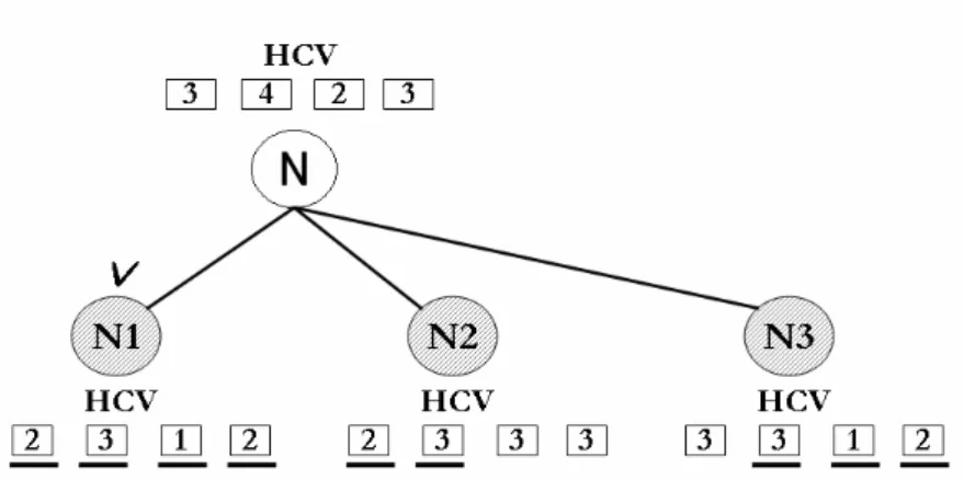
For a node-X, if node-Y is GN(X), then we can guarantee that we choose node-Y as the next hop. For example, in Fig. 13, node-N1 is a GN(N), since each component of (2,3,1,2) is less then (3,4,2,3). Hence, we choose node-N1 as the next hop, and it could approach one step closer to each sink simultaneously. However, in some case no GN(N) exists. Hence, additional neighbor nodes may be selected as the next hop. However, it will increase power consumption. The purpose of following Extended Set Cover algorithm is to choose the minimum number of nodes as the next hop. This problem can be converted perfectly into Set Cover problem [31].

Fig. 13. Example of next hop selection

3.2.3 Extended Set Cover with Load-Balance

The conventional Set Cover algorithm [31] is modified as the Extended Set Cover (ESC) scheme. ESC can efficiently select the nodes of next hop and achieve load balance. A new dimension of Set Cover Vector (SCV) is adopted to determine which neighbor node has the highest priority as the next hop. We define SCV of node X as followings:

SCVn(X) = { (X1,X2,...,Xn) | each node holds a set cover vector which consists of n components, and n denotes the total number of sinks. Each component called a set cover value, like Xk, indicates that total number of node-X’s neighbor nodes which approach one more hop toward to sink-k .}

nodes which can advance one step closer to a sink for all sinks. That information can be obtained by exchange the HCVs within neighbor nodes. If a set cover value equals to 1, the corresponding neighbor node which contributes alone to this value has the highest priority. Because only one node can approach that sink, it must be chosen as the next hop. If no set cover value is 1, then the well-know Set Cover algorithm [31] is applied. An example of the operation of ESC follows. Figure-14 illustrates seven sinks (SK1 to SK7) and five candidates (N1 to N5) for the next hop nodes. The figure indicates that N1 approaches SK1, SK2, SK3, and SK4. N2 approaches SK1, SK2, SK4, and SK5. N3, N4 and N5 have the same meaning in the figure. SK1 has a value of 3, since it is approached by three nodes, N1, N2 and N4. N3 has a highest priority as the next hop because SK7 has the set vector value of 1, meaning that only N3 can approach one hop closer to SK7. After choosing N3 as the next hop, the N3’s corresponding elements in set cover vector are updated to zero, indicating that those sinks have yet been approached by N3, as shown in Fig. 15. Therefore, the set cover vector value of each sink is checked again, and the original Set Cover algorithm is then applied to choose either N2 or N4. In Fig. 15, either N2 or N4 can cover the residual sinks, and we choose the node with more plentiful residual energy. This procedure can avoid choosing the same nodes as the next hop frequently. We assume that N4 is more plentiful residual energy than N2. Finally, in Fig. 16, two nodes (N3 and N4) are selected for the next hop in this selecting procedure. This technique is more efficient than the original Set Cover, which selects three nodes (N1, N2, and N3) in the same example.

Fig. 15. Example that after N3 is selected

Fig. 16. Final result of the next hop selecting procedure

3.2.4 Prune Vector

Figure-17 demonstrates that node-B and node-E approach the same sink, SK2, making them redundant. The same case occurs for node-A and node-F. This case contradicts the objective of the study, which is to choose the minimum number of nodes as the next hop. Therefore, a pruning algorithm based on the prune vector (PV)

is proposed.

Like HCV, the PV comprises n components, where n is the number of sinks. The component of the vector has two values, 1 and 0, denoting which sinks are pruned. If the value of component of the PV is 1, indicate that the corresponding sink has been approached by other branch of the forwarding tree. Therefore, the algorithm does not have to choose the next hop to approach the corresponding sink. Figure 18 shows an example of PV, in which node-Z picks two nodes using ESC as the next hop. Node-A approaches SK1, and node-B approaches SK2. Hence, node-Z sets the pruning bit of SK2 to 1, and notifies node-A. At the same time, it sets the pruning bit of SK1 to 1 and notifies node-B. Since PV has the property of inheritance, which means that if one node prunes some sinks, then all its children also prunes the same sinks as illustrated in Fig. 18. Therefore, if one node has the values of PV all equal to one, the node can be pruned such as Node-E and Node-F in Fig. 18. Since no matter the node approaches to which sinks, it all has been covered by other forwarding branches. HCV with PV can further reduce redundant nodes for relaying.

Fig. 18. Example of PV

3.3 HCR Maintenance Scheme

This section discusses the maintenance scheme of HCR, including the detection of a failure node, and determining a flooding scope in order to update inaccurate HCVs due to a node failure. We finds out these nodes within the flooding scope using an tree structure called Aid-TREE, and performs limited flooding. The following subsection elucidates these technologies.

3.3.1 Flooding Scope

The relevant terms are formally defined as follows:

Base-HCV(X, k) = { (true, false) | for node-X where HCV(X) = (X1,X2,…,Xn), if Xk = 0, then the value of Base-HCV(X, k) is true. Otherwise, if there exists node-Y and HCV(Y) = (Y1,Y2,…,Yn), Yk < Xk, then the value of Base-HCV(X, k) is true, else the value is false. }

Accurate-HCV(X) = { (true, false) | for node-X where HCV(X) = (X1,X2,…,Xn), if the value of Base-HCV(X, k) equals true for any k in the range [1,n], then the value of Accurate-HCV(X) is true, otherwise the value of Accurate-HCV(X) is false. }

Each node broadcasts the hello message periodically, informing neighbor nodes that it is still alive. Each node simultaneously checks whether its Accurate-HCV value was true. If Accurate-HCV(X) is true, then node-X has an accurate HCV. Otherwise, node-X has an inaccurate HCV. A failure may lead to some nodes with inaccurate HCVs, and results in the HCV correcting algorithm being applied. The HCV of each node is obtained when hop count information is exchange by flooding after deploying the sensor network. Hence, the flooding is performed again to obtain the correct HCV. However flooding has a very high overhead, and only a few network nodes need to be corrected. Therefore, an efficient correction mechanism is proposed to correct the inaccurate HCVs. We define the flooding scope as follows:

Flooding scope = { {node-X} | node-X has the inaccurate HCV. }

The HCVs of the nodes within the flooding scope must be corrected, while nodes outside the flooding scope have accurate HCVs. Therefore, the objective is to determine the flooding scope and perform the limited flooding.

The terminal node (TN) is defined as follows:

TN = { {node-X} | there exists a link between node-X and node-Y, where node-X is outside the flooding scope and node-Y is inside the flooding scope. }

The goal can be reduced to just finding TNs, from which the limited flooding can be applied and inaccurate HCVs can be updated. This is because the maximum flooding scope is bounded by TNs. Aid-TREE (A-TREE) is proposed to identify the TNs, and is explained in the next subsection.

3.3.2 Aid-TREE

We define the beginning node (BN) as follows:

BN(k) = { {node-X} | for a node-X, which satisfies that its kth component of HCV is inaccurate and it is direct adjacent to the failed node. }

Since the node adjacent to the failed node could find itself as BN, BN is the root of Aid-TREE. The correcting mechanism will repair each inaccurate component by broadcasting the information containing the value of its inaccurate component plus

one, as illustrated in Fig. 19. The nodes then receive the message, and check that its relative component corresponds to the message, if they are equal, in which case the value of the components increase one and forwards the value to its neighbors again. Otherwise, the node sets itself as TN, as illustrated in Fig 20. In the second phase, TN notifies backwardly the node if it has larger component value than TN, and the node sets itself as a new TN like the shaded node in Fig. 21. Otherwise, the TN remains as a TN. The procedure is repeated until all TNs are discovered. Figure-21 displays the final result of A-TREE, and Fig. 22 shows the flooding scope bounded by the TNs. The restricted flooding is then performed starting from all TNs, and finally the topology has the correct HCV information.

Fig. 19. Operation of finding an A-TREE

Fig. 21. The second phase of finding an A-TREE

Fig. 22. A final A-TREE

3.4 Robustness Improvement

This section explores the impact of the failed node caused by either battery run out or malfunctions. Failure nodes may occur at any time, causing sensor nodes to have the wrong HCVs. Fortunately, it’s not necessary to correct HCVs in most cases where a failed node occurs.

HCR has made significant improvement in robustness with A-Tree and limited flooding. Lazy Grouping (LG) is proposed to cooperate with original HCR (called LG-HCR) to further improve the robustness. Figure-23 shows an example of the LG method. To choose appropriate sensors from network to group the nodes, each node must be prioritized. Many methods are available for setting node priorities [32]. HCR adopts the simplest method, in which the priority of a node is determined from its remaining energy. The node with the highest priority initially acts as group leader, and it notifies its neighborhood within a two-hop range. These neighbors receive the message, and accurately set the corresponding group leader. Repeating the process, a group leader is generated from the nodes that haven’t been grouped, and notifies the related group members, as shown in Fig. 23. The whole network applies the HCV assignment to each group, therefore, for the nodes within the same group will hold the same hop count value. Fig. 23 shows the result of conducting the LG method. When we route data from a source to multiple sinks in the Lazy Groups, we apply the same HCR algorithm to the virtual topology derived from original network topology as shown in Fig. 23. Instead of directly forwarding data to the next hop, a node should forward data to its group leader first. The group leader will be responsible to forward data to the next group according to the rule of HCR until the destinations have been reached. For example, in Fig. 23 node-D in group with the HCV labeled as 2 (namely group-2) would like to transmit packets to Node-C with the HCV labeled as 3 (Group-3), node-D first queries its group leader that how to reach group-3. Then node-D gets the routing information from its group leader and transmits the packets to group lead of Group 3, and then to node-C. Therefore, it prolongs the transmission delay.

Fig. 24. Network topology without LG

Fig. 25. Network topology with LG

The reason why LG improves robustness is explained below. Figure-24 illustrates the same topology as in the previous example without LG and with HCV assignment. Node-A, node-B and node-C have HCVs of 4, 5 and 6, respectively. If node-A has failed, then node-B and node-C both have inaccurate HCVs. Therefore, these two nodes should run correcting algorithms and update the inaccurate HCVs. On the contrary, in Fig. 25, the original node-A, node-B and node-C have HCV values of 2, 3 and 3, respectively. The left-hand side of Fig. 25 represents the LG topology,

which can be regarded as the virtual topology as in the right-hand side. The LG topology has high connectivity among neighbor groups, because each group has lots of links to its neighbor groups. Therefore, the HCV has slightly effects due to the failed nodes, as shown in Fig. 25. Nodes in the group with a HCV labeled as 2 may reach node-E, which the HCV labeled as 3, through node-D, and irrespective of the failed node-A. Hence, LG can reduced the frequency of HCV update and improve the robustness of HCR routing in sensor networks.

3.5 Simulation Results and Performance Analysis

The performance of a routing algorithm is usually evaluated according to connectivity, energy consumption, throughput and robustness [33]. To evaluate the HCR protocol, three main categories, energy consumption, robustness, and delay were adopted in this section to compare HCR with BF and FCMN [29] methods. These routing algorithms were simulated using C++ programs. The task of sensor nodes is to gather data and deliver it to multiple clients who are interested in the data. In our assumption, the simulation traffic is not heavy loading. It is reasonable because of the transmission properties of sensor nodes. Hence, the influence with contention and collision is negligible.

3.5.1 Performance metrics

Energy consumption: The total number of transmissions was adopted to

evaluate the energy cost. The numbers of transmissions in HCR, BF and FCMN were compared by varying the network topology. The number of relay nodes equals the total number of transmission. Many transmissions imply a high energy cost.

Robustness: The network topology had 400 nodes with IDs assigned from 1 to

400. The original HCR was compared with LG-HCR in term of robustness. The robustness of algorithm was evaluated using the following parameters.

Total number of NTR: Each node-k where k was looped from 1 to 400 was made to fail in turn, and the number of times each failed node resulted in inaccurate HCVs among its neighbors was recorded. If the failed node affected its neighbors’ HCVs and the topology became 'Need to Repair' (NTR), then the total number of NTR was increased by one. In the worst case, the number of NTR equals to 399 (the number of nodes of entire network minus 1), which means that some of the HCVs have to be updated each time a node fails. A small NTR value indicates a high robustness.