以時間解析飛秒光譜研究六方晶系結構鈥錳氧單晶之載子動力學

國立交通大學

電子物理學系

博士論文

以時間解析飛秒光譜研究六方晶系結構

鈥錳氧單晶之載子動力學

Study of the Carrier Dynamics in Hexagonal

HoMnO

₃

Single Crystals Using Time-Resolved

Femtosecond Spectroscopy

研 究 生 ：石訓全

指導教授 ：吳光雄 教授

羅志偉 教授

以時間解析飛秒光譜研究六方晶系結構鈥錳氧

單晶之載子動力學

Study of the Carrier Dynamics in Hexagonal HoMnO

3

Single

Crystals Using Time-Resolved Femtosecond Spectroscopy

研 究 生：石訓全 Student：Hsun-Chuan Shih

指導教授：吳光雄 教授

Advisor：

Prof. Kaung-Hsiung Wu

羅志偉 教授

Advisor：

Prof. Chih-Wei Luo

國立交通大學

電子物理學系

博士論文

A Dissertation

Submitted to Department of Electrophyscis

College of Science

National Chiao Tung University

in Partial Fulfillment of the Requirements

for the Degree of

Doctor of Philosophy

in

Electrophysics

July 2010

Hsinchu, Taiwan

中華民國九十九年七月

以時間解析飛秒光譜研究六方晶系結構鈥錳氧

單晶之載子動力學

研究生：石訓全 指導教授：吳光雄 教授

羅志偉 教授

國立交通大學 電子物理學系

中文摘要

在本論文中，我們利用具有時間解析的激發探測實驗去研究多鐵性六

方晶系鈥錳氧單晶的超快載子動力學。首先，我們量測六方晶系鈥錳氧單

晶的基本特性，例如用

X 光 θ-2θ 繞射確認晶體結構及用超導量子干涉儀進

一步確定磁矩隨溫度的排列情形。在此材料系統中，所謂＂多鐵＂是指具

有電性(鐵電)與磁性(反鐵磁)以及彈性等多個有序特性的共存，且在該材

料中磁電、磁彈間存在著強的耦合(Coupling)作用，即施加電場可影響磁性，

反之加磁場又可影響其電的特性。這些有序參數間的交互作用引發許多的

有趣現象，近年來引發科學家的研究熱潮。

從激發探測實驗結果中，透過波長可調的飛秒光譜實驗在鈥錳氧單晶

中觀察到反鐵磁有序與電子結構會有強烈的耦合情形，該材料中存在的磁

長程有序會造成錳離子

3d 軌域在尼爾溫度有異常的藍移現象，同時在尼爾

溫度之上因短程有序的出現造成反射率變化(R/R)的振幅對溫度變化之斜

率有顯著的改變。接著，我們在鈥錳氧單晶中透過激發光所造成的光致熱

彈效應(thermoelastic effect)在尼爾溫度觀察到異向性的磁彈耦合行為，進而

揭示了電性、彈性與磁性不同自由度間的耦合情形。其中光致熱彈效應在

ab 平面上造成反射率變化被我們定義的”負”分量所主宰，而沿著 c 方向傳

遞的應力形變波則造成反射率變化中的”振盪”分量，兩個分量皆在尼爾溫度

出現異常的變化。最後，從反射率變化中的振盪分量隨溫度的變化，我們

認為週期的變化來自於鐵電的極化率隨溫度的改變。

Study of the Carrier Dynamics in Hexagonal

HoMnO

₃

Single Crystals Using Time-Resolved

Femtosecond Spectroscopy

Student：Hsun-Chuan Shih Advisor：

Prof. Kaung-Hsiung Wu

Prof. Chih-Wei Luo

Department of Electrophysics

National Chiao Tung University

Abstract

In this dissertation, we study the characteristics of ultrafast carrier

dynamics in hexagonal HoMnO

3

single crystals via time-resolved pump-probe

experiments. First of all, we measured the fundamental properties of hexagonal

HoMnO

3

, such as crystal structure by the X-ray diffraction (XRD) θ-2θ pattern,

the arrangement of magnetic moment by the superconducting quantum

interference device (SQUID). Multiferroic materials with coexistence of several

ferroic orders (ferroelectric, ferromagnetic, or ferroelastic) have attracted great

attention of scientists recently. The magnetoelectric response is the appearance

of an electric polarization upon applying a magnetic field and/or the appearance

of a magnetization upon applying an electric field.

In pump-probe results, we demonstrate that the strong coupling between

the electronic structure and antiferromagnetic (AFM) ordering in hexagonal

HoMnO

3

single crystals can be simultaneously delineated by

wavelength-dependent femtosecond spectroscopy. The emergence of long-range

and short-range magnetic ordering are unambiguously revealed in association

with an abnormal blue-shift of Mn

3+

3d level around the Néel temperature and

the slope change of the temperature-dependent ΔR/R near transition, respectively.

Furthermore, the coupling among the magnetization, polarization, and strain

degree of freedoms has been simultaneously disclosed in the hexagonal

HoMnO

3

single crystals through the photo-induced anisotropic ultrafast

thermoelastic dynamics. The thermoelastic effect in the ab-plane associated with

the giant magnetoelastic coupling around the Néel temperature (T

N

) is intimately

correlated to the evolvement of a negative component in the transient reflectivity

changes (R/R) obtained from temperature-dependent pump-probe experiments.

Moreover, the variation of the period of the oscillation component in ∆R/R

caused by a strain pulse propagating along c-axis exhibits an abrupt drop around

Acknowledgments

回想起四年多前，決定參與研究中心實驗室的成立與建置，現在回頭想想這還真是 個正確的決定，因為這個經驗讓我學到太多的東西了。這條漫長研究的道路上有責任有 壓力，有成就有收穫，其中的難過與開心則是點滴在心頭。最後用＂值得＂來替自己的 博士生涯做最佳的註解，這也會是一段最讓我難忘的人生旅程。 博士四年的經歷與些許的成就建立在辛勤的耕耘，但是過程中因為有太多人的協助 與關心才有這一點點成績讓我以後可以驕傲的拿出來說嘴。有很多感謝的話，首先，我 的指導老師與共同指導老師：吳光雄教授與羅志偉教授，謝謝你們對我的信任與對我的 包容，在三更半夜還陪我討論實驗與論文，對於研究的態度與堅持著研究的熱忱更是讓 我大開眼界；固態實驗室的老師群：溫增明教授、莊振益教授、林俊源教授、郭義雄教 授，雖然每次 Meeting 都遭受無情的炮火襲擊，但不可諱言這是讓我成長最直接的方法， 並且讓我釐清我的思緒與方向，特別是能得到溫老師的些許肯定更讓我備感榮幸；莊院 長謝謝你常常在百忙之中幫我修改論文，讓我的論文更加完備；超快研究中心的小林孝 嘉教授、籔下篤史教授，沒有你們提供如此完善的研究設備難以成就這本論文。 再來就是感謝實驗室的夥伴了! 謝志昌學長與宗漢，要不是有你們在我低潮遭遇困 難的時候拉我ㄧ把，給我協助與幫忙，我想今天也就不會在這邊寫誌謝了。另外要感謝 信斌、龍羿、育賢，實驗室建立之初就是我們胼手胝足，一起努力才有現在實驗室的規 模。還有這個大家庭裡許許多多的學弟妹：新安、以恆、純芝、享穎、昱庭、宣懿、維 聰、劭軒、潤東、裕廉、志翔、佳璟、易修、韋臻、志賢、文彥等，平常陪我吵吵鬧鬧、 裝瘋賣傻、互相幫忙，好不開心! 除此之外，也有許多曾經在我博士生涯中出現的好朋 友對我的鼓勵與支持更是我完成博士學位的最大動力，令人難忘。

當然拿到博士學位，最感謝的是我的父母與哥哥，沒有你們全力的支持與栽培，沒 有今天的我，家裡大大小小的事情都不需要我來分擔，讓我無後顧之憂完成我的學位。 現在要離開實驗室了，心情自然是百感交集。如今的我帶著滿滿的成就與回憶，就 像當初空蕩蕩的實驗室現在則是填滿了許許多多的儀器，希望帶著一身練就的武功到外 面的世界闖一闖，能讓實驗室以我為榮!

Table of Contents

Abstract (in Chinese)

i

Abstract (in English)

iii

Acknowledgements

v

Table of Contents

vii

Chapter 1 Introduction

1

1.1 Survey the researches of hexagonal ReMnO

3

materials

7

1.2 Motivation

12

1.3 The organization of this dissertation

14

Chapter 2 Experimental tools and procedures

19

2.1 Characterization and preparation of h-HoMnO single crystals

19

2.1.1

Orientation and structure of HoMnO

3

single crystals

20

2.1.2

Temperature-dependent susceptibility measurements

22

2.1.3

Transmittance spectrum

24

2.2 Femtosecond time-resolved systems

26

2.2.1

The polarized femtosecond pump-probe system

27

2.2.2

The terahertz time-domain spectroscopy

29

2.2.3

The optical pump terahertz probe system setup

32

Chapter 3 The femtosecond pump-probe spectroscopy

39

3.1 The characteristics of femtosecond pulse laser

39

3.1.1 The light pulses

40

3.1.3 Measurement of the pulse temporal profile

44

3.2 The fundamental principle of pump-probe experiments

47

3.3 The coherent spike in reflection-type pump-probe

49

Chapter 4 The ultrafast dynamics on h-HMO single crystals

56

4.1 The results of ∆R/R at various wavelengths and temperatures

57

4.1.1

The transient reflectivity changes ∆R/R

57

4.1.2

Classify the ultrafast behaviors in ∆R/R curves

60

4.1.3

The mathematical fittings in ∆R/R curves

62

4.2 The temperature-dependent amplitude of ∆R/R

65

4.2.1

The amplitude of ∆R/R between 20-300 K

65

4.2.2

The amplitude of ∆R/R in high temperature range

70

4.3 The anisotropic magnetoelastic coupling in h-HMO

72

4.3.1

Laser-induced thermoelastic generation

72

4.3.2

Laser-induced lattice dynamics on a-b plane

74

4.3.3

Laser-induced strain pulse propagation along c-axis

81

Chapter 5 Summary

92

Chapter 1

Introduction

Multiferroic materials [1-5] with coexistence of various ferroic orders (ferromagnetic, ferroelectric, or ferroelastic) have attracted great attention in condensed-matter researches due to their great potential for applications in the field of oxide electronics, spintronics, and even the green energy devices for reducing the power consumption. In multiferroic oxides (in single phase), the coupling interaction among various order parameters causes the magnetoelectric (ME) effect [6-11]. Namely, a polarization (magnetization) can be induced by application of a magnetic (electric) field. Although the properties of electricity and magnetism

were combined into one common discipline by Maxwell equations in the 19th century, the

electric and magnetic orderings in solid-state materials is always considered separately. This is because that the electric charges of electrons and ions are responsible for the charge effects, whereas the electron spins govern the magnetic properties.

The presaging of a strong coupling between magnetic and electric degrees of freedom in one substance can be traced back to very long time ago which was provided by Pierre Curie

with a short comment in Landau and Lifshitz’s course of theoretical physics [13]:

“Let us point out two more phenomena, which, in principle, could exist. One is piezomagnetism, which consists of linear coupling between a magnetic field in a solid and a deformation (analogous to piezoelectricity). The other is a linear coupling between magnetic and electric fields in a media, which would cause, for example, a magnetization proportional to electric field. Both these phenomena could exist for certain classes of magnetocrystalline symmetry. We will not however discuss these phenomena in more detail because it seems that till present, presumably, they have not been observed in any substance.”

Thereafter, this short remark about the linear magnetoelectric coupling effect was changed soon due to the prediction of Dzyaloshinskii [14] and the observation of Astrov [15].

Dzyaloshinskii, a condensed-matter physicist in Russia, predicted that the Cr2O3 crystals

satisfy the conditions of magnetoelectric effect in 1959. In next year 1960, Astrov

successfully observed the magnetoelectric effect in the Cr2O3 single crystals. From that time,

the magnetoelectric materials attracted great attention and caused strong studies. During several years, then, many kinds of magnetoelectric materials had been discovered, such as

Ti2O3 [16], Ni3B7O13 [17], BiFeO3 [18], GaFeO3 [19], Y3Fe5O12 [20], and etc.. Unfortunately,

these upsurged studies declined gradually due to that the magnetoelectric coupling coefficient is too small to the applications which were highly praised by scientists at that time.

Until 2000, the studies of the perovskit-based multiferroic materials, such as rare-earth

manganates TbMn2O5, YMnO3, BiMnO3, etc., renewed the scientists’ attention and began all

over again. There are two main reasons: the first one is the breakthrough of the theoretical works which are due to the combination between the developments of density functional

theory and the technology of computer [21]. On the other hand, it is due to the improvement in thin film deposition. Thus, the artificial thin films can be produced to match the requirements of theoretical works.

Figure 1-1 shows the relationship between multiferroic and magnetoelectric which tells us the fact that there are few materials belongs to multiferroic materials. Although it is not easy to find new multiferroic materials, there are still a lot of multiferroic materials that had been discovered and investigated recently. In order to understand the physical mechanism of multiferroic materials, W. Priller et al. [22] classified the characteristics of multiferroic

materials into three categories. The first one is Bi-based compounds, such as BiMnO3, BiFeO3,

and PbVO3, etc.. The second one is other perovskites and related materials: ReMnO3

compounds (Re = Y, Ho, Er, Tm, Yb, and Lu). The third one is ReMn2O5 (Re = rare-earth).

The aim of his paper is to introduce the current materials which are under study. Addtionally, S.-W. Cheong et al. [23] further summarized the classification of “proper” and “improper” ferroelectrics shown in Table 1.1 by the mechanism of ferroelectricity. In the category of the

Figure 1-1: The relationship between multiferroic and magnetoelectric

proper ferroelectrics, the main driving force toward the polar state was associated with the electronic pairing. In contrast, the induced polarization of ferroelectricity involves a more complex lattice distortion or other accidental by-product of some other ordering is called

“improper” [24], such as the hexagonal manganites ReMnO3 which show a lattice distortion

to enlarge their unit cell (geometric ferroelectricity) [25-27]. Moreover, another group of improper ferroelectrics are those induced by magnetic ordering.

In this dissertation, we will focus on the “improper” ferroelectric materials which are

geometric ferroelectrics ReMnO3. The multiferroic rare-earth manganites (ReMnO3) have

attracted great scientific attention since the manifestations of the intriguing and significant coupling between the magnetic and electric order parameters. The coexistence of ferroic

orders in ReMnO3 with hexagonal (smaller ionic radius of rare-earth Re = Sc, Y, and Ho-Lu)

or orthorhombic (larger ionic radius of rare-earth Re = La-Dy) (shown in Fig. 1-2) structure not only gives the rich physics in the intimate interactions among charge, orbital, lattice, and spin degrees of freedom but also possesses some fascinating physical properties which might

lead to the potential applications. As indicated in Table 1.1, ReMnO3 has two kinds of

ferroelectric behaviors (hexagonal or orthorhombic) induced via different originations. The Table 1-1: The classification of ferroelectrics: proper and improper ferroelectricity [23]

rare-earth (Re3+) ionic size decreases from 1.11 Å to 0.94 Å with decreasing the atomic number and reducing the electrons residing in the 4f orbit which formed the so-called

lanthanum contraction effect [28]. The Re3+ ions of the rare-earth elements have closely

chemical properties because the outermost electrons with the same 5s25p6 electronic

configurations, like neutral xenon. The orthorhombic structure with Pnma space group is the

stable crystal structure of ReMnO3 perovskite oxides with Re = La to Dy, which belongs to the

magnetic ferroelectrics induced by magnetic ordering [29-36]. On the other hand, another group of compounds with small ionic size (for Re = Y, Ho, Er, Yb, Lu, and etc.) forms the

stable hexagonal structure with P63cm space group. The critical point of the structure

transition locates near YMnO3 (Y3+ =1.06Å) and HoMnO3 (Ho3+ = 1.05Å). Consequently, the

crystal structures of those two compounds have been transformed from hexagonal to orthorhombic (or vice versa) by a lot of experimental techniques, e.g. high temperature and high pressure processes [37-38], chemical solution deposition (CSD) [39], the metal-organic chemical vapor deposition (MOCVD) [40], molecular beam epitaxy (MBE) [41], sputtering [42], and pulsed laser deposition (PLD) [43].

Figure 1-2: The evolution of the lattice structure in ReMnO3 as a function of

In the following sections, we are going to change the point of view which is from the development of history to the recent researches of the multiferroic hexagonal manganites

(ReMnO3). Due to the effect of geometric structure, the magnetic frustration appears in the

improper ferroelectricity in ReMnO3. Thus, we are interested in the interactions among the

charge, lattice, and spin degrees of freedom in this kind of strong correlated system. Furthermore, we will present the motivation of our study in the hexagonal manganites.

1.1 Survey the researches of hexagonal ReMnO

3

materials

The hexagonal ReMnO3 (Re = rare-earth) materials show the similar properties among

various rare-earth elements, whether the properties of electric transportation or magnetic

behaviors. Following, our discussions will focus on the properties of the hexagonal HoMnO3

(h-HMO), because h-HMO is an intriguing multiferroic. The hexagonal HoMnO3 is with the

ferroelectric ordering at Curie temperature TC = 875 K, the antiferroicmagnetic (AFM) Mn3+

ordering at Néel temperature TN = 76 K, and the magnetic Ho3+ ordering at THO = 4.6 K, in

which the magnetically active ions are the high spin Mn3+ (3d4, S = 2) and Ho3+ (4f10)

(ground-state multiple 5I8) [6, 26, 44-50]. Fig. 1-3 (a) and (b) show the crystal structure of

hexagonal ReMnO3 at paraelectric (P63/mmc) and ferroelectric (P63cm) phase, respectively

[51].

Figure 1-3: Schematic crystal structures of ReMnO3 in hexagonal structure. (a)

What is the origin of the ferroelectricity in magnetoelectric ReMnO3? B. B. van Aken et al. [26] reported the ferroelectric phase transition in the hexagonal manganite YMnO3 through

the detailed structure analysis from x-ray diffraction and the first principle density functional

calculations. The ferroelectric phase is characterized by a buckling of the layered MnO5

polyhedra and accompanied by the displacements of the Y ions, which lead to a net electric polarization. Similar results had been shown by Th. Lonkai et al. [52]. Fig. 1-4 shows the

“geometric” generation of polarization in YMnO3 and describes the tilting of a rigid MnO5

block with a magnetic Mn atom at the center.

Figure 1-4: Schematic crystal structure of YMnO3. Arrows indicate the

directions of the atomic displacements moving from the centrosymmetric to the ferroelectric structure [26].

Polarization along c-axis

The magnetic structures of h-HMO have been studied by various experimental methods, such

as neutron diffraction [50, 53] or second harmonic generation (S.H.G.) [45, 54]. In the P63cm

hexagonal phase, each Mn3+ ion is surrounded by five O2- ions and formed triangular planar

sublattices in the basal plane (a-b plane). The magnetic order of Mn3+ is mainly dominated by

AFM in-plane Mn-O-Mn superexchange interaction. Therefore, the triangular lattice of the Mn atoms exhibits strong geometrical frustration effect [55]. Furthermore, when temperature

cool to near TN, the strong superexchange leads to a 120° arrangement between neighboring

Mn3+ spins in the basal plane which breaks the triangular frustration. In addition, the spins of

Mn rotate with an angle of 90° at TSR (e.g. for h-HoMnO3, TSR ~ 33 K) due to the onset of the

AFM order of the Ho moments indicating that the interaction between Ho3+ and Mn3+ spins.

Another magnetic transition at THO ~ 5 K involves with the complete magnetic order of the

Ho3+ ions. These spin arrangements at different temperatures are shown in Fig. 1-5.

In addition to the basic properties of ferroelectricity and magnetization, in 1997,

(a)

T > T

SR (b)

T < T

SR (c)

Figure 1-5: Scheme of the magnetic structure of HoMnO3: (a) TSR < T < TN, (b)

Huang et al. [56] have reported that the anomaly of the dielectric constant at Néel temperature

(TN) which is due to the coupling between the ferroelectric and antiferromagnetic order

parameters (the arrow in Fig. 1-6 (a)). Moreover, during 2004-2005, B. Lorenz et al. observed

a reentrant phase in the hexagonal ferroelectric HoMnO3 below the temperature of so-called

spin rotation (TSR) shown in Fig. 1-6 (b). Under applied magnetic fields, HoMnO3 exhibits

complex T-H phase diagram with several field-induced reentrant phases and transitions at low temperatures shown in Fig 1-6 (c) [57-59].

Figure 1-6: (a) There are two anomalies behaviors shown in the low

temperature dielectric constant. (b) The dielectric constant plotted as a function of temperature with several external magnetic fields. (c) The low temperature T-H phase diagram of HoMnO3 [57-59].

(c)

The magnetoelectric coupling in HoMnO3 will be discussed in chapter 4 of this dissertation.

Briefly, the anomalous dielectric constant at TN along c-axis in hexagonal ReMnO3 has been

assigned to the indirect coupling via lattice strain (spin-lattice coupling). Moreover, there are

many researches show that the abnormal behavior at TN, such as the heat capacity

measurements, the lattice constant measurements, and etc., which are shown in Fig. 1-7(a) and (b) [58, 60-61].

Very recently, Lee et al. [62] observed the giant magnetoelastic effect in hexagonal YMnO3

and LuMnO3 by using the high-resolution neutron and synchrotron powder diffraction

experiments (shown in Fig. 1-8). They further claimed that the magnetoelectric (ME)

coupling can be interpreted by the giant magnetoelastic effect very well in ReMnO3, i.e. the

magnetic long-range ordering induced the very large displacements of all atoms at Néel temperature. In other words, the magnetoelastic coupling let the atoms undergo an isostructural transition, which has been regarded as the primary source of the ME phenomena.

In hexagonal ReMnO3, this magnetoelastic effect is two orders of magnitude larger than those

Figure 1-7: (a) Theλ-type anomaly around TN in the specific heat of HoMnO3.

(b) The temperature–dependent lattice constant along a- and c-axis [60-61].

appeared in other magnetic materials. Therefore, the gigantic magnetoelastic coupling plays a

crucial role to dominate a lot of physical properties in hexagonal ReMnO3.

1.2 Motivation

The previous research results as mentioned above show the rich physical phenomena in

hexagonal ReMnO3 multiferroic materials caused by the strong interaction among charge,

lattice, and spin degrees of freedom. N. A. Spaldin and M. Fiebig further proposed the strong coupling among the electric polarization (P), magnetization (M), and strain (ε). Also, one of them can be changed by driving the other physical parameters [63] as shown in Fig. 1-9. Thus,

to understand the strong interaction among different order parameters in hexagonal ReMnO3

multiferroic materials must be a key issue.

Figure 1-8: (a) The model shows how Mn atoms (large blue circles) move

below TN with respect to O3 atoms (small orange circles). (b) Temperature

dependent of the Mn x position and the Mn-O bond distances [62].

(a)

(b)

O3 Mn

Our motivation is to understand the correlation among different degrees of freedom by pump-probe spectroscopy with femtosecond time-resolution. Through the pump-probe spectroscopy, we can observe the rapid responses in materials, such as the relaxation time of the excited electrons from excited state to ground state in several picosecond. Thus, the

intricate correlation processes among the charge, lattice, and spin degrees of freedom can be

Time‐resolved pump‐probe spectroscopy  The strong correlation between  charge, lattice, orbital, and spin  degrees of freedom.  Femtosecond laser pulse  Electrons Spin Electrons Lattice τe‐s  Spin τe‐p  τl‐s 

Figure 1-10: The flow chart of our motivation. Utilize the ultrashort pulse laser

as a tool to investigate the strong correlation between different kinds of degrees of freedom.

Figure 1-9: The electric field E, magnetic field H, and stress σ control the

explicitly recognized in different characteristic time scales by measuring the transient reflectivity or transmittance. From the ultrafast dynamical spectroscopy, the microscopic mechanism of the magnetoelectric coupling or magnetoelastic behavior can be revealed.

1.3 The organization of this dissertation

This dissertation consists of five chapters. In chapter 1, we simply introduce the multiferroic materials and magnetoelectric coupling phenomena. The motivation of this study is also included. In chapter 2, we give a brief introduction to the growth of high quality samples. Moreover, the crystal structures and orientations of all samples were examined by x-ray diffraction (XRD). The magnetic properties of all samples were inspected by a Quantum

Design® superconducting quantum interference device (SQUID) system. The other focal

point in chapter 2 is the system setup of the ultrafast femtosecond pump-probe and described in details. In chapter 3, we are going to discuss the fundamental principle of pump-probe technique. First, we present the fundamental physics in ultrashort pulse laser. Next, we discuss the principle of time-resolved pump-probe spectroscopy. Finally, we focus on the origin of the coherent spike signals induced by two laser beam interference. In chapter 4, we present all of the pump-probe experimental results. The pump induced dynamics of electrons, holes, and phonons are influenced by their interaction with each other. We demonstrate and explain that

the ultrafast dynamics of electrons and lattice in hexagonal HoMnO3 (h-HMO) single crystals.

In the pump-probe experiments, we observed the dynamical behavior of electrons coupling

with antiferromagnetic (AFM) ordering at Néel temperature (TN) which is magnetoelectric

coupling. Moreover, through the ultrafast lattice dynamics we directly observed the giant and

anisotropic magnetoelastic coupling at TN on a-b plane and along c-axis. In chapter 5, we

References

[1] H. Schmid, Ferroelectrics 162, 317 (1994). [2] M. Fiebig, J. Phys. D 38, R123 (2005).

[3] C. W. Nan, M. I. Bichurin, S. Dong, and D. Viehland, G. Srinivasan, J. Appl. Phys. 103, 031101 (2008).

[4] D. Khomskii, Physics 2, 20 (2009).

[5] W. Eerenstein, N. D. Mathur, and J. F. Scott, Nature (London) 442, 759 (2006).

[6] T. Lottermoser, T. Lonkai, U. Amann, D. Hohlwein, J. Ihringer, M. Fiebig, Nature 430, 541 (2004).

[7] B. Lorenz, Y. Q. Wang, and C. W. Chu, Phys. Rev. B 76, 104405 (2007).

[8] B. Lorenz, Y. Q. Wang, Y. Y. Sun, and C. W. Chu, Phys. Rev. B 70, 212412 (2004).

[9] T. Kimura, T. Goto, H. Shintani, K. Ishizaka, T. Arima, and Y. Tokura, Nature. 426, 55 (2003).

[10] M. Fiebig, T. Lottermoser, D. Frohlich, A.V. Goitsev, and R.V. Pisarev, Nature 419, 818 (2002).

[11] N. Hur, S. Park, P. A. Sharma, J. S. Ahn, S. Guha, and S.-W. Cheong, Nature 429, 392 (2004).

[12] P. Curie, J. Physique 3, 393 (1894).

[13] L. D. Landau and E. M. Lifshitz, Electrodynamics of continuous media (Fizmatgiz, Moscow) (1959).

[14] I. E. Dzyaloshinskii, Sov. Phys. JETP 10, 628 (1959). [15] D. N. Astrov, Sov. Phys. JETP 11, 708 (1960).

[16] B. I. Alshin and D. N. Astrov, Sov. Phys. JETP 17, 809 (1963).

[17] E. Ascher, H. Rieder, H. Schmid, and H. Stoessel, J. Appl. Phys. 37, 1404 (1966).

Comm. 7, 701 (1969).

[19] G. T. Rado, Phys. Rev. Lett. 13, 335 (1964).

[20] B. B. Krichevtsov, V. V. Pavlov, and R. V. Pisarev, JETP Lett. 49, 535 (1989). [21] N. A. Hill, Annu. Rev. Mater. Res. 32, 1 (2002).

[22] W. Prellier, M. P. Singh, and P. Murugavel, J. Phys.: Condens. Matter 17, R803 (2005). [23] S. -W. Cheong and M. Mostovoy, Nature Mater. 6, 13 (2007).

[24] A. P. Levanyuk and D. G. Sannikov, Sov. Phys. Usp. 17, 199 (1974).

[25] T. Katsufuji, S. Mori, M. Masaki, Y. Moritomo, N. Yamamoto, and H. Takagi, Phys. Rev. B 64, 104419 (2001).

[26] B. B. Van Aken, T. T. M. Palstra, A. Filippetti, and N. A. Spaldin, Nature Mater. 3, 164 (2004).

[27] C. J. Fennie and K. M. Rabe, Phys. Rev. B 72, 100103 (2005).

[28] C. Kittel, Introduction to Solid State Physics, 8th. Edition (Wiley, 2005), p. 305.

[29] T. Kimura, T. Goto, H. Shintani, K. Ishizaka, T. Arima, and Y. Tokura, Nature 426, 55 (2003).

[30] T. H. Lin, H. C. Shih, C. C. Hsieh, C. W. Luo, J.-Y. Lin, J. L. Her, H. D. Yang, C.-H. Hsu, K. H. Wu, T. M. Uen, and J. Y. Juang, J. Phys.: Condens. Matter 21, 026013 (2009). [31] T. C. Han, J. G. Lin, C. T. Wu, M. W. Chu, and C. H. Chen, Jpn. J. Appl. Phys. 49,

041501 (2010).

[32] K. H. Wu, I. C. Gou, C. W. Luo, T. M. Uen, J.-Y. Lin, J. Y. Juang, C. K. Chen, J. M. Lee, and J. M. Chen, Thin Solid Films 518, 2275 (2010).

[33] J. M. Chen, T. L. Chou, J. M. Lee, S. A. Chen, T. S. Chan, T. H. Chen, K. T. Lu, W. T. Chuang, H.-S. Sheu, S. W. Chen, C. M. Lin, N. Hiraoka, H. Ishii, K. D. Tsuei, and T. J. Yang, Phys. Rev. B 79, 165110 (2009).

C.-H. Hsu, and S. J. Liu, Appl. Phys. Lett. 92, 132503 (2008).

[35] C. C. Hsieh, T. H. Lin, H. C. Shih, C.-H. Hsu, C. W. Luo, J.-Y. Lin, K. H. Wu, T. M. Uen, and J. Y. Juang, J. Appl. Phys. 104, 103912 (2008).

[36] T. H. Lin, C. C. Hsieh, C. W. Luo, J.-Y. Lin, C. P. Sun, H. D. Yang, C.-H. Hsu, Y. H. Chu, K. H. Wu, T. M. Uen, and J. Y. Juang, J. Appl. Phys. 106, 103923 (2009).

[37] M. N. Iliev, M. V. Abrashev, H. G. Lee, V. N. Popov, Y. Y. Sun, C. Thomsen, R. L. Meng, and C. W. Chu, Phys. Rev. B 57, 2872 (1998).

[38] J. S. Zhou and J. B. Goodenough, Phys. Rev. Lett. 96, 247202 (2006).

[39] W. C. Yi, C. S. Seo, S. I. Kwun, and J. G. Yoon, Appl. Phys. Lett. 77, 1044 (2000). [40] H. N. Lee, Y. T. Kim, and S. H. Choh, Appl. Phys. Lett. 76, 1066 (2000).

[41] S. Imada, T. Kuraoka, E. Tokumitsu, and H. Ishiwara, Jpn. J. Appl. Phys. 40, 666 (2001). [42] Y. T. Kim, I. S. Kim, S. I. Kim, D. C. Yoo, and J. Y. Lee, J. Appl. Phys. 94, 4859 (2003) [43] T. Yoshimura, N. Fujimura, and T. Ito, Appl. Phys. Lett. 73, 414 (1998).

[44] B. G. Ueland, J. W. Lynn, M. Laver, Y. J. Choi, and S.-W. Cheong, Phys. Rev. Lett. 104, 147204 (2010).

[45] M. Fiebig, D. Fröhlich, K. Kohn, St. Leute, Th. Lottermoser, V. V. Pavlov, and R. V. Pisarev, Phys. Rev. Lett. 84, 5620 (2000).

[46] M. Fiebig, C. Degenhardt, and R. V. Pisarev, Phys. Rev. B 88, 027203 (2001).

[47] O. P. Vajk, M. Kenzelmann, J. W. Lynn, S. B. Kim, and S.-W. Cheong, Phys. Rev. Lett.

94, 087601 (2005).

[48] H. Lueken, Angew. Chem. Int. Ed. 47, 8562 (2008). [49] Daniel Khomskii, Physics 2, 20 (2009).

[50] A. Muñoz, J. A. Alonso, M. J. Martínez-Lope, M. T. Casáis, J. L. Martínez, and M. T. Fernández-Díaz, Phys. Rev. B 62, 9498 (2000).

Tanaka, Phys. Rev. B 79, 144125 (2009).

[52] Th. Lonkai, D. G. Tomuta, U. Amann, J. Ihringer, R. W. A. Hendrikx, D. M. Többens, and J. A. Mydosh, Phys. Rev. B 69, 134108 (2004).

[53] A. Muñoz, J. A. Alonso, M. J. Martínez-Lope, M. T. Casáis, J. L. Martínez, and M. T. Fernández-Díaz, Chem. Mater. 13, 1497 (2001).

[54] M. Fiebig, C. Degenhardt, and R.V. Pisarev, J. Appl. Phys. 91, 8867 (2002). [55] Th. Lonkai, D. G. Tomuta, and J.-U. Hoffmann, J. Appl. Phys. 93, 8191 (2003).

[56] Z. J. Huang, Y. Cao, Y. Y. Sun, Y. Y. Xue, and C. W. Chu, Phys. Rev. B 56, 2623 (1997). [57] B. Lorenz, A. P. Litvinchuk, M. M. Gospodinov, and C. W. Chu, Phys. Rev. Lett. 92,

087204 (2004).

[58] B. Lorenz, F. Yen, M. M. Gospodinov, and C. W. Chu, Phys. Rev. B 71, 014438 (2005). [59] F. Yen, C. R. dela Cruz, B. Lorenz, Y. Y. Sun, Y. Q. Wang, M. M. Gospodinov, and C. W.

Chu, Phys. Rev. B 71, 180407(R) (2005).

[60] D. G. Tomuta, S. Ramakrishnan, G. J. Nieuwenhuys, and J. A. Mydosh, J. Phys.: Condens. Matter 13, 4543 (2001).

[61] C. dela Cruz, F. Yen, B. Lorenz, Y. Q. Wang, Y. Y. Sun, M. M. Gospodinov, and C. W. Chu, Phys. Rev. B 71, 060407(R) (2005).

[62] Seongsu Lee, A. Pirogov, Misun Kang, Kwang-Hyun Jang, M. Yonemura, T. Kamiyama, S.-W. Cheong, F. Gozzo, Namsoo Shin, H. Kimura, Y. Noda, and J.-G. Park, Nature

451,809 (2008).

Chapter 2

Experimental tools and procedures

Time-resolved spectroscopy is a very important and direct tool for investigating the problems of carrier dynamics. In this chapter, we will briefly discuss and describe the experimental systems and some other significant experiments. The basic properties of the

h-HMO crystals will be shown first. Then, the optical measurement systems will be described

in detailed.

2.1 Charaterization and preparation of h-HMO single crystals

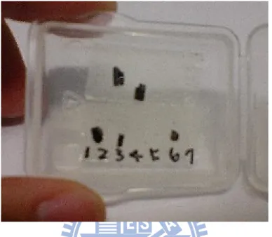
The fabrication of single crystals is very important for both fundamental researches and

industrial purposes. Figure 2-1 shows the hexagonal HoMnO3 single crystals used in this

study. The pure polycrystalline hexagonal HoMnO3 single crystals were synthesized by a

solid-state reaction of stoichiometric amount of Ho2O3 (99.99 %) and MnO2 (99.99 %). The

single crystals of hexagonal HoMnO3 have been grown via the high temperature flux method

[1-3] and in a floating zone furnace. The samples were synthesized for 15 hours at 1290 ℃, then annealed for 5 hours at 1150 ℃ in a platinum crucible and in an oxygen atmosphere.

After that, the temperature was decrease to room temperature with a rate of 1 ℃/h. The flux was decanted and well-shaped hexagonal platelike crystals with typical size of 2 × 3 × 0.25

mm3 were removed from the bottom of the crucible.

2.1.1 Orientation and structure of HoMnO

3

single crystals

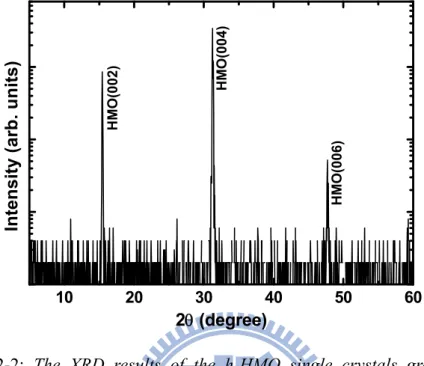
After growing the HoMnO3 single crystals, the most important thing is to characterize

their physical properties. Fig. 2-2 shows the X-ray diffraction (XRD) θ-2θ pattern (Cu Kα, λ = 1.5406 Å) for the h-HMO single crystals grew by the floating zone furnace method. The XRD

data evidently confirm the formation of the pure hexagonal HoMnO3 with the c-axis (space

group: P63cm) oriented normal to the largest crystal surface. The crystal structure of HoMnO3

has been shown in section 1.1 of chapter 1. The full width at half maximum (FWHM) ( 0.25°) of X-ray data indicates the good crystalline quality and grain alignment of the h-HMO

crystals. To further examine the in-plane texture of the crystals, we also measured the -scan

around the h-HMO reflection. The -scans display an evenly behaved six-fold symmetry,

Figure 2-1: The HoMnO3 single crystals used in this study. The largest surface

indicating that the in-plane grain alignment on the a-b plane well. The fitted lattice constant of

HoMnO3 single crystals for a- and c-axis were 6.142 Å and 11.408 Å, respectively [4-7].

The other useful parameters, e.g. lattice parameters, atomic positions, and discrepancy factors in Table. 2-1, from high-resolution neutron diffraction experiments were reported by A. Muñoz et al. [8].

Figure 2-2: The XRD results of the h-HMO single crystals grew by the

floating zone furnace method. The θ-2θ scans (plotted in semi-logarithmic scale) reveal that HMO crystals indeed hexagonal with c-axis orientation.

10 20 30 40 50 60 HM O (006 ) HM O (004 ) Int en s ity (arb . u n its) 2 (degree) HM O (00 2)

Table 2-1: The lattice constant, atomic positions, and discrepancy factors

2.1.2 Temperature–dependent susceptibility measurements

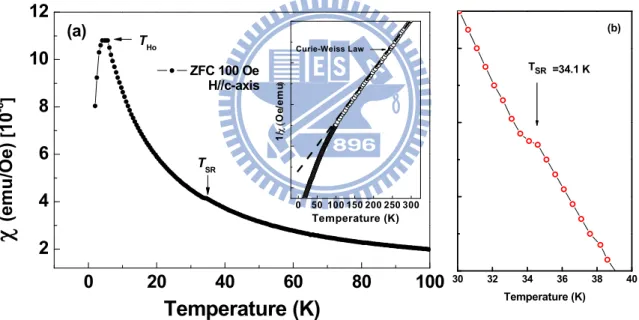
The magnetic properties were measured in a Quantum Design superconducting quantum interference device (SQUID) system. Fig. 2-3(a) and (b) show the characteristics of magnetization in the platelet samples examined by SQUID. The Mn-spin rotation transition

(TSR ~ 33 K) and the magnetic order of the Ho3+ ions (THO ~ 5 K) could be clearly observed in

the magnetization measurements (the arrows in Fig. 2.2(a) and the enlarge scale in Fig.

2-3(b)). However, the AFM transition of h-HoMnO3 is difficult recognized in magnetization

measurements due to the huge paramagnetic signal from rare-earth ion. These results consist with those reported by other researchers [9].

The AFM exchange coupling in a triangular lattice gives rise to spin frustration effects

and, at TN the Mn3+ moments order in a way so that neighboring Mn-moments form a 1200

angle [10]. In addition, most rare-earth ions carry their own magnetic moment oriented along

0 20 40 60 80 100 2 4 6 8 10 12 0 50 100 150 200 250 300 1/   Oe /e m u  Temperature (K) Curie-Weiss Law T_SR

Temperature (K)

ZFC 100 Oe H//c-axis T_Ho





(em u /O e) [ 10 -6 ] (a)

Figure 2-3: (a) The temperature-dependent susceptibility (χ(T)) of h-HMO

with a magnetic field of 100 Oe applied along c-axis. The inset shows the inverse susceptibility. The dashed line: the Curie-Weiss high temperature extrapolation. (b) To enlarge the figure in order to show the behavior of spin rotation.

30 32 34 36 38 40 Temperature (K)

T_SR =34.1 K (b)

the c-axis of the P63cm structure. The rare-earth moment can interact with the Mn3+ spins and

the dielectric polarization and thus increase the complexity of the phase diagram and the physical phenomena that can be observed. For example, the complex magnetic phase transition and different spin arrangements have been canvassed by the second harmonic generation or the neutron scattering measurements [8,11-12] which show two additional phase

transitions below TN indicating subtle changes in the magnetic order of the Mn3+ and Ho3+

ions at zero external magnetic field. At TSR ~ 33 K, a sharp Mn-spin reorientation transition

takes place at which all Mn-moments rotate in-plane with an angle of 900 and changes the

magnetic symmetry from P63cm (T > TSR) to P63cm (T < TSR) (illustrated in Fig. 2-4 [10]). At

lower temperatures, THo ~ 5 K, another change of the magnetic structure has been reported but

the magnetic order in this phase is still a matter of discussion. The transitions at TSR and THo

are accompanied by partial or complete magnetic ordering of the Ho3+ moments, but the detail

of the Ho-spin order has not been resolved yet. All magnetic transitions are well below the FE

Curie temperature of TC = 875 K.

Figure 2-4: The three Mn3+ spin configuration in hexagonal HoMnO3 [10].

The open circles indicate Mn ions at z=0, filled circles indicate Mn ions at z=c/2.

2.1.3 Transmittance spectrum

Fig. 2-5 shows the transmittance spectrum in the HoMnO3 single crystals which was

measured by a grating-type spectrophotometer (HITACHI high-technologies Corporation) in the photon energy range of 0.7-5.0 eV. According to the literatures [13-16], there are three

common features in the absorption spectrum of hexagonal ReMnO3 which performed by

Fourier-transform infrared spectrometer. First, the optical excitation causes the absorption

peak near ~ 1.7 eV at low temperature which is attributed to the charge transfer from e2g

orbitals (d and_xy d_x2_y2) to a1g orbitals (d_3z2_r2). Second, the relatively weak peak near ~ 2.2

eV comes from the charge transfer from e1g orbitals (d and_xz d ) to a_yz 1g orbitals (d_3z2_r2)

between the Mn 3d levels. Finally, a much stronger absorption peak at higher energy region

above 3 eV caused by the continuous charge transfer from O 2p to Mn 3d states as shown in

Fig. 2-5. In virtue of the transition metal Mn3+ ion sits at the center of a triangular bipyramid

Figure 2-5: The transmittance spectrum of hexagonal HoMnO3 single

crystals. The arrows show the three features. The inset shows the local environment MnO5 for photon energy above and below Edd.

1.0 1.5 2.0 2.5 3.0 3.5 4.0 4.5 5.0 0 10 20 30 40 50 60 70 80 90 > 3 eV 2.2 eV

Transmittance (%)

Photon Energy (eV)

h-HoMnO3

of five O2- ions at each corner, the d orbitals of the Mn3+ ion are split into three parts (e1g 、

e2g、a1g) due to the ligand field effects which arises mainly from the strong electrostatic

Coulomb repulsion of the negatively charged electrons in the oxygen orbitals (show in Fig. 2-6) [17-20].

The electric structures of h-HoMnO3 can be simulated by the first-principles

calculations since its structural parameters have been sufficiently studied. To deal with the

effects of strong Coulomb interactions among 3d electrons, one can use the local density

approximation (LDA) +U methods based on the density functional theory, as implemented in a linear combination of localized pseudo atomic orbital (LCPAO) code. Fig. 2-7 shows the

density of states for hexagonal YMnO3 calculated by Choi et al. [16].

2.2 Femtosecond time-resolved systems

In this section, we are going to introduce the optical systems used in this study which were built by ourselves. This measuring system has three parts which can be operated individually. The first part (subsection 2.2.1) is a pump-probe system. The second part (subsection 2.2.2) is a terahertz time-domain spectroscopy system. The final part (subsection 2.2.3) is a whole system combining the first and second parts, so-called optical pump terahertz probe system. In the following subsections in this dissertation will exhibit various systems respectively. In this section we only discuss the optical apparatus among these systems. On the contrary, the principles of operation will be discussed in chapter 3.

Figure 2-7: The orbital-resolved densities of states of Mn 3d orbitals and the

2.2.1 The polarized femtosecond pump-probe system

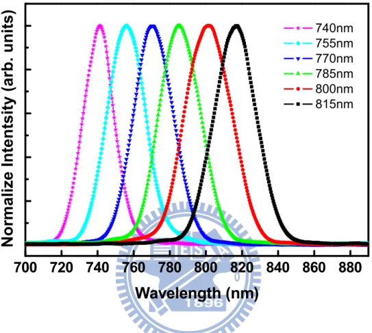
Figure 2-8 shows the details of the optical pump-probe system used in this study. The experiments were performed with a femtosecond Ti:sapphire laser pumped by an Nd:YAG laser with 532 nm. Fig. 2-9 shows the laser system which is a Ti:sapphire oscillator (Model: Micra-10) fabricated by “Coherent in USA”. The output laser is wavelength tunable from 815 nm to 740 nm via controlling the interval of the slit. The output spectrum can be measured by a spectrometer (Ocean optics, Model: USB4000-UV-VIS) as shown in Fig. 2-10. The spectral width of the output pulses was adjusted to ~25 nm (FWHM) for our measurements. Following, the output laser beam went through a beamsplitter (BS1) and was reflected 50 % of light as a pump beam (B1) used to generate the terahertz beam, whereas the remnant (B2) was transmitted and served as a probe which was used to probe the terahertz pulse. Moreover, the pump and probe beams used to do pump-probe experiments were taken from B2 and divided

Figure 2-8: The experimental setup for near-IR pump-probe spectroscopy.

Code : BS: beamsplitter, L: lens, A: acousto-optic modulator (AOM), M: mirror, WP: wave plate, P: polarizer, TS: time-delay stage, D: photodiode.

into B3 via a beamsplitter (BS2). The laser beam B3 passed through a prism pair in order to compensate the dispersion due to the optical components in the system. Both pump and probe beams passed through two acousto-optic modulators (AOM, A1-A2) respectively. However, only one in the pump beam was driven by the RF driver and modulated the pump beam at 1 MHz. After travelling through a delay stage (TS1), a half-wave (λ/2) plate (WP1-WP2), and a polarizer (P1-P2), the pump beam was focused by a 200-mm lens on the surface of a sample with ~ 200 μm in diameter. The λ/2 plate and polarizer allowed us to adjust the intensity and

polarization (electric field, E) of pump beam (both needed for intensity control). A mechanical

delay stage was used to vary the arrival time of pump pulses related to probe pulses at the position of samples. On the other hand, the probe beam only passed through the λ/2 plate and the polarizer after the AOM and focus on the surface of the sample with 150 μm in diameter by a 150-mm lens.

The powers of pump and probe beams were 50 mW and 2 mW, respectively. The best spatial overlap of pump and probe beams on the samples was realized by monitoring with a CCD

Figure 2-9: The Ti:sapphire laser cavity. The green line represents the

camera. The reflectivity changes of a probe beam were detected by using a photodiode detector and a lock-in amplifier [21-23].

2.2.2 The terahertz time-domain spectroscopy

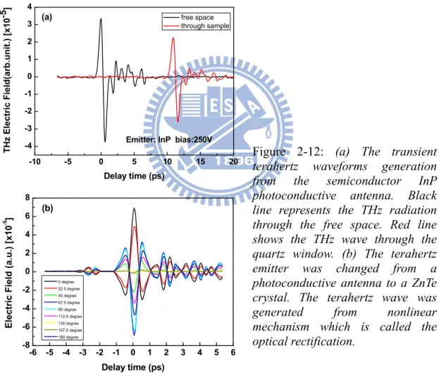
In past 20 years, the femtosecond excitation on photoconducting switches, unbiased and biased semiconductor surface, and strain layer heterostructures have been used to generate pulsed THz electromagnetic waves [24-29]. The THz waves can be collimated and transmitted over reasonable distances, and can be detected by using optically-gated photoconductive antennas. By adjusting the delay between the THz signal and the gating pulse, the amplitude and phase of the THz signals can be obtained.

Figure 2-10: The tunable wavelengths from 815 nm (1.52 eV) to 740 nm (1.68

eV) in the Ti:sapphire oscillator used in this study.

700 720 740 760 780 800 820 840 860 880

Norm

alize Intentsity (arb. units)

Wavelength (nm)

740nm 755nm 770nm 785nm 800nm 815nm

Figure 2-11 shows the optical setup of the THz time-domain system. In this system, the light source divided into two parts via beamsplitter (BS1), the first one was used to generate THz radiation (B1) called THz pump beam, and another was used to be the gating pulse called THz probe beam (B2). The optical pulses (B1) were normally incident to the terahertz emitter (TE) which was manufactured by low-temperature growth GaAs or InP. The THz pump beam was modulated by a mechanical chopper (CH1) operated at 1.3 kHz. The electric field of a terahertz pulse was sampled by scanning the delay (TS4) between the pump and probe pulses. A semiconductor GaAs photoconductive emitter was triggered by femtosecond laser pulses and radiated the THz pulses. The emitted THz pulses was collimated by two pairs of off-axis parabolical mirrors (PM1-PM4) and focused onto a nonlinear ZnTe electroptical crystal. A pellicle beamsplitter (PSP2) which is transparent for the terahertz beam was used to reflect

Figure 2-11: The experimental setup for the terahertz time-domain

spectroscopy. Code: BS: beamsplitter, L: lens, CH: chopper, M: mirror, TS: time-delay stage, TE: THz emitter, PM: parabolical mirror, WP: wave plate, PB: polarized beamsplitter, D: photodiode.

80% of the synchronized optical probe beam. The polarized THz wave and probe beam were collinearly aligned to a <110>-oriented ZnTe crystal. Then, we used a quarter-wave plate

(WP5) to add a /2 optical bias in the probe beam, which allows the system to operate in

the linear range. A Wollaston polarizer beamsplitter (PBS) was used to convert the terahertz-field-induced phase retardation of the probe beam into an intensity modulation between the two orthogonal linear-polarized beams. The optical intensity modulation was detected by using two balanced photodiodes (D3, D4) and a lock-in amplifier (SR830).

-6 -5 -4 -3 -2 -1 0 1 2 3 4 5 6 -8 -6 -4 -2 0 2 4 6 8 Ele c tr ic F ie ld (a .u .) [x1 0 -5 ] Delay time (ps) 0 degree 22.5 degree 45 degree 67.5 degree 90 degree 112.5 degree 135 degree 157.5 degree 180 degree (b) -10 -5 0 5 10 15 20 -4 -3 -2 -1 0 1 2 3 4 THz Elect ric Field( ar b .unit .) [ x10 -5] Delay time (ps) free space through sample

Emitter: InP bias:250V

(a)

Figure 2-12: (a) The transient

terahertz waveforms generation from the semiconductor InP photoconductive antenna. Black line represents the THz radiation through the free space. Red line shows the THz wave through the quartz window. (b) The terahertz emitter was changed from a photoconductive antenna to a ZnTe crystal. The terahertz wave was generated from nonlinear mechanism which is called the optical rectification.

2.2.3 The optical pump-terahertz probe system setup

The optical pump-THz probe system was performed by combined the optical pump-probe system and THz time domain system. In order to generate THz by nonlinear effect, we change the laser source from the Ti:sapphire oscillator to amplifier (Model: Coherent, Legend). The high peak power of Ti:sapphire femtosecond amplifier allows for the nonlinear optical conversion of the fundamental wavelength of 800 nm to the wavelengths of ultraviolet or infrared (THz). In fact, the combination of an optical pump with THz probe has been used to investigate the relaxation dynamics of photoexcited carriers in a lot of materials, such as superconductors [30], semiconductors [31-34], dielectrics [35], and liquids [36-37]. A diagram of the optical pump-THz probe experimental setup is shown in Fig. 2-13. The primary light source is a Ti:sapphire regenerative amplifier, which typically produces sub-100 fs (FWHM) and 800 nm pulses at a 5 kHz repetition rate. The pulses from amplifier laser pass through all kinds of optical components as mentioned in above subsections. It should be

emphasized some differences between pump-probe system and THz time domain system. One is the amplifier laser pulses without the dispersion compensation because the low frequency modulation by a mechanical chopper (CH2) instead of an AMO. Another one is the generation of THz radiation from an emitter (TE) of a ZnTe crystal instead of a semiconductor antenna in order to get higher power THz radiation.

The Fig. 2-14 shows the concepts of optical pump-THz probe measurements. The black circles represent the arrival time of a pump pulse at the sample surface. The curve shown in Fig. 2-14 represents the reflectivity changes induced by a pump pulse as increasing the delay time. We can measure the THz waveform with changing the delay time of a pump pulse. Thus, the variation of the dielectric function after pump excitation can be obtained. In general, we can obtain the transient information about the carrier dynamics induced by pump laser. The time-resolved transient dielectric function allows someone to know the behavior of electrons

Delay time position1 _position2 position3 position X -8 -6 -4 -2 0 2 4 6 8 -0.00006 -0.00004 -0.00002 0.00000 0.00002 0.00004 Pump Power:140nW A m plit ude ( a. u. ) Delay Time(PS) THz Emitter :InP DC bias:200V -8 -6 -4 -2 0 2 4 6 8 -0.00006 -0.00004 -0.00002 0.00000 0.00002 0.00004 Pump Power:140nW A m p lit ude ( a. u. ) Delay Time(PS) THz Emitter :InP DC bias:200V -8 -6 -4 -2 0 2 4 6 8 -0.00006 -0.00004 -0.00002 0.00000 0.00002 0.00004 Pump Power:140nW A m pl itude ( a. u. ) Delay Time(PS) THz Emitter :InP DC bias:200V -8 -6 -4 -2 0 2 4 6 8 -0.00006 -0.00004 -0.00002 0.00000 0.00002 0.00004 Pump Power:140nW A m plit ud e ( a.u .) Delay Time(PS) THz Emitter :InP DC bias:200V

or lattice in one material. Fig. 2-15 shows an example, the results of optical pump-THz probe experiments in semiconductor InP. The peak amplitude of THz pulses plotted as a function of delay time of pump pulses. The excitation of pump laser causes the changes of refractive index and thus causes the changes in THz transmittance [38-41].

-50 0 50 100 150 200 250 300 350 400 -10.5 -9.0 -7.5 -6.0 -4.5 -3.0 -1.5 0.0 1.5 Ampl itude of THz peak (V) [x10 -6 ]

Pump beam delay (ps)

1 mW 1.5 mW 2 mW 2.5 mW

Figure 2-15: The peak amplitude of THz radiation as a function of the delay

Figure 2-16 shows the experimental setup. The experimental apparatus includes the optical cryostat for measuring temperature-dependent optical spectra.

Figure 2-16: The experimental apparatus including the optical cryostat for

References

[1] B. Lorenz, F. Yen, M. M. Gospodinov, and C. W. Chu, Phys. Rev. B 71, 014438 (2005). [2] E. Galstyan, B. Lorenz, K. S. Martirosyan, F. Yen, Y. Y. Sun, M. M. Gospodinov, and C. W.

Chu, J. Phys.: Condens. Matter 20, 325241 (2008).

[3] A. P. Litvinchuk, M. N. Iliev, V. N. Popov, and M. M. Gospodinov, J. Phys.: Condens. Matter 16, 809 (2004).

[4] P. Murugavel, J.-H. Lee, D. Lee, T. W. Noh, Younghun Jo, Myung-Hwa Jung, Yoon Seok Oh, and Kee Hoon Kim, Appl. Phys. Lett. 90, 142902 (2007).

[5] J.-W. Kim, K. Nenkov, L. Schultz, and K. Dörr, J. Magn. Magn. Mater. 321, 1727 (2009). [6] J.-W. Kim, L. Schultz, K. Dörr, B. B. Van Aken, and M. Fiebig, Appl. Phys. Lett. 90,

012502 (2007).

[7] N. N. Loshkareva, A. S. Moskvin, and A. M. Balbashov, Physics of the Solid State 51, 930 (2009).

[8] A. Muñoz, J. A. Alonso, M. J. Martínez-Lope, M. T. Casáis, J. L. Martínez, and M. T. Fernández-Díaz, Chem. Mater. 13, 1497 (2001).

[9] B. Lorenz, A. P. Litvinchuk, M. M. Gospodinov, and C. W. Chu, Phys. Rev. Lett. 92, 087204 (2004).

[10] O. P. Vajk, M. Kenzelmann, J. W. Lynn, S. B. Kim, and S.-W. Cheong, J. Appl. Phys. 99, 08E301 (2006).

[11] M. Fiebig, D. Fröhlich, T. Lottermoser, and K. Kohn, Appl. Phys. Lett. 77, 4401 (2000). [12] M. Fiebig, D. Fröhlich, T. Lottermoser, and M. Maat, Phys. Rev. B 66, 144102 (2002). [13] A. B. Souchkov, J. R. Simpson, M. Quijada, H. Ishibashi , N. Hur, J. S. Ahn, S. W.

Cheong, A. J. Millis, and H. D. Drew, Phys. Rev. Lett. 91, 027203 (2003).

[14] R. C. Rai, J. Cao, J. L. Musfeldt, S. B. Kim, S.-W. Cheong, and X. Wei, Phys. Rev. B 75, 184414 (2007).

[15] Woo Seok Choi, Soon Jae Moon, Sung Seok A. Seo, Daesu Lee, Jung Hyuk Lee, Pattukkannu Murugavel, Tae Won Noh, and Yun Sang Lee, Phys. Rev. B 78, 054440 (2008).

[16] Woo Seok Choi, Dong Geun Kim, Sung Seok A. Seo, Soon Jae Moon, Daesu Lee, Jung Hyuk Lee, Ho Sik Lee, Deok-Yong Cho, Yun Sang Lee, Pattukkannu Murugavel, Jaejun Yu, and Tae W. Noh, Phys. Rev. B 77, 045137 (2008).

[17] Deok-Yong Cho, S.-J. Oh, Dong Geun Kim, A. Tanaka, and J.-H. Park, Phys. Rev. B 79, 035116 (2009).

[18] H. C. Shih, T. H. Lin, C. W. Luo, K. H. Wu, J.-Y. Lin, J. Y. Juang, T. M. Uen, J. M. Lee, J. M. Chen, and T. Kobayashi, Phys. Rev. B 80, 024427 (2009).

[19] C.-Y. Ren, Phys. Rev. B 79, 125113 (2009).

[20] C. Degenhardt, M. Fiebig, D. Fröhlich, Th. Lottermoser, and R. V. Pisarev, Appl. Phys. B

73, 139 (2001).

[21] C. W. Luo, “Anisotropic Ultrafast Dynamics in YBa2Cu3O7-δ Probed by Polarized

Femtosecond Spectroscopy,” Doctoral thesis, National Chiao Tung University, Taiwan, (2003).

[22] J.-C. Diels, and W. Rudolph, “Ultrashort Laser Pulse Phenomena”, Academic Press (1996).

[23] J. Shah, M. Cardona, P. Fulde, K. V. Klitzing, and H. J. Queisser, “Ultrafast spectroscopy of semiconductors and semiconductor nanostructures”, second enlarger edition, Springer, (1996).

[24] D. H. Auston and M. C. Nuss, IEEE J. QE-24, 184 (1988).

[25] X.-C. Zhang, X. F. Ma, Y. Jin, T. –M. Lu, E. P. Boden, P. D. Phelps, K. R. Stewart, and C. P. Yakymyshen, Appl. Phys. Lett. 61, 3080 (1993).

[27] X.-C. Zhang, B. B. Hu, J. T. Darrow, and D. H. Auston, Appl. Phys. Lett. 56, 1011 (1990).

[28] B. B. Hu, J. T. Darrow, X.-C. Zhang, D. H. Auston, and P. R. Smith, Appl. Phys. Lett. 56, 886 (1990).

[29] X.-C. Zhang, B. B. Hu, S. H. Xin, and D. H. Auston, Appl. Phys. Lett. 57, 753 (1990). [30] H. Wals, P. Seidel, and M. Tonouchi, Physica C 367, 308 (2002).

[31] H. K. Nienhuys, and Villy sundstrom, Appl. Phys. Lett. 87, 012101 (2005). [32] J. Zielbauer, and M. Wegener, Appl. Phys. Lett. 68, 1223 (1996).

[33] G. Segschneider, F. Jacob, T. Loffler, H. G. Roskos, S. Tautz, P. Kiesel, and G. Dohler, Phys. Rev. B 65, 125205 (2002).

[34] K. P. H. Lui, and F. A. Hegmann, J. Appl. Phys. 93, 9012 (2003).

[35] J. Shan, F. Wang, E. Knoesel, M. Bonn, and T. F. Heinz, Phys. Rev. Lett. 90, 247401 (2003).

[36] E. Knoesel, M. Bonn, J. Shan, and T. F. Heinz, Phys. Rev. Lett. 86, 340 (2001). [37] E. Knoesel, M. Bonn, J. Shan, and T. F. Heinz, J. Chem. Phys. 121, 394 (2004).

[38] H. F. Tiedje, H. K. Haugen, and J. S. Preston, Optics Communication 274, 187 (2007). [39] D. G. Cooke, A. N. MacDonald, A. Hryciw, A. Meldrum, J. Wang, Q. Li, and F. A.

Hegmann, J. Mater. Sci.: Mater. Electron. 18, 447(2007).

[40] J. E. Pedersen, V. G. Lyssenko, J. M. Hvam, P. Uhd Jepsen, S. R. Keiding, C. B. Sørensen, and P. E. Lindelof, Appl. Phys. Lett. 62, 1265 (1993).

Chapter 3

The femtosecond pump-probe spectroscopy

Time-resolved spectroscopy is a very important and direct tool for investigating the dynamics problems. Many physical phenomena were revealed via the ultrafast pump-probe method. In previous chapter 2, we have described the characteristics of samples and the measurement systems. In this chapter, we are going to introduce the fundamental principle of pump-probe technique. First, we discuss the characteristics of femtosecond pulse laser. Next, we discuss the principle of time-resolved pump-probe spectroscopy. Finally, we focus on the physical origins of the coherent spike signals induced by two laser beam interference.

3.1 The characteristic of femtosecond pulse laser

Up to now, there are many techniques for generating the short laser pulse, such as Q-switch [1-4], active mode-locking [5-10], passive mode-locking, the hybrid mode-locking [11-12], and the self-mode-locking [13-14]. The pulse duration generated by above methods varies from nanosecond to femtosecond. In this section, we will only talk about the characteristics of the femtosecond laser pulses which was generated via self-mode-locking

method.

3.1.1 The light pulses

The plane waves are the simplest propagation solutions which are solved via the Maxwell’s equations: Re( ( )) 0 i t kr y E e E   _,    _ 2  c k (3.1)

This particular solution (3.1) describes the propagation of a transverse electric field E _y

along the propagation axis at any given point x. When the monochromatic plane wave at the

origin (x0), a rewriting of Eq. (3.1) is as follows, (shown in Fig. 3.1 (a))

Re( 0 ) 0 t i y E e E   (3.2)

The time representation of the field is an unlimited cosine function. A light pulse can be constructed by multiplying Eq. (3.2) with a bell-shaped function. In general case, one can use a Gaussian function to produce a light pluse,

Re( ( )) 0 0 2 _{i t} t y E e E    (3.3)

and its time evolution is shown in Fig. 3.2 (a). In Eq. (3.3),  is the shape factor of the

Gaussian envelope; it is proportional to the inverse of the squared duration t , i.e. ₀ 2

0 

  t .

There are three examples (0.5, 1.2, 4) shown in Fig. 3.2 (a). Moreover, the spectral of a

light pulse can be obtained by the Fourier transform of the time evolution function of a pulse.

Fig. 3-1(b) shows the result of a plane wave with the unique angular frequency ₀ and its

Fourier transform is a delta function (₀). The Fourier transform of Gaussian pulse is also

a Gaussian function (shown in Fig. 3-2 (b)). Thus, a light pulse must be constructed by many frequencies which are more than that of a plane wave. The numerical expression for the

Figure 3-1: (a) Schematic time evolution

of the electric field of a monochromatic plane wave. (b) The numerical Fourier transform of the cosine function. As the width of the cosine function grows larger and larger, the spectrum in frequency domain becomes a delta function with zero width.

Figure 3-2: (a) Time evolution of the

electric field with a Gaussian-shaped pulse. This pulse is constructed by multiplying a cosine function with a Gaussian envelope function. (b) The numerical Fourier transform of the Gaussian function. The spectrum in frequency domain is also a Gaussian function with a width which is proportional to  -1.0 -0.5 0.0 0.5 1.0 Time (a) -1.0 -0.5 0.0 0.5 1.0 _{}   Time (a) A rb. un it s angular frequency  ₀ (b) delta-function (₀₎ =0.5 =1.2 =4 A rb. un its ₀ angular frequency  (b) E()=exp[-(_)2/4] Gaussian function

F.F.T. F.F.T.

spectrum is given in Fig. 3-2 (b) and the width of the spectrum is proportional to  . In other words, if the signal of Gaussian pulse in time domain is narrower, its Fourier transform spectrum is broader [15-16].

3.1.2 Method for the generation of ultrafast laser pulses

The self-mode-locking is the most popular method to generate the ultrashort laser pulses with duration as short as a few femtoseconds. The Kerr-lens mode-locking (KLM) is a method of mode-locking lasers via a nonlinear optical process known as the optical Kerr effect (self-mode-locked Ti:sapphire laser using the KLM shown in Fig. 3-3). The nonlinear properties of the amplifying medium are always very important for the locking process. The optical Kerr effect is a process which results from the nonlinear response of an optical medium to the electric field of an electromagnetic wave. The refractive index of the medium is dependent on the field strength.

Figure 3-3: The typical cavity design of a self-mode-locked Ti:sapphire

Because of the non-uniform power density distribution in a Gaussian beam (shown in Fig. 3-4), the refractive index changes across the beam profile; the refractive index experienced by the beam is greater in the centre of the beam. The fact that the amplifying medium is

nonlinear implies that its refractive index is a function of the intensity: nn₀ n₂I. The

Gaussian wave therefore does not feel a homogeneous refractive index as it passes through the medium.

Therefore, the amplifying medium behaves like a converging lens and focuses the beam just like a lens (Kerr lens). Following, the intensity–differentiated self-focusing associated with the natural cavity losses plays a part similar to that of the saturable absorber in the passive mode-locking method, indeed, self-mode-locking of the modes arises. A slit can be placed inside the cavity to help the self-locking process since it increases the difference between the losses undergone by the weak intensities and those undergone by the intensity maxima. Fig. 3-5 illustrates the evolution from a continuous regime to a mode-locked regime. Moreover, if one wants to start the pulsed process, one can insert a rapidly rotating optical slide

Aperture

cw 

pulse 

Intentsity 

Kerr   medium