六邊形離心調速器的旋轉機械之渾沌控制及渾沌同步

全文

(1)國立交通大學機械工程研究所博士論文. 六邊形離心調速器的旋轉機械之渾沌控制及渾沌同步 Chaos Control and Chaos Synchronization for a Rotational Machine with a Hexagonal Centrifugal Governor. 研究生：李青一指導教授：戈正銘. 教授. 中華民國九十三年六月.

(2) 六邊形離心調速器的旋轉機械之渾沌控制及渾沌同步研究生：李青一. 指導教授：戈正銘教授. 國立交通大學機械工程研究所. 摘要本篇論文研究一帶六邊形調速器之旋轉機械的渾沌動力行為，自治、非自治及時滯系統均予以討論。由李亞普諾夫直接法可求得自治系統平衡點的穩定條件。應用一些數值分析，如相圖、功率譜法、龐加萊映射法、及李亞普諾夫指數可觀察到週期解與渾沌運動。參數變化對系統的影響可以由分歧圖及參數圖表現出來。除此之外，利用一些控制方法來有效地控制渾沌現象。最後，對於系統的渾沌反控制與渾沌同步，也提供了控制器設計的一些方法。. i.

(3) Chaos Control and Chaos Synchronization for a Rotational Machine with a Hexagonal Centrifugal Governor Student：Ching-I Lee. Advisor：Zheng-Ming Ge. Institute of Mechanical Engineering National Chiao Tung University. ABSTRACT The chaotic dynamics of the rotational machine with a hexagonal centrifugal governor are studied in this thesis. Autonomous, nonautonomous and time-delay systems are discussed. The Lyapunov direct method is applied to obtain conditions of stability of the equilibrium points of autonomous system. By applying numerical results, phase diagrams, power spectrum, Poincaré maps, and Lyapunov exponents are presented to observe periodic and chaotic motions. The effect of the parameter changes in the system can be found in the bifurcation and parametric diagrams. Besides, several methods are used to control chaos effectively. Finally, some different procedures for the design of the controller are proposed for anticontrol and synchronization of chaos of the governor system.. ii.

(4) 誌. 謝. 本論文得以完成，首先要感謝恩師. 戈正銘教授多年來的悉心指導。. 老師除了卓越的專業學識以外，其嚴謹的治學態度及追求新知的研究熱誠都是學生在學習旅程上永遠的標竿。論文口試期間，承蒙董必正教授、張家歐教授、周傳心教授與邵錦昌教授等諸位審查委員，對本論文提供了許多的寶貴意見，使本論文更臻完善。特此僅致誠摯的謝意。此外，論文研究期間，承蒙許多學長與學弟對我的協助與鼓勵，亦銘感在心。漫長的求學過程中，要感謝愛妻瑛瓔這一路任勞任怨的付出與扶持，也要感謝父母親的支持與鼓勵。最後再一次向恩師戈正銘教授致上最深之謝意。. iii.

(5) CONTENTS CHINESE ABSTRACT …………….………………………………………………. i ABSTRACT ………………………………………………………………………….ii ACKNOWLEDGMENTS …………………………………………………………..iii CONTENTS………………………………………………………………………….iv LIST OF FIGURES………………………………………………….………………vi Chapter 1. Introduction ………………………………………………………… 1. Chapter 2. The Analytical Analysis of the System……………………………... 5. 2.1. Equations of Motion …………………………………………………..5. 2.2. Stability Analysis by Lyapunov Direct Method ……………………… 7. Chapter 3. Chaotic Dynamics of the System………………………………….. 12. 3.1 Chaos, Controlling Chaos and Synchronization of Chaos of Autonomous System…………………………………………………. 12 3.1.1. Phase Portraits , Poincaré Map and Power Spectrum ……………12. 3.1.2 Lyapunov Exponent and Lyapunov Dimension …………………14 3.1.3. Controlling Chaos ………………………………………………..15. 3.1.4. Chaos Synchronization and Phase Synchronization……………..19. 3.2 Anticontrol. and. Synchronization. of. Chaos. of. Autonomous. System………………………………………………………………...22 3.2.1 Adding a Linear Feedback…………………….………………… 22 3.2.2. Adding a Nonlinear Feedback ………………………………….23. 3.2.3 Chaos Synchronization …………………………………………..23 3.3 Chaos, Control, Anticontrol and Synchronization of Chaos for the System with Time-Delay …………………………………………… 29 iv.

(6) 3.3.1. Regular and Chaotic Dynamics of Time-Delay System …………29. 3.3.2. Controlling Chaos ………………………………………………..30. 3.3.3 Chaos Synchronization …………………………………………..32 3.3.4. Anticontrol of Chaos …………………………………………...35. 3.4 Chaos, Controlling Chaos and Synchronization of Chaos of Nonautonomous System …………………………………………….. 36 3.4.1. Regular and Chaotic Dynamics of Nonautonomous System …….36. 3.4.2. Controlling Chaos ………………………………………………..40. 3.4.3 Chaos Synchronization …………………………………………..46 Chapter 4. Conclusions……………………….………………………………… 48. REFERENCES ……………………………………………………………………. 51. v.

(7) LIST OF FIGURES Fig. 2.1. Physical model of the system……………………………………………...53 Fig. 3.1. (a) Phase portrait and Poincaré map for q=2.3 (b) q=3 (c) phase portrait for q=5.5 (d) Poincaré map for q=5.5…………………………………………54 Fig. 3.2 (a) Power spectrum for q=2.3 (b) q=5.5…………………………………...55 Fig. 3.3. The Lyapunov exponents for q between 2.3 and 5.5………………………56 Fig. 3.4. Phase portrait of controlled system (a) τ = 5 , (b) τ = 4 ………………...57. Fig. 3.5. Phase portrait of controlled system via adaptive feedback control………..57 Fig. 3.6. Phase portrait of controlled system via linear feedback control…………..58 Fig. 3.7. Phase portrait of controlled system via optimal control…………………..58 Fig. 3.8 Chaos synchronization via a linear feedback approach……………………59 Fig. 3.9. Chaos synchronization via adaptive feedback with k1=10 and k2=1………60 Fig. 3.10. The projection of the attractor in the x-y plane(a) and x-z plane(b) with the coupling strength K = 0.1 ………………………………………………...61 Fig. 3.11. (a) shows the maximum absolute difference of two phases. (b) shows the maximum absolute difference of two trajectories. (c) The cross-correlation function ξ (0) with τ = 0 ……………………………………………….62 Fig. 3.12. The Lyapunov exponents of coupled system……………………………...63 Fig. 3.13. Phase portrait of uncontrolled system ( a1 = a 2 = a3 = 0)………………..64 Fig. 3.14. Phase portrait of controlled system with a1 = 0.2, a 2 = −0.1, a3 = −0.1 …65 Fig. 3.15. parameter diagram of (a) a 2 versus a3 for a1 = 0.2 , (b) a 2 versus a1 for a3 = −0.1 ……………………………………………………………...66 Fig. 3.16. Phase portrait of controlled system with ε = 0.01 ……………………….67 Fig. 3.17. Chaos synchronization via a linear feedback with k1 = 0.2 ……………...68 Fig. 3.18. Chaos synchronization via a nonlinear feedback with k 2 = 0.2 …………69 vi.

(8) Fig. 3.19. Chaos synchronization via adaptive feedback with k3=0.5 and k4=0.2…...70 Fig. 3.20. Chaos synchronization via backstepping design…………………………. 71 Fig. 3.21. The minimum value of U with respect to the coupling constant k1 . ……..72 Fig. 3.22. The difference U versus the parameter q for k1 = 0.2 .…………………...72 Fig. 3.23. Time evolution of the parameter q by the random optimization process.…73 Fig. 3.24. A mass-spring system.……………………………………………………..74 Fig. 3.25. (a) Phase portrait for q=3 (b) q=5.5. ………………………………………74 Fig. 3.26. (a) Time history ,(b) power spectrum for q=5.5 . ………………………..75 Fig. 3.27. Controlled system via adaptive feedback.…………………………………76 Fig. 3.28. (a)Phase portrait of controlled system via linear feedback control for K2 = 0.5, (b) K2 = 5.…………………………………………………………...76 Fig. 3.29. Chaos synchronization via a unidirectional linear feedback approach for K=3.………………………………………………………………………..77 Fig. 3.30. Chaos synchronization via a mutual linear feedback approach for K=1.5. .78 Fig. 3.31. Chaos synchronization via a mutual linear feedback approach for K=3. …79 Fig. 3.32. Chaos synchronization via a mutual nonlinear feedback approach for K=1.5. ………………..…………………………………………………………..80 Fig. 3.33. The maximum absolute difference of mean frequency between two chaotic subsystems.………………………………………………………………...81 Fig. 3.34. (a) A sawtooth function, (b) Phase portrait of controlled system.…………82 Fig. 3.35. (a) Phase portrait and Poincaré map for q=2.07 (b) q=2.14 (c) phase portrait for q=2.21 (d) Poincaré map for q=2.21.…………………………………..83 Fig. 3.36. (a) Power spectrum for q=2.07 (b) q=2.21. ……………………………….84 Fig. 3.37. Bifurcation diagram of q versus x.………………………………………...85 Fig. 3.38. (a) Parametric diagram of q versus b (b) q versus ω . ……………………86 Fig. 3.39. The largest Lyapunov exponent for q between 2.07 and 2.21. ……………87 vii.

(9) Fig. 3.40. Bifurcation diagram of T versus x.………………………………………...88 Fig. 3.41. Bifurcation diagram of v versus x. ………………………………………...88 Fig. 3.42. Bifurcation diagram of ρ versus x. ……………………………………...89 Fig. 3.43. Bifurcation diagram of K versus x. ………………………………………..89 Fig. 3.44. (a) Parameter converge to q=2.07 from chaotic motion q=2.21 (b) Phase portrait and Poincaré map of controlled system. ………………………….90 Fig. 3.45. (a) Parameter converge to q=2.14 from chaotic motion q=2.21 (b) Phase portrait and Poincaré map of controlled system.…………………………..91 Fig. 3.46. (a) Phase portrait and Poincaré map of controlled system (b) the error signal. ……………………………………………………………………………92 Fig. 3.47. Bifurcation diagram of K 1 versus x. ……………………………………..93 Fig. 3.48. Bifurcation diagram of K 2 versus x.……………………………………..94 Fig. 3.49. Chaos synchronization via linear feedback with k =0.2. ………………….95. viii.

(10) Chapter 1 Introduction During the past one and half decades, a large number of studies have shown that chaotic phenomena are observed in many physical systems that possess non-linearity. It was also reported that the chaotic motion occurred in many nonlinear control system [1-4]. In nature, most of physical systems are nonlinear and can be described by the nonlinear equations of motion. If the nonlinear term can be ignored, it is possible to linearize and easily solve it by the already known methods. The linearization process is reasonable, whereas for some nonlinear systems the simplification is inadequate and inaccure. Hence the researches of nonlinear systems spread quickly today. For the nonlinear system, the study of the types of periodic solutions, the effects to the solutions caused by different parameters and initial conditions, the stability analysis of the solutions, consist of the major tasks. Besides, a substantial understanding of the complicated phenomena arised from nonlinearity is also what we are interested in. The central characteristics are that a process like randomization happens in the deterministic system and small differences in the initial conditions produce very great ones in the final phenomena. The irregular and unpredictable motions of many nonlinear systems have been labeled 'chaotic'. In the end of nineteen century Poncaré first pointed out some important concepts of chaos theory like homoclinic, bifurcation, ...etc. Lorenz researched the strange. 1.

(11) changes in the atmosphere which is the first example to study chaos in 1963. A large number of studies on the chaotic behavior have been reached up to now. A characteristic property of chaotic dynamics is the sensitive dependence on initial condition. Different initial conditions may cause entirely different trajectories for the system. However, Pecora and Carroll [5] showed that synchronization can be achieved for the chaotic systems. This interest phenomenon plays a significant role in the chaotic dynamics of communication signals and may be applied to the real-time recovery of signals that have been masked in a strange attractor and thus to encode communication. Other applications of synchronization of chaos also have expectative potential [6-10]. Sometimes, chaos is not only useful but actually important. For example, chaos is desirable in many applications of liquid mixing while the required energy is minimized. For this purpose, making a non-chaotic dynamical system chaotic is called “anticontrol of chaos”. This implies that the regular behaviors will be destroyed and replaced by chaotic behavior. In the real world, chaotic behavior is important. Examples include liquid mixing, humam heartbeat regulations, resonance prevention in mechanical systems and secure communication[11]. In previous researches, most of them are concentrated to several well-known systems, such as Lorenz system, Rössler system and Chua’s circuits system, etc. In this thesis, an autonomous hexagonal centrifugal governor system is studied. The centrifugal governor is a device that automatically controls the speed of an engine and prevents the damage caused by sudden change of load torque. It plays an important role in many rotational machines such as diesel engine, steam engine and so on. When an engine. 2.

(12) system is subjected to external disturbances, the speed of the engine will vary. In order to diminish the change of engine speed, and avoid the chaotic motion emerging in the operational process of the engine, in this thesis the regular and chaotic dynamics of a rotational machine with centrifugal governor is studied in detail. Furthermore, controlling chaos, synchronization and anticontrol of chaos of the governor system are also studied. A lot of modern techniques are used in analyzing the deterministic nonlinear system behavior. Both analytical and computational methods are employed to obtain the characteristics of the nonlinear systems. In Chapter 2, the governing equations of motion will be formulated then the stability of the fixed points of the autonomous system are studied by the Lyapunov direct method. In Chapter 3, many numerical techniques are studied for analyzing the nonlinear system behavior. A variety of the periodic solutions and the phenomena of the chaotic motion can be presented in the phase diagrams, Poincaré maps and power spectrum. The effect of the parameters changed in the system can be found in the bifurcation and parametric diagrams. Further, chaotic motion can be detected by using Lyapunov exponents and Lyapunov dimensions. In order to improve the performance of a dynamic system or to avoid the chaotic phenomena, we must control a chaotic motion to a periodic motion that is beneficial for working with a particular condition. It is thus of great practical importance to develop suitable control methods. Recently much interest has been focused on this type of problem - controlling chaos[4,6,12]. For this purpose, one uses various methods for controlling chaos. The addition of constant motor torque, the addition of periodic torque, using periodic impulse input as a control torque, the delayed feedback control, external force 3.

(13) feedback control, Bang-Bang control, optimal control and adaptive control are used to control chaos. Finally, attention is shifted to the synchronization and anticontrol of chaos. For synchronization of chaos, the chaotic system is decomposed into two subsystems proposed by Pecora and Carroll[5]. In the thesis, linear feedback, nonlinear feedback, adaptive feedback, backstepping design and parameter evaluation from time sequences approaches are discussed for synchronization of two coupled chaotic system, respectively. For anticontrol of chaos, two different procedure, linear and nonlinear controllers with certain feedback gain are proposed to anticontrol, i.e. to chaotify, the governor system.. 4.

(14) Chapter 3 Chaotic Dynamics of the System 3.1 Chaos, Controlling Chaos and Synchronization of Chaos of Autonomous System In nonlinear dynamical systems, variation of system parameters may cause sudden change in the qualitative behavior of their state. The state change is referred to as a bifurcation and the parameter value at which the bifurcation occurs is called the bifurcation value. Denoting φ = x, φ& = y, ω = z, equation (2.1.4) is rewritten in the form x& = y. 1 y& = dz 2 cos x + (e + pz 2 ) sin 2 x − sin x − by 2 z& = q cos x − F. (3.1.1). The condition for the eigenvalues of Jacobian consisting of a pure imaginary pair and eigenvalue with negative real part can be shown to be qc = 2.2558. Here q is considered as the control parameter to be varied for the occurrence of Hopf bifurcation. qc is the critical value when the values of parameters d , e, p, F , b are given as 0.08, 0.8, 0.04, 1.942, 0.4, respectively.. 3.1.1 Phase Portraits , Poincaré Map and Power Spectrum The phase portrait is the evolution of a set of trajectories emanating from various initial conditions in the state space. When the solution reaches steady state, the transient behavior disappears. The idea of transforming the 12.

(15) study of continuous systems into the study of an associated discrete system was presented by Henri Poincaré. One of many advantages of Poincaré map is to reduce dimensions of the dynamical system. The solution of period-1T in the phase plane will become one point in the Poincaré map. Usually, the period of the trajectories is not explicitly known for the autonomous system, so the choice of the Poincaré section is differ from the nonautonomous system. The Poincaré section of the three-dimensional autonomous system Eq. (3.1.1) is defined by Σ = {( x, y , z ) ∈ R × R × R z = z 0 }. and satisfies the condition n ⋅ ( x − x∑ ) > 0. The vector n normal to Σ is given by ⎡ 0⎤ n = ⎢ 0⎥ ⎢ ⎥ ⎣⎢1⎦⎥. and xΣ is point located on the section Σ . As q is increased passing through the critical value 2.2558, the supercritical hopf bifurcation occurs, i.e., a stable fixed point becomes unstable and a stable limit cycle appears. Then a cascade of period-doubling bifurcations develops which leads the system into chaos. By using fourth order Runge-Kutta numerical integration method, the phase plane and Poincaré map of the system, equation (3.1.1), is plotted in Fig. 3.1(a), (b) for q = 2.3, 3, respectively. Clearly, the motion is periodic. But Fig. 3.1(c), (d) for q = 5.5 show the chaotic states. Because the Poincaré map is neither a finite set of points nor a closed orbit, the motion may be chaotic. A valuable technique for the identification and characterization of the system is the power spectrum. This representation is useful for dynamical 13.

(16) analysis. The periodic motion of autonomous system are observed by the portraits of power spectrum in Fig. 3.2(a) for q = 2.3. The solution of system is period-1T, and the power spectrum exhibits a strong peak at the principal frequency Apparently, the spectrum of the periodic motion only consists of discrete frequencies. As q = 5.5 chaos occurs, the spectrum is a continuous broad-band one shown in Fig. 3.2(b). The noise-like spectrum is the characteristic of chaotic dynamical system. Although a broad spectrum does not guarantee sensitivity to initial conditions, it is still a reliable indicator of the chaos.. 3.1.2 Lyapunov Exponent and Lyapunov Dimension The Lyapunov exponent may be used to measure the sensitive dependence upon initial conditions. It is an index for chaotic behavior. Different solutions of dynamical system, such as fixed points, periodic motions, quasiperiodic motion, and chaotic motion can be distinguished by it. In three dimensional space, the Lyapunov exponents for a strange attractor, a limit cycle and a fixed point are described by (+,0,－), (0,－,－) and (－,－,－), respectively[15]. As q = 2, three Lyapunov exponents are obtained, respectively; λ1 = −0.0526, λ2 = −0.0535, λ3 = −0.2939 , which the motion converges to fixed. point. For q = 2.3 and q = 5.5, the Lyapunov exponents are λ1 = 0, λ2 = −0.1951, λ3 = −0.205 and λ1 = 0.0839, λ2 = 0, λ3 = −0.484 , respectively.. The Lyapunov exponents of the solutions of the non-linear dynamical system, equation (3.1.1), are plotted in Fig. 3.3 as q ranges from 2 to 5.5. For the 14.

(17) dissipative system studied the sum of the three Lyapunov exponents is equivalent to the negative damping coefficient -0.4. If the value of the largest Lyapunov exponent is greater than zero, it is chaos, otherwise periodic solution. There are a number of different fractional-dimension-like quantities, including the information dimension, Lyapunov dimension, and the correlation exponent, etc; the difference between them is often small. The Lyapunov dimension is a measure of the complexity of the attractor. It has been developed by Kaplan and Yorke [16] that the Lyapunov dimension d L is introduced as. ∑ λi = j + i =1 , j. dL. λ j +1. where j is defined by the condition that j +1. j. ∑ λi > 0. and. i =1. ∑λ. i. < 0.. i =1. Therefore the Lyapunov dimension for a strange attractor is a non-integer number. By applying the technique, the Lyapunov dimension d L = 2.173 with q = 5.5.. 3.1.3 Controlling Chaos Several interesting non-linear dynamic behaviors of the system have been discussed in previous sections. It has been shown that the autonomous system exhibited both regular and chaotic motion. Usually chaos is unwanted or undesirable. In order to improve the performance of a dynamic system or to avoid the chaotic phenomena, we need to control a chaotic motion to become a periodic motion which is beneficial for working with a particular condition. It is thus of great practical importance to develop suitable control methods. Much interest has been focused on this type of problem - controlling chaos [4,6,12]. 15.

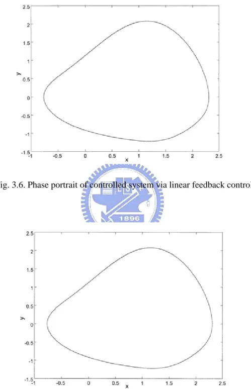
(18) For this purpose, open-loop strategies and close-loop feedback methods are used to control our system from chaos to order. (1) Controlling Chaos by Delayed Feedback Control Let us consider a dynamic system which can be simulated by ordinary differential equations. We imagine that the equations are unknown, but some scalar variable can be measured as a system output. The idea of this method, is that the difference D(t) between the delayed output signal y(t − τ ) and the output signal y(t) is used as a control signal. In other word, we adapt a perturbation of the form [17]: u(t ) = K [ y (t − τ ) − y (t )] = KD(t ). (3.1.2). here τ is a delay time. The difference between the delayed output signal and the output signal itself is used as a control signal. To achieve the periodic motion of the system, two parameters, namely, the time of delay τ and the weight K of the feedback, should be adjusted. For the autonomous system, it is easy to choose an appropriate τ to achieve the periodic state. From the simulation process, this method is more effective and applicable for control of chaos to the rotational machine. The numerical results are shown in Fig. 3.4 with K = 0.4.. (2) Controlling Chaos by Adaptive Control Algorithm (ACA) A simple and effective adaptive control algorithm is suggested [18], which utilizes an error signal proportional to the difference between the goal output and actual output of the system. The error signal governs the change of parameters of the system, which readjusts so as to reduce the error to zero. This method can be explained briefly. The system motion is set back to a desired state X s by adding dynamics on the control parameter P through the 16.

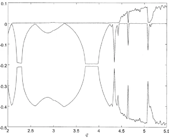
(19) evolution equation, .. P = εG ( X − X s ). (3.1.3). where the function G depends on the difference between X s and the actual output X , and ε indicates the stiffness of the control. The function G could be either linear or non-linear. In order to convert the dynamics of system (3.1.1) from chaotic motion to the desired periodic motion X s , the chosen paramer q is perturbed as q& = ε ( X − X S ). (3.1.4). if ε =0.005 , the system can reach the period-1 and period-2 easily shown as Fig. 3.5. It is clear that the desired periodic motion can be reached by adaptive control algorithm.. (3) Controlling Chaos by Linear Feedback Control A linear feedback control with a special form is used in this method. It is assumed that the input signal u(t) disturbs only the third equation in (3.1.1). and u (t ) = K 2 [ y i (t ) − y (t )] = K 2 D(t ). Here, y(t) is the chaotic output signal, y i (t ) is the periodic motion of system. The difference D(t ) between the signal y i (t ) and y (t ) is used as a control signal. Here K 2 is an adjustable weight of the feedback. By selecting the weight K 2 , we can convert chaotic behavior to periodic motion. We can control the chaotic behavior to period-1 motion by choosing K 2 =0.5 as shown in Fig. 3.6. (4) Controlling Chaos by Optimal Control. 17.

(20) Optimal control is a well-established engineering control strategy, and is useful for both linear and nonlinear system with linear or nonlinear controllers [6]. Now, we use a typical optimal control for a chaos control. We consider the equation(3.1.1) with a controller u and define the Hamilton function : H ( x , y , z , u, p ) = p T F ( x , y , z , u, t ). ,. p T = [ p1 p2 p3 ]. Following the variation principle of optimal control, we can obtain p1 y + p2 [dz 2 cos x +. 1 ( e + pz 2 ) sin 2 x − sin x − by ] = 0 2. − p2 ( 2dz cos x + pz sin 2 x ) = 0. (3.1.5) (3.1.6). This yield a non-trivial solution for ( p1 , p 2 ) if and only if 2dz cos x + pz sin 2 x = 0. (3.1.7). It gives an optimal surface singularly in the state space. This type of control assumes values on the two allowable boundaries (3.1.5) and (3.1.6) alternatively according to a switching surface. Locating system trajectories on the surface, a typical feedback control in the form u = −k b sgn[2dz cos x + pz sin 2 x ]. can be used. By adjusting the value of k b in the above controller with the signum function ⎧ 1 ⎪ sgn[v] = ⎨ 0 ⎪ −1 ⎩. if. v>0. if if. v=0 v<0. the chaotic motion can be controlled to periodic motion which we desired by modulating the value of k b . The simulation result is shown in Fig. 3.7 with k b = 1.5 .. 18.

(21) 3.1.4 Chaos Synchronization and Phase Synchronization A characteristic property of chaotic dynamics is the sensitive dependence on initial condition. Different initial conditions will cause different trajectories for the system. However, a few years ago Pecora and Carroll [5] shown that synchronization can be achieved for the chaotic systems. This interest phenomenon plays a significant role in the chaotic dynamics of communication signals and may be applied to the real-time recovery of signals that have been masked in a strange attractor and thus to encode communication. Other applications of synchronization of chaos also have expectative potential [7,8]. A natural way to develop synchronization for chaotic systems is through system decomposition. The coupled systems are decomposed into two subsystem as follows : ⎧ x&1 = y1 1 ⎪ 2 2 ⎨ y& 1 = dz1 cos x1 + ( e + pz1 ) sin 2 x1 − sin x1 − by1 2 ⎪ z& = ⎩ 1 q cos x1 − F. (drive). ⎧ x& 2 = y 2 1 ⎪ 2 2 ⎨ y& 2 = dz 2 cos x 2 + ( e + pz 2 ) sin 2 x 2 − sin x 2 − by 2 2 ⎪ z& = ⎩ 2 q cos x 2 − F. (response) (3.1.9). (3.1.8). In the following, several feedback based approaches are discussed. (1) Linear Feedback Synchronization In this approach, the error between the output of the identical drive and response is used as the control signal. The first equation of response(3.1.9) is combined with a linear feedback, while the equations of drive remain the same[6]. ⎧ x& 2 = y 2 + k ( x1 − x 2 ) 1 ⎪ 2 2 ⎨ y& 2 = dz 2 cos x 2 + ( e + pz 2 ) sin 2 x 2 − sin x2 − by 2 2 ⎪ z& = ⎩ 2 q cos x2 − F 19. (3.1.10).

(22) where k is the constant feedback gain. With k= 0.5, the trajectories of subsystems and the synchronization errors, e x = x 2 − x1 , e y = y 2 − y1 , and e z = z 2 − z1 , are shown in Fig. 3.8. In this case, k= 0.38 is a critical value,. below which no synchronization occurs. (2) Adaptive Feedback Synchronization In section 3.1.3, adaptive control strategies can direct a chaotic trajectory to stable orbits but not unstable ones. Therefore, it is possible to combine the feedback method for chaos synchronization [6]. For response (3.1.9), the linear feedback (3.1.10) is replaced by x& 2 = y 2 + k1 ( x1 − x 2 ) q& = k 2 ( y1 − y 2 ). (3.1.11). where q is the system parameter, and k 2 is a constant adaptive control gain to be determined in the design. Using this method, the response can synchronize the chaotic drive, as shown in Fig. 3.9. (3) Phase Synchronization Recently, the concept of phase, as well as phase synchronization, has been discussed in detail for chaotic oscillators [19,20]. If we project the attractor on plane (x,y), it has one rotation center shown in Fig. 3.1(c) and Fig. 3.10. The phase of the system can be defined as : φ = arctan. y x. (3.1.12). The phase can be easily calculated for each subsystem. Phase synchronization occurs when the phases of two oscillators have the relationship φ1 (t ) ≈ φ 2 (t ) with time. To determine the level of mismatch of phase synchronization, we use cross-correlation function ξ (τ ) with time shift τ [20]. ξ (τ ) =. y1 (t ) y 2 (t + τ ). ( y (t ) 2 1. y 22 (t ). (3.1.13). ). 1/ 2. 20.

(23) We study two coupled centrifugal governor systems with strength of coupling ε , x&1, 2 = y1, 2 y&1, 2 = dz12, 2 cos x1, 2 +. 1 ( e + pz12, 2 ) sin 2 x1, 2 − sin x1, 2 − by1, 2 + ε ( y 2,1 − y1, 2 ) 2. z&1, 2 = q cos x1, 2 − F. (3.1.14)` To examine phase synchronization, we modulate the coupling parameter ε in Eq. (3.1.14). Some numerical results are given in Fig. 3.11 with 0 < ε < 0.5 . Fig. 3.11(a) shows the maximum absolute difference of two phases. Obviously, the phases of two coupled systems are synchronizing in the region ε > 0.193 . Fig. 3.11(b) shows the maximum absolute difference of two trajectories. When ε > 0.193 , they are synchronization. Therefore, phase synchronization and full synchronization coincide for two coupled centrifugal governor systems. It means that the phases and amplitudes of two systems are equally correlated [20]. The cross-correlation function ξ (0) with τ = 0 is also shown in Fig. 3.11(c) correspondingly. It has been shown that phase synchronization for coupled Rössler systems is related to one of the zero Lyapunov exponents becoming negative [19]. But our simulation shows that there is not such a relationship for our system in Fig. 3.12. All signs of six Lyapunov exponents remain unchanged. This phenomenon indicates that a Lyapunov exponent decreasing from zero to negative cannot be used as a criterion for phase synchronization [20]. However, we can observe that when phase synchronization begins at ε = 0.193 , one of negative Lyapunov exponents approaches to zero, and becomes immediately negative again when ε > 0.193 in Fig. 3.12.. 21.

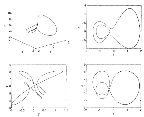
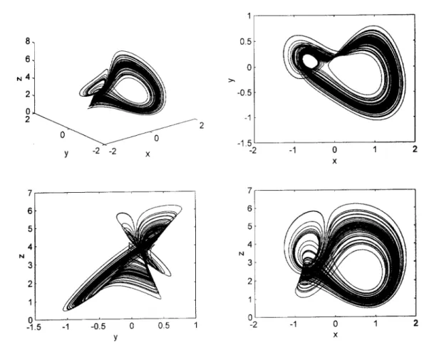
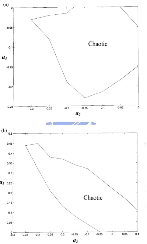
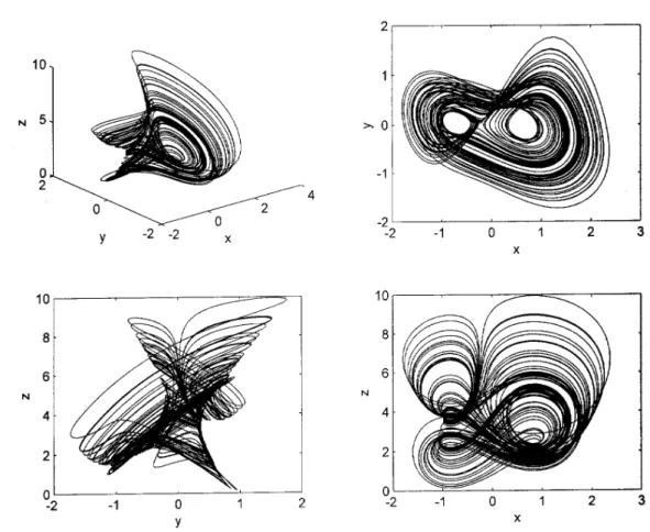
(24) 3.2 Anticontrol. and. Synchronization. of. Chaos. of. Autonomous System Anticontrol of chaos is making a nonchaotic dynamical system chaotic. This implies that the regular behaviors will be destroyed and replaced by chaotic behavior. In the real world, chaotic behavior is important. Examples include liquid mixing, humam heartbeat regulations, resonance prevention in mechanical systems and secure communication[11]. In this section, equation(3.1.1) are modified by the addition of a linear feedback and a nonlinear feedback to chaotify the system, respectively.. 3.2.1 Adding a Linear Feedback The state equations of the centrifugal governor system with a linear feedback controller are represented as x& = y + a1 x. 1 y& = dz 2 cos x + (e + pz 2 ) sin 2 x − sin x − by + a 2 y 2. (3.2.1). z& = q cos x − F + a3 z. Here a1 , a 2 , a3 are feedback gains and the values of parameters d , e, p, q, F , b are given as 0.008, 0.8, 0.04, 3, 2, 0.4, respectively. By numerical integration method, the phase portrait of the system, equation (3.2.1), is plotted in Fig. 3.13 for a1 = a 2 = a3 = 0. Clearly, the motion is periodic. But equation (3.2.1) exhibits both strange attractors and limit cycles for certain choices of a1 , a 2 and a3 . For example, when a1 = 0.2, a 2 = −0.1, a3 = −0.1 , one can observe a chaotic attractor as depicted in. Fig. 3.14. By simulation results, for certain interval of parameters, the system. 22.

(25) exhibits the strange attractor. Inspired by the consideration of chaotification, we found regions of specific feedback gains for which this system is chaotic as shown in Fig. 15.. 3.2.2 Adding a Nonlinear Feedback For our purpose, the nonlinear feedback controller, εx x , is added to the right-hand side of the first equation of equation(3.1.1). Then the system equations are represented as x& = y + εx x. 1 y& = dz 2 cos x + (e + pz 2 ) sin 2 x − sin x − by 2. (3.2.2). z& = q cos x − F. The system(3.2.2) is obtained which for certain value of ε (for example, 0.008 ≤ ε ≤ 0.032 ) has strange attractor by numerical solution. As illustrated in. Fig. 3.16, chaotic motion is observed from system(3.2.2) with ε = 0.01 .. 3.2.3 Chaos Synchronization The chaotic system(3.2.1) is decomposed into two subsystems as follows : drive system : x&1 = y1 + 0.2 x1 1 2 2 y&1 = dz1 cos x1 + (e + pz1 ) sin 2 x1 − sin x1 − by1 − 0.1y1 2 z&1 = q cos x1 − F − 0.1z1. (3.2.3). response system: x& 2 = y 2 + 0.2 x 2 1 2 2 y& 2 = dz 2 cos x 2 + (e + pz 2 ) sin 2 x 2 − sin x 2 − by 2 − 0.1 y 2 2 z& 2 = q cos x 2 − F − 0.1z 2. 23. (3.2.4).

(26) In the following, linear feedback, nonlinear feedback, adaptive feedback and backstepping design approaches are discussed. (1) Linear Feedback Synchronization In this approach, the error between the output of the identical drive and response is used as the control signal. For the unidirectional case, where only first equation of response system(3.2.4) is combined with a linear feedback, while the equations of drive remain the same[5]. x& 2 = y 2 + 0.2 x 2 + k1 ( x1 − x 2 ) 1 2 2 y& 2 = dz 2 cos x 2 + (e + pz 2 ) sin 2 x 2 − sin x 2 − by 2 − 0.1 y 2 2 z& 2 = q cos x 2 − F − 0.1z 2. (3.2.5). where k1 is the constant feedback gain. With k1= 0.2, the synchronization errors, e x = x 2 − x1 , e y = y 2 − y1 , and e z = z 2 − z1 , are shown in Fig. 3.17. In this case,. k1= 0.15 is a critical value, below which no completely synchronization occurs. (2) Nonlinear Feedback Synchronization The chaotic response system(3.2.4) by adding nonlinear coupling term are written as x& 2 = y 2 + 0.2 x 2 + k 2 sin( x1 − x 2 ) 1 2 2 y& 2 = dz 2 cos x 2 + (e + pz 2 ) sin 2 x 2 − sin x 2 − by 2 − 0.1 y 2 2 &z 2 = q cos x 2 − F − 0.1z 2. (3.2.6). With k2= 0.2, the synchronization errors are shown in Fig. 3.18. In this case, k2= 0.15 is a critical value, below which no completely synchronization occurs. (3) Adaptive Feedback Synchronization Some adaptive control strategies can direct a chaotic trajectory to stable orbits but not unstable ones. However, it is possible to combine the feedback method for chaos synchronization [21,22]. 24.

(27) For response system(3.2.4), the linear feedback (3.2.5) is replaced by x& 2 = y 2 + 0.2 x 2 + k 3 ( x1 − x 2 ) 1 2 2 y& 2 = dz 2 cos x 2 + (e + pz 2 ) sin 2 x 2 − sin x 2 − by 2 − 0.1 y 2 2 z& 2 = q cos x 2 − F − 0.1z 2 q& = k 4 ( y1 − y 2 ). (3.2.7). where the system parameter q is used as an adjustable function for adaptation, and k 4 is a constant adaptive control gain to be determined in the design. Using this method, the response can be synchronized by the chaotic drive, as shown in Fig. 3.19. (4) Backstepping design Backstepping design is a recursive procedure that combines the choice of a Lyapunov function for selecting a proper controller in chaos synchronization[23]. The drive system is expressed as Eq.(3.2.3) and a controller u is added to the right-hand side of the second equation of response system(3.2.4). Let the state errors between the response system and drive system be e x = x 2 − x1. e y = y 2 − y1. e z = z 2 − z1. (3.2.8). then error system can be derived as e& x = e y + 0.2e x e& y = d [cos x 2 (e z2 + 2 z1e z ) + + e& z =. z12 2 (e x + 2 x1e x )] + (e − 1)e x 2. p [sin 2 x 2 (e z2 + 2 z1e z ) + 2 z12 e x ] − (b + 0.1)e y + u + h.o.t. 2. (3.2.9). q e x − 0.1e z 2. If system(3.2.9) did not have u, it would have an equilibrium point(0,0,0). The problem of synchronization between drive and response system can be transformed into how to find a control law u for stabilizing the error variables. 25.

(28) of system(3.2.9) at the origin. First we consider the stability of system as following : e& z =. where e x. q e x − 0.1e z 2. (3.2.10). is regarded as a controller and it makes system(3.2.10). asymptotically stable. Choose Lyapunov function V1 (e z ) = e z2 / 2 . The derivative of V1 is q V&1 = −0.1e z2 + e z e x 2. (3.2.11). Assume controller e x = α 1 (e z ) and α 1 (e z ) = 0 , then V&1 = −0.1e z2 < 0. (3.2.12). makes system(3.2.10) asymptotically stable. Function α 1 (e z ) is an estimative function when e x is considered as a controller. The error between e x and α 1 (e z ) is w2 = e x − α 1 ( e z ). (3.2.13). Study (e z , w2 ) system q w2 − 0.1e z 2 w& 2 = e y + 0.2 w2. e& z =. (3.2.14). Consider e y = α 2 (e z , w2 ) as a controller in system(3.2.14). Choose Lyapunov function V2 (e z , w2 ) = V1 (e z ) + w22 / 2 . The derivative of V2 is q V&2 = −0.1e z2 + 0.2w22 + w2 e z + w2 e y 2. (3.2.15). q 2. If α 2 (e z , w2 ) = − e z − w2 , then V&2 = −0.1e z2 − 0.8w22 < 0. (3.2.16). makes system(3.2.14) asymptotically stable. Define the error variable w3 as. 26.

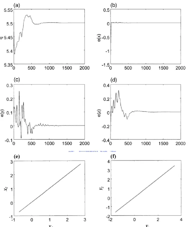
(29) w3 = e y − α 2 (e z , w2 ). (3.2.17). Study full dimension (e z , w2 , w3 ) system q w2 − 0.1e z 2 w& 2 = w3 + α 2 + 0.2 w2. e& z =. z12 2 ( w2 + 2 x1 w2 )] + (e − 1) w2 − (b + 0.1)( w3 + α 2 ) 2 dα 2 p + [sin 2 x 2 (e z2 + 2 z1e z ) + 2 z12 w2 ] − + u + h.o.t. 2 dt. w& 3 = d [cos x 2 (e z2 + 2 z1e z ) +. (3.2.18) where dα 2 q q = − ( w2 − 0.1e z ) − ( w3 + α 2 + 0.2 w2 ) dt 2 2. Choose Lyapunov function V3 (e z , w2 , w3 ) = V2 (e z , w2 ) + w32 / 2 . The derivative of V3 is p V&3 = −0.1e z2 − 0.8w22 + w3 [2 z1e z (q cos x 2 + sin 2 x 2 ) + ew2 2 (3.2.19) 2 dz1 dα 2 2 2 − (b + 0.1)( w3 + α 2 ) + ( w2 + 2 x1 w2 ) + pz1 w2 − + u ] + h.o.t. 2 dt. Let p sin 2 x 2 ) − ew2 2 dz 2 dα 2 − 1 ( w22 + 2 x1 w2 ) − pz12 w2 + dt 2. u = (b + 0.1)α 2 − 2 z1e z (q cos x 2 +. then V&3 = −0.1e z2 − 0.8w22 − (b + 0.1) w32 + h.o.t.. is quadric negative definite. Whereas x1 , z1 and x 2 are bounded, we can conclude that the equilibrium point(0,0,0) of error system(3.2.9) is locally asymptotically stable. For proper initial errors between drive and response systems, the initial errors will converge to zero and synchronization between 27.

(30) two chaotic subsystems will be achieved. The numerical results with initial condition ( x1 (0) = 1.42, y1 (0) = −2.1,. z1 (0) = 5.55 , x 2 (0) = 1.4, y 2 (0) = −2,. z 2 (0) = 5.5 ) are shown in Fig. 3.20.. (5) Parameter evaluation from time sequences In this section, we study another method to estimate the parameter of chaotic. system. by. a. random. optimization. method. for. chaos. synchronization[24]. For system(3.2.5), q is the unknown parameter and k1 is a coupling constant. The difference of the two time sequences is calculated as T. U = ∫ x 2 − x1 dt 2. 0. the integral time T is larger than a typical period of the chaotic oscillation in the governor system and the parameter q is randomly modified as q' = q + ζ. where ζ is a random number. We can obtain a time sequence x' 2 (t ) by numerical simulation of Eq.(3.2.5) with the modified parameter q' . Then the difference of the two time sequences is calculated as T. U ' = ∫ x' 2 − x1 dt 2. 0. If the difference U ' is smaller than U, the parameter is changed from q to q' . On the other hand, if the difference U ' is larger than U, the parameter is unchanged and kept to be q. The obtained parameter value is expected to be the desired parameter until the difference U becomes zero, i.e., complete chaos synchronization is achieved. Fig. 3.21 displays the minimum value of U with respect to the coupling constant k1 . The numerical simulation shows that the complete chaos synchronization x 2 (t ) = x1 (t ) occurs for k1 > 0.15 . This result is the same as that in section 3.2.3 (1). The difference U as a function of the parameter q for 28.

(31) k1 = 0.2 is shown in Fig. 3.22. The complete chaos synchronization is attained. when the value of U takes a minimum value 0 at q = 3. Time evolution of the parameter q by the random optimization process is shown in Fig. 3.23.. 3.3 Chaos, Control, Anticontrol and Synchronization of Chaos for the System with Time-Delay Chaos, control, anticontrol and synchronization of chaos for an autonomous rotational machine system with a hexagonal centrifugal governor and spring for which time-delay effect is considered are studied in this section. For a mass-spring system shown in Fig. 3.24, suppose m is not a particle. It has a length P2 − P1 . When the spring force acts on m at P1 in some instant t, m does not move immediately. This is because that when a force acts on the surface P1 of m, the stress waves propagate inside m. Usually the stress waves start from P1 and reflected at P2. After crisscross of stress waves inside m, acceleration of m becomes uniform, and m begins to move actually at this time. Let the time interval between the instant of exertion of the force on m and the instant at which m moves actually be τ . We have the equation of motion of time delay system as m&x&(t ) + kx(t − τ ) = 0 . This kind of time delay is considered in this section.. 3.3.1 Regular and Chaotic Dynamics of Time-Delay System The governor system(2.1.4) with time-delay considered can be modeled by the following delay differential equations: φ& = ϕ r l. ϕ& = ω 2 cos φ + ω 2 sin φ cos φ −. 2k g (1 − cos φ t −τ ) sin φ − sin φ − cϕ m l. ω& = q cos φ − F 29. (3.3.1).

(32) In nonlinear dynamical systems, variation of system parameters may cause sudden change in the qualitative behavior of their state. The state change is referred to as a bifurcation and the parameter value at which the bifurcation occurs is called the bifurcation value. Denoting φ = x, φ& = y, ω = z, equation (3.3.1) is rewritten in the form x& = y y& =. r 2 2k g z cos x + z 2 sin x cos x − (1 − cos xt −τ ) sin x − sin x − cy l m l. (3.3.2). z& = q cos x − F. Here q is considered as the control parameter to be varied when the values of parameters r , l , k , m, F , c are given as 0.4, 2, 20, 2, 1.942, 0.4, respectively. The phase portrait is the evolution of a set of trajectories emanating from various initial conditions in the state space. When the solution reaches steady state, the transient behavior disappears. By numerical integration method, the phase portrait of the system, equation (3.3.2), is plotted in Fig. 3.25(a) for q = 3. Clearly, the motion is periodic. But Fig. 3.25(b) for q = 5.5 shows the chaotic states. Furthermore the power spectrum is a continuous broad-band one shown in Fig. 3.26(b) as q = 5.5. The noise-like spectrum is the characteristic of chaotic dynamical system.. 3.3.2 Controlling Chaos It has been shown that the time-delay autonomous system exhibited both regular and chaotic motion in previous section. Usually chaos is unwanted or undesirable. In order to improve the performance of a dynamic system or to avoid the chaotic phenomena, we need to control a chaotic motion to become a periodic motion which is beneficial for working with a particular condition. For 30.

(33) this purpose, two methods are used to control the time-delay system from chaos to order. (1) Controlling Chaos by Adaptive Control Algorithm (ACA) A simple and effective adaptive control algorithm is suggested [18], which utilizes an error signal proportional to the difference between the goal output and actual output of the system. The error signal governs the change of parameters of the system, which readjusts so as to reduce the error to zero. This method can be explained briefly. The system motion is set back to a desired state X s by adding dynamics on the control parameter P through the evolution equation, .. P = εG ( X − X s ). (3.3.3). where the function G depends on the difference between X s and the actual output X , and ε indicates the stiffness of the control. The function G could be either linear or non-linear. In order to convert the dynamics of system (3.3.2) from chaotic motion to the desired periodic motion X s , the chosen paramer q is perturbed as q& = K 1 ( X − X S ). (3.3.4). If K1=0.5 , the system can reach the period-1 easily shown as Fig. 3.27. It is clear that the desired periodic motion can be reached by adaptive control algorithm. (2) Controlling Chaos by Linear Feedback Control A linear feedback control with a special form is used in this method. It is assumed that the input signal u(t) disturbs only the third equation in (3.3.2). and u (t ) = K 2 [ y i (t ) − y (t )] = K 2 D(t ). (3.3.5) 31.

(34) Here, y(t) is the chaotic output signal, y i (t ) is the periodic motion of system. The difference D(t ) between the signal y i (t ) and y (t ) is used as a control signal. Here K 2 is an adjustable weight of the feedback. By selecting the weight K 2 , we can convert chaotic behavior to periodic motion. We can control the chaotic behavior to period-1 and period-2 motion by choosing K 2 =5 and 0.5, respectively, as shown in Fig. 3.28.. 3.3.3 Chaos Synchronization The chaotic system is decomposed into two subsystems as follows : drive system: x&1 = y1. y&1 =. 2k g r 2 2 (1 − cos x1t −τ ) sin x1 − sin x1 − cy1 (3.3.6) z1 cos x1 + z1 sin x1 cos x1 − l m l. z&1 = q cos x1 − F. response system: x& 2 = y 2. y& 2 =. 2k g r 2 2 (1 − cos x 2 t −τ ) sin x 2 − sin x 2 − cy 2 z 2 cos x 2 + z 2 sin x 2 cos x 2 − l m l. z& 2 = q cos x 2 − F. (3.3.7). In the following, linear and nonlinear feedback based approaches are discussed. (1) Linear Feedback Synchronization In this approach, the error between the output of the identical drive and response is used as the control signal. For the unidirectional case, where only first equation of response(3.3.7) is combined with a linear feedback, while the equations of drive remain the same. x& 2 = y 2 + K ( x1 − x 2 ). 32.

(35) y& 2 =. r 2 2k g 2 z 2 cos x 2 + z 2 sin x 2 cos x 2 − (1 − cos x 2 t −τ ) sin x 2 − sin x 2 − cy 2 l m l. z& 2 = q cos x 2 − F. (3.3.8). where K is the constant feedback gain. With K= 3, the trajectories of subsystems and the synchronization errors, e x = x2 − x1 , e y = y 2 − y1 , and e z = z 2 − z1 , are shown in Fig. 3.29. In this case, K= 2.75 is a critical value,. below which no synchronization occurs. Then we consider the two identical systems which are coupled together. The mutually coupled chaotic systems by adding linear coupling term are written as drive system: x&1 = y1 + K ( x 2 − x1 ). y&1 =. r 2 2k g 2 z1 cos x1 + z1 sin x1 cos x1 − (1 − cos x1t −τ ) sin x1 − sin x1 − cy1 (3.3.9) l m l. z&1 = q cos x1 − F. response system: x& 2 = y 2 + K ( x1 − x 2 ). y& 2 =. 2k g r 2 2 (1 − cos x 2 t −τ ) sin x 2 − sin x 2 − cy 2 z 2 cos x 2 + z 2 sin x 2 cos x 2 − l m l. z& 2 = q cos x 2 − F. (3.3.10). The simulation result show that generalized synchronization occurs when K = 0.8 ～2.75, and two chaotic systems are complete synchronization when K > 3.75. With K= 1.5 and 3, the synchronization errors are shown in Fig. 3.30 and Fig. 3.31, respectively. (2) Nonlinear Feedback Synchronization The mutually coupled chaotic systems by adding nonlinear coupling term are written as. 33.

(36) drive system: x&1 = y1 + K sin( x 2 − x1 ). y&1 =. r 2 2k g 2 z1 cos x1 + z1 sin x1 cos x1 − (1 − cos x1t −τ ) sin x1 − sin x1 − cy1 l m l. (3.3.11) z&1 = q cos x1 − F. response system: x& 2 = y 2 + K sin( x1 − x 2 ). y& 2 =. r 2 2k g 2 z 2 cos x 2 + z 2 sin x 2 cos x 2 − (1 − cos x 2 t −τ ) sin x 2 − sin x 2 − cy 2 l m l. z& 2 = q cos x 2 − F. (3.3.12). With K= 1.5, the trajectories of subsystems and the synchronization errors are shown in Fig. 3.32. (3) Phase Synchronization Recently, the concept of phase, as well as phase synchronization, has been discussed in detail for chaotic oscillators [19,20]. If we project the attractor on plane (x,y), it has one rotation center shown in Fig. 3.25(b). The phase of the system can be defined as : φ = arctan. y − yc x − xc. (3.3.13). where the point ( xc , y c ) is the rotation center. The phase can be easily calculated for each subsystem, and the mean frequency also defined as [10] φ (T ) − φ (0) Ω =< φ& >= lim T →∞ T. (3.3.14). Phase synchronization occurs when the phases of two oscillators have the relationship. φ1 (t ) ≈ φ 2 (t ). with time, i.e., frequency-locking state for. ∆Ω = Ω1 − Ω 2 → 0 .. We study two coupled centrifugal governor systems with strength of 34.

(37) coupling K, x&1, 2 = y1, 2 + K ( x 2,1 − x1, 2 ) y&1, 2 =. r 2k 2 2 z1, 2 cos x1, 2 + z1, 2 sin x1, 2 cos x1, 2 − (1 − cos x1, 2 t −τ ) sin x1, 2 l m g − sin x1, 2 − cy1, 2 l. (3.3.15). z&1, 2 = q cos x1, 2 − F. To examine phase synchronization, we modulate the coupling parameter K in Eq. (3.3.15). Some numerical results are given in Fig. 3.33. For the unidirectional case, Fig. 3.33(a) shows the maximum absolute difference of mean frequency between two trajectories. Obviously, the phases of two systems are synchronizing in the region K > 3.9 . Fig. 3.33(b) shows the maximum absolute difference of mean frequency between the mutually coupled chaotic systems. When K > 1.4 , they are phase synchronization. Therefore, phase synchronization is easily achieved in mutually coupled chaotic systems.. 3.3.4 Anticontrol of Chaos Sometimes, chaos is not only useful but actually important. Besides secure communication and information processing, chaos is desirable in many applications of liquid mixing while the required energy is minimized. For this purpose, making a non-chaotic dynamical system chaotic is called “anticontrol of chaos”. For our system(3.3.2), it is periodic motion with q = 3. The feedback controller used is a simple triangle function shown in Fig. 3.34(a), the period motion becomes chaotic shown in Fig. 3.34(b).. 35.

(38) 3.4 Chaos, Controlling Chaos and Synchronization of Chaos of Nonautonomous System 3.4.1 Regular and Chaotic Dynamics of Nonautonomous System In previous sections, the load torque is assumed to be constant for the system. Another condition can be considered. The load torque is now not constant but is represented by a constant term and a harmonic term F + a sin ω t , where F , a, ω are constants.Equation (3.1.1) is rewritten in the form x& = y 1 ( e + pz 2 ) sin 2 x − sin x − by 2 z& = q cos x − F − a sin ω t y& = dz 2 cos x +. (3.4.1). where d = 0.008, e = 0.8, p = 0.04, F = 1.942, a = 0.6, b = 0.4, ω = 1.0 . (1)Phase Portraits , Poincaré Map and Power Spectrum The phase portrait is the evolution of a set of trajectories emanating from various initial conditions in the state space. When the solution reaches steady state, the transient behavior disappears. The idea of transforming the study of continuous systems into the study of an associated discrete system was presented by Henri Poincaré. One of many advantages of Poincaré map is to reduce dimensions of the dynamical system. The solution of period-1T in the phase plane will become one point in the Poincaré map. By using fourth order Runge-Kutta numerical integration method, the phase plane and Poincaré map of the system, equation (3.4.1), is plotted in Fig. 3.35(a), (b) for q = 2.07, 2.14, respectively. Clearly, the motion is periodic. But Fig. 3.35(c), (d) for q = 2.21 show the chaotic states. Because the Poincaré map is neither a finite set of points nor a closed orbit, the motion may be chaotic. A valuable technique for the identification and characterization of the system is the power spectrum. This representation is useful for dynamical 36.

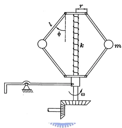
(39) analysis. The periodic motion of nonautonomous system are observed by the portraits of power spectrum in Fig. 3.36(a) for q = 2.07. The solution of system is period-1T, and the power spectrum exhibits a strong peak at the forcing frequency together with super-harmonic frequencies. As the q increase, the period-1T changes to period-2T and the peak arises at one half forcing frequency, twice of principal period in the power spectrum. Apparently, the spectrum of the periodic motion only consists of discrete frequencies. As q = 2.21 chaos occurs, the points of Poincaré map become obviously irregular. The spectrum is a broad band and the peak is still presented at the fundamental frequency shown in Fig. 3.36(b). The noise-like spectrum is the characteristic of chaotic dynamical system. (2) Bifurcation Diagram and Parametric Diagram In the previous section, the information about the dynamics of the non-linear system for specific values of the parameters is provided. The dynamics may be viewed more completely over a range of parameter value. As the parameter is changed, the equilibrium points can be created or destroyed, or their stability can be lost. The phenomenon of sudden change in the motion as a parameter is varied is called bifurcation, and the parameter values at which they occur are called bifurcation points. The bifurcation diagram of the non-linear system of equation (3.4.1) is depicted in Fig. 3.37. It is calculated by the fourth order Runge-Kutta numerical integration and plotted against the q ∈ [2.07,2.21] with the incremental value of q is 0.0002. At each q, the points of Poincaré map in the transient state of motion are discarded. The period-doubling bifurcation first appears for q ≈ 2.095 . In this model, a sequence of period-doubling bifurcations occurs and leads to chaos as the system parameter is varied. 37.

(40) Further, the parameter values, damping coefficient and forcing frequency will also be varied to observe the behaviors of bifurcation of the system. By varying simultaneously any two of the three parameters, amplitude of the external torque, damping coefficient, and forcing frequency, the parametric diagrams are described and shown as Fig. 3.38(a), (b). The enriched information of the behaviors of the system can be obtained from the diagrams. (3) Lyapunov Exponent and Lyapunov Dimension The Lyapunov exponent may be used to measure the sensitive dependence upon initial conditions. It is an index for chaotic behavior. Different solutions of dynamical system, such as fixed points, periodic motions, quasiperiodic motion, and chaotic motion can be distinguished by it. If two chaotic trajectories start close to one another in phase space, they will move exponentially away from each other for small times on the average. Thus, if d0 is a measure of the initial distance between the two starting points, the distance is d (t ) = d 0 2 λt . The symbol λ is called Lyapunov exponent. The divergence of chaotic orbits can only be locally exponential, because if the system is bounded, d (t ) cannot grow to infinity. A measure of this divergence of orbits is that the. exponential growth at many points along a trajectory has to be averaged. When d (t ) is too large, a new 'nearby' trajectory d 0 (t ) is defined. The Lyapunov. exponent can be expressed as: λ=. 1 t N − t0. N. ∑ log k =1. 2. d (t k ) . d 0 (t k −1 ). The signs of the Lyapunov exponents provide a qualitative picture of a system dynamics. The criterion is. λ>0. (chaotic),. λ≤0. (regular motion).. 38.

(41) The periodic and chaotic motions can be distinguished by the bifurcation diagram, while the quasiperiodic motion and chaotic motion may be confused. However, they can be distinguished by the Lyapunov exponent method. The Lyapunov exponents of the solutions of the non-linear dynamical system, equation (3.4.1), are plotted in Figure 3.39 as q ranges from 2.07 to 2.21. For the system studied the sum of the four Lyapunov exponents is equivalent to the negative damping coefficient -0.4. If the value of Lyapunov exponent is greater than zero, it is chaos, otherwise periodic solution. Observably, the chaotic motion can be found in Fig. 3.39 for q close to 2.2. There are a number of different fractional-dimension-like quantities, including the information dimension, Lyapunov dimension, and the correlation exponent, etc; the difference between them is often small. The Lyapunov dimension is a measure of the complexity of the attractor. It has been developed by Kaplan and Yorke that the Lyapunov dimension d L is introduced as dL. ∑ = j+. j. λ i =1 i. λ j +1. ,. where j is defined by the condition that j. ∑λ. i. i =1. j +1. >0. and. ∑λ. i. < 0.. i =1. The Lyapunov dimension for a strange attractor is a non-integer number. The Lyapunov dimension and the Lyapunov exponent of the non-linear system are listed in Table 1 for different value of q.. 39.

(42) Table 1 Lyapunov exponents and Lyapunov dimensions of the system for different q. q. λ1. λ2. λ3. λ4. ∑λ. 2.07 2.14 2.185 2.21. -0.0431 -0.0407 -0.0506 0.0351. 0 0 0 0. -0.0437 -0.0553 -0.0764 -0.1206. -0.3132 -0.304 -0.273 -0.3145. -0.4 -0.4 -0.4 -0.4. dL. i. 1 Period-1 1 Period-2 1 Period-4 2.291 Chaos. 3.4.2 Controlling Chaos Several interesting non-linear dynamic behaviors of the system have been discussed in previous sections. It has been shown that the forced system exhibited both regular and chaotic motion. Usually chaos is unwanted or undesirable. In order to improve the performance of a dynamic system or to avoid the chaotic phenomena, we need to control a chaotic motion to become a periodic motion which is beneficial for working with a particular condition. It is thus of great practical importance to develop suitable control methods. Very recently much interest has been focused on this type of problem - controlling chaos. For this purpose, open-loop strategies and close-loop feedback methods are used to control our system from chaos to order. (1) Controlling Chaos by Addition of Constant Motor Torque Interestingly, one can even add just a constant term to control or quench the chaotic attractor to a desired periodic one in typical non-linear nonautonomous system. In practice, An external input u is a torque on the axis of rotational machine. The equation (3.4.1) can be rewritten as x& = y 1 y& = dz 2 cos x + (e + pz 2 ) sin 2 x − sin x − by 2 z& = q cos x − F − a sin ω t + u. 40. (3.4.2).

(43) It ensures effective control in a very simple way. In order to understand this simple controlling approach in a better way, this method is applied to the system (3.4.2) numerically. We add the constant motor torque u=T into the third equation of equation (3.4.2). In the absence of the constant motor torque, the system exhibits chaotic behavior under the parameter condition, q = 2.21. If one considers the effect of the constant motor torque T by increasing it from zero upwards, the chaotic behavior is then altered. In Fig. 3.40, the bifurcation diagram is shown. It is clear that the system returns to regular motion, when the constant motor torque T is great than 0.03. (2) Controlling Chaos by the Addition of Periodic Force One can control system dynamics by addition of external periodic force in the chaotic state. For our purpose, the added periodic force, u = vsin ω~t , is given, the system can then be investigated by numerical solution, with the remaining parameter fixed. We examine the change in the dynamics of the system as a function of v for fixed ω~ = 2 . The bifurcation diagram is shown in Fig. 3.41. It presents the return of the chaotic behavior to periodic motion while the value of v increase form zero upward. (3) Controlling Chaos by the Addition of Periodic Impulse Input Following the sense of previous sections, another open loop control method is given. A technique for suppressing chaos is to apply a periodic impulse input to the system[6]. Consider the system of the form (3.4.2) and assume that the system is controlled by a periodic impulse input ∞. u = ρ ∑ δ (τ − iTd ). (3.4.3). i =0. where ρ is a constant impulse intensity, Td is the period between two 41.

(44) consecutive impulses, and δ is the standard delta function. With different values of ρ and Td the controlled system can be stabilized at different periodic orbits. For example, we fix the parameter Td = 0.01 and adjust impulse intensity ρ , the chaotic behavior disappear. The bifurcation diagram is shown in Fig. 3.42. (4) Controlling Chaos by Delayed Feedback Control Let us consider a dynamic system which can be simulated by ordinary differential equations. We imagine that the equations are unknown, but some scalar variable can be measured as a system output. The idea of this method, is that the difference D(t) between the delayed output signal y(t − τ ) and the output signal y(t) is used as a control signal. In other word, we adapt a perturbation of the form[17]: u(t ) = K [ y (t − τ ) − y (t )] = KD(t ). (3.4.4). Here τ is a delay time. Choose an appropriate weight K and τ of the feedback one can achieve the periodic state. We can control the chaotic motion to any assigned periodic motion rapidly by this method. The dependence of the bifurcation diagram on K for period-1 time delay is shown in Fig. 3.43. This control is achieved by the use of the output signal, which is fed in a special form into the system. The difference between the delayed output signal and the output signal itself is used as a control signal. Only a simple delay line is required for this feedback control. To achieve the periodic motion of the system, two parameters, namely, the time of delay τ and the weight K of the feedback, should be adjusted. From the simulation process, this method is more effective and applicable for control of chaos to the rotational machine. (5) Controlling Chaos by Adaptive Control Algorithm (ACA) 42.

(45) Recently a simple and effective adaptive control algorithm is suggested, which utilizes an error signal proportional to the difference between the goal output and actual output of the system. The error signal governs the change of parameters of the system, which readjusts so as to reduce the error to zero. This method can be explained briefly. The system motion is set back to a desired state X s by adding dynamics on the control parameter P through the evolution equation, .. P = εG ( X − X s ). (3.4.5). where the function G depends on the difference between X s and the actual output X , and ε indicates the stiffness of the control. The function G could be either linear or non-linear. In order to convert the dynamics of system (3.4.1) from chaotic motion to the desired periodic motion X s , the chosen paramer q is perturbed as q& = ε ( X − X S ). (3.4.6). if ε =0.2 , the system can reach the period-1 and period-2 easily shown as Fig. 3.44 and Fig. 3.45. It is clear that the desired periodic motion can be reached by adaptive control algorithm. (6) Controlling Chaos by Bang-Bang Control Define error function as follow: e( t ) = X ( t ) − X ( t − T ). (3.4.7). where T is the external torque frequency. Define V (t ) = e(t ) 2 which is always positive or zero. V& = 2 ⋅ e(t ) ⋅ e&(t ). 43.

(46) If V& < 0 then V will approach zero, i.e. e(t ) → 0 . It means that x(t ) approaches x(t − Ti ) and the periodic behavior is achieved. The control law can be determined as follow: x& = F1 ( x, y , z, t ) y& = F2 ( x, y , z, t ). z& = F3 ( x, y , z , t ) + u. (3.4.8). if e(t ) ≤ δ , u(t ) = 0 else if e(t ) > δ then u (t ) = − K1 F3 ( x, y , z, t ) − z&(t − T ). when e(t ) > 0. u (t ) = K1 F3 ( x, y , z, t ) − z&(t − T ). when e(t ) < 0. When the trajectory close to our periodic orbit, the control signal is approach to zero. Fig. 3.46 show the phase portrait and Poincaré map for K 1 =0.03.. (7) Controlling Chaos by External Force Control A feedback control with a periodic external force of a special form is used in this method[17]. It is assumed that the input signal u(t) disturbs only the third equation in (3.4.2). and u (t ) = K 2 [ y i (t ) − y (t )] = K 2 D(t ). Here, y(t) is the chaotic output signal, y i (t ) is the periodic motion of system. The difference D(t ) between the signal y i (t ) and y (t ) is used as a control signal. Here K 2 is an adjustable weight of the feedback. By selecting the weight K 2 , we can convert chaotic behavior to periodic motion, the 44.

(47) bifurcation diagram is shown in Fig. 3.47. We can control the chaotic behavior to period-1 motion by choosing K 2 =0.9. We also can convert the chaotic motion to period-2 and period-4 for a suitable K 2 . (8) Controlling Chaos by Optimal Control Optimal control is a well-established engineering control strategy, and is useful for both linear and nonlinear system with linear or nonlinear controllers[6]. Now, we use a typical optimal control for a chaos control. We consider the equation(3.4.8) with a controller u and define the Hamilton function : H ( x , y , z , u, p ) = p T F ( x , y , z , u, t ). ,. p T = [ p1 p2 p3 ]. Following the variation principle of optimal control, we can obtain p1 y + p2 [dz 2 cos x +. 1 ( e + pz 2 ) sin 2 x − sin x − by ] = 0 2. (3.4.9). − p2 ( 2dz cos x + pz sin 2 x ) = 0. (3.4.10) This yield a non-trivial solution for ( p1 , p 2 ) if and only if 2dz cos x + pz sin 2 x = 0. (3.4.11). It gives an optimal surface singularly in the state space. This type of control assumes values on the two allowable boundaries (3.4.9) alternatively according to a switching surface. Locating system trajectories on the surface, a typical feedback control in the form u = −k b sgn[2dz cos x + pz sin 2 x ]. can be used. By adjusting the value of k b in the above controller with the signum function. 45.

(48) ⎧ 1 ⎪ sgn[v] = ⎨ 0 ⎪ −1 ⎩. if. v>0. if if. v=0 v<0. the chaotic motion can be controlled to periodic motion which we desired by the bifurcation diagram as shown in Fig. 3.48.. 3.4.3 Chaos Synchronization Recall from Section 3.1.4, a natural way to develop synchronization for chaotic systems is through system decomposition. The coupled systems are decomposed into two subsystem as follows : ⎧ x&1 = y1 1 ⎪ 2 2 ⎨ y&1 = dz1 cos x1 + (e + pz1 ) sin 2 x1 − sin x1 − by1 2 ⎪ z& = ⎩ 1 q cos x1 − F − a sin ω t. ⎧ x& 2 = y 2 1 ⎪ 2 2 ⎨ y& 2 = dz 2 cos x 2 + (e + pz 2 ) sin 2 x 2 − sin x 2 − by 2 2 ⎪ z& = ⎩ 2 q cos x 2 − F − a sin ω t. (drive) (3.4.12). (response) (3.4.13). By linear feedback approach, the error between the output of the identical drive and response is used as the control signal. The first equation of response(3.4.13) is combined with a linear feedback, while the equations of drive remain the same. ⎧ x& 2 = y 2 + k ( x1 − x 2 ) 1 ⎪ 2 2 ⎨ y& 2 = dz 2 cos x 2 + (e + pz 2 ) sin 2 x 2 − sin x 2 − by 2 2 ⎪ z& = ⎩ 2 q cos x 2 − F − a sin ω t. (3.4.14). where k is the constant feedback gain. Complete synchronization between the two chaotic systems can be observed with k= 0.2, the trajectories of the 46.

(49) synchronization errors, e x = x 2 − x1 , e y = y 2 − y1 , and e z = z 2 − z1 , are shown in Fig. 3.49.. 47.