國
立
交
通
大
學
資訊工程學系
碩
士
論
文
在即時多處理器系統上之有效的動態排程演算法
An Effective Dynamic Task Scheduling Algorithm for Real-Time
Multiprocessor Systems
研究生:柳文斌
d
指導教授:陳 正 教授
在即時多處理器系統上之有效的動態排程演算法
An Effective Dynamic Task Scheduling Algorithm for Real-Time
Multiprocessor Systems
研究生 :柳文斌
Student:
Wen-Pin
Liu
指導教授:陳 正 教授
Advisor: Prof. Cheng Chen
國立交通大學
資訊工程學系
碩士論文
A Thesis
Submitted to Department of Computer and Information Science College of Electrical Engineering and Computer Science
National Chiao Tung University in partial Fulfillment of the Requirements
for the Degree of Master
in
Computer Science and Information Engineering June 2005
Hsinchu, Taiwan, Republic of China
在即時多處理器系統上之有效的動態排程演算法
研究生 :柳文斌 指導教授:陳 正 教授
國立交通大學資訊工程學系碩士班
摘要
在即時系統中的工作,不但要求計算結果正確,而且必須在一定的時限內完成。 由於在一個多處理器的即時系統中的工作,如果無法在時限內被正確的被執行並傳回 計算結果會導致嚴重的後果,所以具有容錯能力的工作排程演算法是非常重要的。主 從模型(Primary Backup model)是一種常用的容錯排程方式。這類的排程法會為工 作安排額外的備份,因此系統資源的需求會較大。本論文即是提出了一個動態排程演 算法,並使之能夠動態調整備份工作的數量。其目的是為了讓更多的工作在時限內被 正確執行並降低系統資源的要求,為此,我們提出了負載回饋的調整機制,依據當前 系統的負載程度來決定是不是要安排額外的備份工作。此方法採取的是折衷原則,藉 由減少備份工作的安排以達到節省系統資源的目的,並將其用來執行更多的工作,有 效提高工作完成比。為了回收並有效利用配置給備份工作的系統資源,我們也提出了 一個等候機制,讓工作在佇列中等待系統資源被釋放,直到工作本身的完成時限無法 被滿足為止。我們以模擬的方式來評估演算法的效能,結果顯示,在大部分的情況下, 我們的方法比其他現有的演算法具有更好的工作完成比,但是容錯的能力會稍微下降。An Effective Dynamic Task Scheduling Algorithm for
Real-Time Multiprocessor Systems
Student: Wen-Pin Liu Advisor: Prof. Cheng Chen Institute of Computer Science and Information Engineering
National Chiao Tung University
Abstract
Real-time systems are defined as those systems in which the correctness of the system depends not only on the logical result of computation, but also on the time at which the results are produced. Task scheduling on real-time multiprocessor systems with fault-tolerant requirements is an important problem due to the catastrophic consequences of not tolerating faults. Primary Backup model is commonly used to schedule real-time tasks with fault-tolerant requirements. In such scheme, redundant copies of tasks are scheduled and more computing resources are required. In this thesis, we propose an effective dynamic scheduling algorithm, named Loading-driven Adaptive Scheduling Algorithm (LASA), which has an adaptive fault-tolerant mechanism to control when redundant (backup) copies of tasks will be scheduled or not. For the purpose of conserving computing resources and achieving higher Guarantee Ratio, the proposed loading-driven adaptation strategy takes the system loading into consideration and makes a trade-off between rejecting tasks and accepting them without backup copies. In order to improve the utilization of reclaimed computing resources from redundant copies, we also propose the task deferment mechanism by adding a waiting queue to the scheduling scheme. A task can be left in the waiting queue until some processors become available or its deadline becomes unable to be met. To evaluate the performance of our proposed algorithm, we have constructed a simulation environment to study it and found that our algorithm outperforms other previous work.
Acknowledgements
I wish to thank my advisor, Professor Cheng Chen, whose inspiration led to the development of this text. Also, I’d like to thank Professor Jyh-Jiun Shann and Professor Guan-Joe Lai for their comments.
Grateful thanks are due to those who read drafts of this thesis, and made helpful comments. These include Wei-Fan Yang, Chia-Chun Lee, Zhe-Ying Laio, and Ming-Xian Thai. I’m fortunate to have such delightful fellows. Especial thanks are due to Yi-Hsuan Lee, who has devoted so much time to reading and checking this thesis.
Table of Contents
摘要 ...i Abstract...ii Acknowledgements ...iii Table of Contents...iv List of Figures...vi Chapter 1 Introduction... 1Chapter 2 System Model and Related Work... 4
2.1 System model ... 4
2.1.1 Task model... 4
2.1.2 Scheduler model ... 5
2.1.3 Fault model ... 5
2.2 Related work... 6
2.2.1 The heuristic dynamic scheduling problem... 6
2.2.2 Myopic scheduling algorithm... 8
2.2.3 Backup overloading and backup deallocation ... 9
2.2.4 DMA and FTMA ... 9
2.2.5 DNA ... 10
2.2.6 Real-time self-adjusting dynamic scheduling algorithm ... 11
2.2.7 Value-based scheduling scheme ... 11
2.2.8 Feedback-based adaptive scheduling scheme... 12
Chapter 3 Loading-driven Adaptive Scheduling Algorithm (LASA)... 13
3.1 Overview ... 13
3.2 The heuristic function for task selection... 16
3.3 The processor allocation strategies... 17
3.4 Task deferment and rejection in the waiting queue ... 19
3.5 The loading driven adaptation strategy ... 20
Chapter 4 Preliminary Performance Evaluations ... 25
4.1 Simulation overview... 25
4.1.1 The task generator ... 25
4.1.2 The simulator ... 26
4.2 Result and analysis ... 29
4.2.1 Guarantee Ratio ... 30
4.2.2 The trade-off between reliability and schedulability ... 32
4.2.3 The effect of failure rate ... 35
5.1 Conclusion ... 37 5.2 Future work ... 38 References ...40
List of Figures
Fig. 2.1 The scheduler model... 5
Fig. 2.2 The concept of heuristic scheduling problem... 7
Fig. 2.3 The backup overloading... 9
Fig. 3.1 A loading-driven adaptive scheduler... 14
Fig. 3.2 The loading-driven adaptive scheduling algorithm... 15
Fig. 3.3 A workload... 17
Fig. 3.4 The partial schedule at time = 11... 17
Fig. 3.5 The current schedule at time = 16... 19
Fig. 3.6 The complete schedule at time = 70... 20
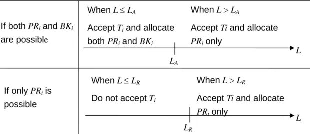
Fig. 3.7 The relationship among L, threshold, and scheduling strategies... 22
Fig. 3.8 The schedule at time = 54... 23
Fig. 3.9 The schedule at time = 70... 23
Fig. 4.1 The range of a randomly chosen deadline... 26
Fig. 4.2 Parameters of the task generator... 26
Fig. 4.3 Parameters for fault events... 27
Fig. 4.4 The architecture of the simulator... 28
Fig. 4.5 Effect of task load... 30
Fig. 4.6 Effect of laxity... 31
Fig. 4.7 Effect of number of processor... 31
Fig. 4.8 Number of primary-only task... 33
Fig. 4.9 Effect of threshold values... 34
Fig. 4.10 Effect of threshold values... 34
Fig. 4.11 Effect of failure probability on LASA The 3-tuple means (λ, m, R), which indicating different workload scenarios... 36
Chapter 1 Introduction
Real-time systems require both functionally correct executions and the results that are produced on time [1]. Because of their capability for high performance and reliability, multiprocessors and multi-computers systems have emerged as a powerful computing means for the real-time applications, such as autopilot systems, satellite and nuclear plant control [8, 13-14]. In such systems, the problem of the real-time task scheduling is to determine when and on which processor a task is executed so that the execution satisfies its deadline requirements. The scheduling can be performed either statically or dynamically [1]. In static algorithms, the assignment of the tasks to processors and the time at which the tasks start execution are determined a priori. Static algorithms are often used to schedule the periodic tasks but not applicable to the aperiodic tasks whose arrival times and deadlines are not known until they really arrive at the system. Therefore, a dynamic scheduling algorithm is required for scheduling the aperiodic tasks. Since there does not exist an optimal scheduling algorithm for dynamically arrival tasks [1, 16], and we need to find a feasible schedule quickly, heuristic approaches are taken.
If the scheduler can reserve enough computing resources for the task to be finished before its deadline, we say that the task is guaranteed or accepted [4-5]. Meanwhile, to guarantee newly arrival tasks must not jeopardize the previously guaranteed tasks. When too many tasks arrive at one time, the scheduler can not guarantee that all tasks meet their deadlines and it must reject some tasks. The task rejection invokes the error handling routines for fixing it and causes the overall system performance degradation. The most important objective of a dynamic scheduling algorithm is to guarantee as many tasks meeting their deadlines as possible [5, 11-12].
Due to the critical nature of real-time tasks, several techniques have evolved for fault-tolerant scheduling [4, 18-19]. In Primary Backup (PB) model, one primary copy and
one backup copy are scheduled on two different processors and an acceptance test is used to check the correctness of the execution result [4, 5]. The backup copy will be executed only if the output of the primary copy fails the acceptance test. Otherwise, it is deallocated from the schedule.
In recent years, the adaptation mechanism opens up many avenues for further research in the dynamic scheduling problem [14]. The concept of adaptation mechanism is to allow the scheduler dynamically adjust its scheduling parameters, or switching heuristic functions, even changing the entire scheduling algorithm in order to be favorable for different environments. An adaptation strategy usually accompanies with a trade-off among schedulability, reliability, and efficiency [1, 13-15]. For instance, if we schedule more copies for the tasks, the schedulability will be lower while the reliability is increased. With an effective adaptation mechanism, the scheduler can flexibly satisfy the different requirements of different circumstances.
In this thesis, we study scheduling algorithms for non-preemptable, aperiodic, real-time tasks with fault-tolerant requirements by using PB model. We examine many existing heuristic algorithms, and observe that most of these backup copies are redundant and the reclaimed backup copies are not fully utilized. For the purpose of improving schedulability, we propose an effective dynamic scheduling algorithm, named the Loading-driven Adaptive Scheduling Algorithm (LASA), which monitors the processor utilization to control if a backup copy is required or not. Intuitively, if we schedule only the primary copies for all guaranteed tasks, we achieve the highest performance but lose the capability of fault-tolerance. Therefore, our loading-driven adaptation strategy introduces a trade-off between the performance and the degree of fault-tolerance. Only when the system is overloaded, the scheduler begins to schedule only primary copies for some tasks to accept more. In the LASA, we use two predetermined threshold values to control when the scheduler has to schedule the backup copies for the tasks and when to schedule only the
primary copies. On the other hand, in order to improve the utilization of the deallocated backup copies, we also add a waiting queue to our scheduling model. If currently there is no processor available for the task to be scheduled, it can stay in the waiting queue until some processors become available or its deadline becomes unable to be met. The task will be rejected in the waiting queue if its deadline becomes unable to be met.
For evaluating the performance, we construct a dynamic simulator and compare our algorithm with previous work. We synthesize various workloads according to various task arrival rates, laxity, and the number of processors in the system. Then these workloads are used to test the scheduling algorithms. From the simulation results, we can see that the LASA outperforms other algorithms.
This thesis is organized as follows. Chapter 2 introduces the system model and reviews some related work. Chapter 3 describes our LASA in some detail. Performance evaluations are presented in Chapter 4. Finally, conclusions and future work are given in Chapter 5.
Chapter 2 System Model and Related Work
In this chapter, we will present our system model for the real-time multiprocessor system. It consists of the task model, the fault model, and the scheduler model. Then, we will briefly describe survey of related work about the dynamic task scheduling algorithm and the adaptive scheduling scheme.
2.1 System model
In our system model, a task is an instance of computation or a unit of work [3]. When a task comes to the system, it is dispatched and executed on a specific processor within a deterministic time interval [1]. By scheduling multiple copies of tasks on different processors, our system provides fault-tolerance [4-8]. In the following, we will give some basic concepts of task model, scheduler model, and fault model.
2.1.1 Task model
Considering that there are n tasks to be scheduled on m processors in a real-time system, a real-time task Ti (i = 1, 2,…, n) has the following attributes: the arrival time (ai),
the ready time (ri), the deadline (di), and the worst case execution time (cij) for each
processor Pj (j = 1, 2,…, m) [10-12]. Several assumptions are made for our task model. First,
assuming tasks are aperiodic. The attributes of tasks are not known a priori, until it arrives at the system and ready to be executed. In our model, a task is ready at its arrival time, i.e.,
ai = ri. Second, we assume that there are no precedence constraints between tasks.
Nevertheless, dealing with precedence constraints is equivalent to working with the modified ready time and deadline [17]. There are also no communications between the tasks. Third, the tasks are not preemptable and not parallelizable. When the execution of a task is started on a specific processor, it finishes to its completion without any interrupt.
Dispatch queues
P1
Scheduler Task queue
2.1.2 Scheduler model
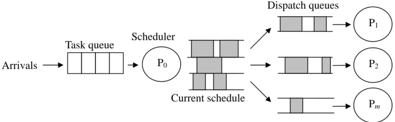
A dynamic multiprocessor system consists of m+1 processors. One of them is a dedicated scheduling processor called the system processor or scheduler, and the other m processors are application processors. In a centralized scheduling scheme, all tasks arrive at the scheduler, and distributed to application processors. The communication between the scheduler and application processors is through dispatch queues. Figure 2.1 shows the architecture of the scheduler model [5]. The Spring system is such an example [3].
The m application processors execute dispatched tasks in parallel with the scheduler which schedules the newly arriving tasks and updates the dispatch queues. Hence, the scheduling overhead does not cause uncertainty in the executions of the dispatched real-time tasks.
2.1.3 Fault model
In Primary Backup (PB) model, each task has one primary and one backup copy [4]. The backup is redundant and started only when its primary fails. Hence, for each task Ti, the
interval between arrival time (ai) and deadline (di) must be large enough so that we can
schedule two copies of Ti before its deadline without a timing overlap. Also, the two copies
P2
Pm
Arrivals
Figure 2.1 The scheduler model Current schedule
must be scheduled on different processors [4, 8].
For using the PB model, we assume that each task encounters at most one failure either due to processor or software. That is, if a primary fails, its backup will always be completed successfully. This also implies that there is at most one failure in the system at any instant of time. We also assume that failures are independent, namely, correlated failures are not considered [12].
We assume that there exist fault-detection mechanisms, such as fail-signals for detecting processor failures and acceptance tests for detecting both processor failures and software failures [4]. The failures can be transient or permanent. The scheduler will not schedule tasks to a known failed processor. Besides, in this thesis we do not deal with faults in the scheduler by assuming that there are some approaches to tolerate the faults of the scheduler.
2.2 Related work
[1-2, 4-5, 11-14]In the past decades, many heuristic algorithms have been proposed to dynamically schedule a set of real-time aperiodic tasks. In this section, we state this scheduling problem first and then discuss an important algorithm called myopic. Next, two scheduling techniques, backup overloading and backup deallocation, are introduced. The two techniques significantly improve the performance of PB-based scheduling algorithm. Then, many work extended by myopic algorithm are described, including DMA, FTMA, and DNA. RT-SADS, value-based scheduling scheme and feedback-based adaptive scheduling scheme are presented at last.
2.2.1 The heuristic dynamic scheduling problem
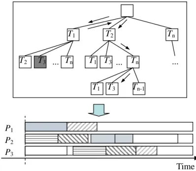
[1, 2]Scheduling a set of tasks to find a full feasible schedule is actually a search problem. The search space can be represented by a search tree. A path from the root to a leaf node
represents a scheduling sequence. An intermediate node is a partial schedule, and a leaf node is a complete schedule. A schedule is said to be feasible if all tasks in the schedule meet their deadlines. Obviously, not all leaf nodes correspond to feasible schedules. If a feasible schedule is to be found, it might cause an exhaustive search which is computationally intractable in the worst case. For the dynamic scheduling problem, heuristic approaches are taken.
Figure 2.2 depicts the concept of heuristic scheduling problem. It starts at the root of the search tree which is an empty schedule and tries to extend the schedule with one task every time. The scheduling procedure can be divided into two stages. The first is to select one task by a heuristic function. Next, after a task is selected, we use an allocation strategy for deciding when and where a task should be scheduled. In Figure 2.2, the black arrows along the tree edges indicate the extending direction and each rectangle in the feasible schedule represents scheduled task with a start time and a finish time.
Backtracking [1-5] is a branch-and bound technique. It changes the extending direction
P1 P2 P3 Time T2 Tn T2 T3 Tn T1 T3 Tn T1 ... ... ... T1 T3 Tn-1 Search space : Feasible schedule :
when the current node is not strongly-feasible. A node is said to be strongly-feasible if it is still feasible after extending it with any nodes in its next level. When backtracking, the scheduler moves back to predecessor node and uses the second highest priority task to extend the schedule until all tasks are tried.
The objective of a heuristic scheduling algorithm is to achieve higher Guarantee Ratio defined as follows [5, 11-14]:
Number of tasks whose deadline are met Guarantee Ratio =
Total number of tasks arrived in the system
×100%
2.2.2 Myopic scheduling algorithm
[1]The myopic algorithm firstly considers the real-time system with resource constraints [1]. It uses an integrated heuristic function for task selection, which captures the deadline and resource requirements of tasks. When determining the task with the minimum heuristic value and checking strongly-feasibility, it considers only the first k tasks in task queue in which tasks are maintained in the non-decreasing order of deadlines. The k is an input parameter represents the feasibility check window size. For processor allocation, it uses ASAP (As Soon As Possible) strategy. In other words, a task is assigned to a processor on which it has the earliest start time (or earliest finish time).
The termination conditions are either (1) a complete feasible schedule has been found, or (2) no more backtracking is possible. The complexity of this two-stage heuristic scheduling algorithm depends on the number of tasks in the task queue, denoted by n. Since only at most k tasks are considered, the complexity of myopic is reduced to O(kn).
The value of k can be adaptive. The larger value of k indicates more scheduling cost and usually the better scheduling result. Hence, myopic adapts the value of k based on the tightness of task deadlines and the resource contention between tasks. When the resource contention becomes serious or the deadlines become tighter, the scheduler switches k to a
PR1
BK1
larger value. This adaptation is done statically. The probability of resource contention between tasks and the average tightness of deadline of the workload have to be known in advance.
The drawback of myopic is that it does not support fault-tolerance. Besides, the value of k is difficult to be selected while we prefer a higher Guarantee Ratio rather than reducing the scheduling cost.
2.2.3 Backup overloading and backup deallocation
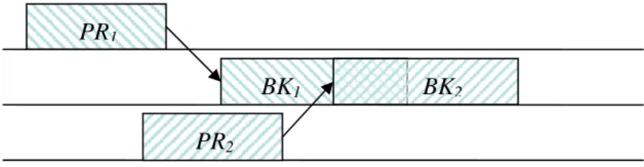
[4]Backup overloading and backup deallocation are evolved to increasing the Guarantee Ratio of those scheduling algorithms applied with the Primary Backup model. Figure 2.3 illustrates the backup overloading technique. BK1 and BK2 can overlap each other if and
only if PR1 and PR2 are scheduled on different processors. This technique saves the
computing resources reserved for redundant copies. However, the disadvantage is that it only tolerates one fault at any instant of time.
Backup deallocation is a technique which allows the scheduler to deallocate the backup when its primary is successfully completed and use the reclaimed time slots to schedule other tasks in a greedy manner [4, 5, 9]. It reduces the wasted processor time reserved for the backup copies since most of them are not executed.
2.2.4 DMA and FTMA
[5, 11]Distance Myopic Algorithm (DMA) extends the myopic algorithm with the PB-based fault-tolerant model [5]. In the DMA, the scheduler treats the primary and backup copies as
PR2
BK2
separate tasks. The primary copies are at first inserted in to the task queue in the order of non-decreasing deadlines and then the backup copies are duplicated and inserted at a fixed
distance behind their corresponding primary copies. The Fault-Tolerant Myopic Algorithm
(FTMA) further improves the way of constructing the task queue [11]. FTMA uses two task queues for the primary and backup copies separately, and blocks backup copies whose primary copies have not been scheduled outside the feasibility check window. Compared with DMA, FTMA selects more appropriate tasks to schedule. The processor allocation strategy in DMA and FTMA is the same as myopic.
Similar to myopic, FTMA and DMA have the difficulty in selecting the value of k. Moreover, DMA needs to determine one more parameter, the distance. A major disadvantage of both algorithms is that they schedule the backup copies with ASAP method which loses more opportunities to do backup overloading and deallocation. This is improved by DNA introduced below.
2.2.5 DNA
[12]The density first with minimum non-overlap scheduling algorithm (DNA) does not duplicate the tasks when constructing the task queue. Instead, it schedules two copies for each selected task in the processor allocation stage. If it cannot schedule two copies for the selected task, it rejects the task. The density function is proposed for the task selection stage, which is more complex than the integrated heuristic function used in myopic, DMA, and FTMA. The density function highlights the urgency of the tasks, and the scheduler selects the task which has the least flexibility to be scheduled. In processor allocation stage, DNA uses ASAP for allocating only the primary copies. For allocating backup copies, a minimum non-overlap strategy (MNO) is proposed for saving the available time slots of the processors. It has higher Guarantee Ratio than that of FTMA. However, the density function and the MNO strategy require higher scheduling cost.
2.2.6 Real-time self-adjusting dynamic scheduling algorithm
[2]In Real-Time Self-Adjusting Dynamic Scheduling algorithm (RT-SADS), the scheduling time has an upper bound and this upper bound can be online adjusted. The current scheduling phase will be terminated if its scheduling time reaches the upper bound. In the current scheduling phase, the scheduler adjusts the upper bound for the next one. This adaptation is based on the earliest available time of application processors and deadlines of new tasks in the task queue. The objective is to keep the application processors busy and the current length of the task queue in a reasonable range. The drawback is that RT-SADS rejects a task too late, and the system may not have enough time to handle this event of rejection.
2.2.7 Value-based scheduling scheme
[13]The value-based scheduling scheme extends the current partial schedule with multiple tasks at one time to maximize the total performance index (PI). In their scheme, the tasks have different redundancy levels and different fault probabilities. A task contributes a positive value to the PI if it is completed successfully. However, a small penalty to PI is incurred if a task is rejected and a large penalty to PI if all the copies of an accepted task failed. Hence, the more important tasks are scheduled with more copies than the less important tasks. A task can be scheduled with at most r copies, where r is the maximum redundancy level. The importance of a task depends on the value it contributes. By evaluating the expected value of the PI, the scheduler decides how many tasks are selected and how many copies are scheduled for each selected task. This algorithm takes the importance level into consideration. However, it reserves too many resources for backup copies so that the number of accepted tasks is small. Besides, the evaluation of expected value of PI requires higher complexity which is O(rk), where k is the known feasibility
check window size.
2.2.8 Feedback-based adaptive scheduling scheme
[14]The feedback-based adaptive scheduling scheme makes use of an estimation of the primary fault probability and the laxities of tasks to control the degree of overlap time between the primary copy and the backup copy of the same task [14]. This scheme allows a task to have an extremely tight deadline that is not enough for scheduling two copies with exclusive in time. When the backup copy has a timing overlap with its primary copy, parts of them are executed concurrently. If the primary copy is successfully completed, the execution of the backup copy will be terminated immediately and the remaining unused time slot will be deallocated. A modified backup overloading technique for overlapping primary with backup discussed in [15] may be applicable to this scheme. However, it is difficult to control the degree of the overlap time between the primary copy and the backup copy. Since to find a slot for a backup copy is not easy, to find a slot within a particular start and finish times is almost impossible. Besides, the effect of backup deallocation would degrade because only part of the backup copies is reclaimed.
In the next chapter, we will introduce our new effective algorithm which dynamically schedules the real-time tasks with fault-tolerance. We apply the feedback-based scheduling scheme with the loading driven adaptation strategy. When the loading exceeds the predetermined level, our algorithm begins to accept tasks without scheduling backup copies for them in order to improve the Guarantee Ratio. We also extend the waiting queue to the scheduling system which improves the utilization of the deallocated backup copy.
Chapter 3 Loading-driven Adaptive
Scheduling Algorithm (LASA)
In this chapter, we describe our new effective scheduling algorithm which monitors the system loading and controls whether it will schedule two copies for the real-time task or just one copy. In section 3.1, we give overview of our algorithm. The scheduling model with the waiting queue and the loading-driven adaptation is illustrated. In section 3.2, we describe the heuristic function used to select a task from the task queue. In section 3.3, we state the processor allocation strategies for primary and backup copies. In section 3.4, the deferment and rejection mechanism for the tasks in the waiting queue are presented. In section 3.5, we propose the loading-driven adaptation strategy for adaptive fault-tolerant scheduling.
3.1 Overview
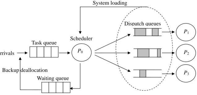
Like many previous work, our algorithm repeats two main stages until all tasks in the task queue are either accepted, rejected, or deferred. In the first stage (task selection), the scheduler selects one task by a heuristic function, and in the 2nd stage (processor allocation), the scheduler allocates primary and backup copies without timing overlap. However, there are two major differences between our algorithm and previous work. First, when the scheduler can’t find exactly two feasible slots for the selected task immediately, many existing algorithms either reject it or backtrack. However, we add a waiting queue to our system model and the scheduler moves the non-schedulable tasks to this waiting queue. Observe that perhaps a task is not schedulable right now, but it may be, later, if some previously scheduled backup copies are deallocated. Thus, when backup deallocation happens, the scheduler moves waiting tasks back to the task queue so that they will have more chances to be accepted.
Second, we proposed the loading-driven adaptation strategy which temporarily allows the scheduler to accept some tasks with allocating only the primary copies. This happens only when the system loading is heavy. Figure 3.1 depicts our scheduling model. More details are given in the following sections.
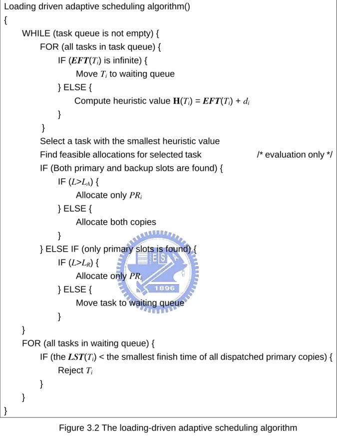
Similar to DNA [12], we don’t apply backtracking mechanism in our scheduling algorithm. As mentioned in section 2.2, there are totally n! possible paths in the search tree, where n is the number of tasks in the task queue. Each path represents a scheduling sequence and the backtracking mechanism changes to a new path when the current node is not strongly-feasible. When we need to find a fully feasible schedule for a task set, backtracking seems helpful to prevent searching the whole n! paths. But in our model the objective is to minimize number of rejected tasks, we can’t ensure that the backtracking mechanism leads searching to a better result. Besides, the backtracking mechanism increases the scheduling cost. Figure 3.2 shows the whole scheduling procedure of our algorithm. In order to describing our algorithm in some detail, we introduce the following terminology at first. P0 P1 P2 P3 Arrivals Dispatch queues Task queue Scheduler
System loading
Backup deallocation
Waiting queue
Loading driven adaptive scheduling algorithm() {
WHILE (task queue is not empty) { FOR (all tasks in task queue) {
IF (EFT(Ti) is infinite) {
Move Ti to waiting queue
} ELSE {
Compute heuristic value H(Ti) = EFT(Ti) + di
} }
Select a task with the smallest heuristic value
Find feasible allocations for selected task /* evaluation only */ IF (Both primary and backup slots are found) {
IF (L>LA) {
Allocate only PRi
} ELSE {
Allocate both copies }
} ELSE IF (only primary slots is found) { IF (L>LR) {
Allocate only PRi
} ELSE {
Move task to waiting queue }
}
FOR (all tasks in waiting queue) {
IF (the LST(Ti) < the smallest finish time of all dispatched primary copies) {
Reject Ti
} } }
Figure 3.2 The loading-driven adaptive scheduling algorithm
Definition 3.1 For a Task Ti, EFTj(Ti) is the earliest finish time of Ti executed on processor
Pj and that can complete before its deadline. If we can not find a feasible slot for Ti on Pj
EFT(Ti) = MIN{EFTj(Ti)} , for all processor Pj [11]
Definition 3.2 For a task Ti, LST(Ti) is the latest start time boundary of its primary copy.
This value is defined by the attributes of a task and is independent to the current schedule.
LST(Ti) = di -MAX{cij} – SecondMAX{cij}, for all processor Pj
Definition 3.3 For a task Ti, LFP(Ti) is the latest finish time boundary of its primary copy.
This value is defined by the attributes of a task and is independent to the current schedule.
LFP(Ti) = di – MIN{cij}, for all processor Pj [12]
In the next section, we will describe the principle of the first stage of our algorithm and the heuristic function.
3.2 The heuristic function for task selection
We use the integrated heuristic function H to select the task with smallest H value from the task queue. This function is also used in myopic, DMA, and FTMA algorithms [11].
Definition 3.4 H(Ti) is the heuristic function defined as:
H(Ti) = EFT(Ti) +di, if EFT(Ti) is not infinite.
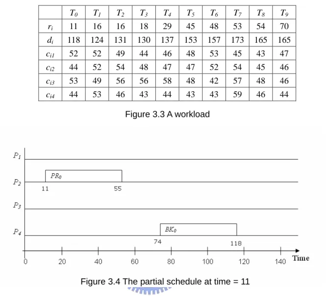
Comparing with the density function in DNA [12], we select a task which has less execution time and smaller deadline instead of which has large execution time and less scheduling flexibility selected by the density function. By this way, it can help boost the Guarantee Ratio. For example, Figure 3.3 shows a workload. Assume that there are four application processors, and the current partial schedule is shown in Figure 3.4. When T1 and
T2 just arrive at time step 16, we can calculate the heuristic values of T1 and T2 as follows.
Obviously, T1 will be selected from the task queue.
EFT(T1) = MIN{r1+c11, 55+ c12, r1+c13, r1+c14} = MIN{68, 107, 65, 69} = 65
H(T1) = EFT(T1) + d1 = 65+124 = 189
EFT(T2) = MIN{r2+c21, 55+ c22, r2+c23, r2+c24} = MIN{65, 109, 72, 62} = 62
T0 T1 T2 T3 T4 T5 T6 T7 T8 T9 ri 11 16 16 18 29 45 48 53 54 70 di 118 124 131 130 137 153 157 173 165 165 ci1 52 52 49 44 46 48 53 45 43 47 ci2 44 52 54 48 47 47 52 54 45 46 ci3 53 49 56 56 58 48 42 57 48 46 ci4 44 53 46 43 44 43 43 59 46 44 Figure 3.3 A workload
Figure 3.4 The partial schedule at time = 11
Before calculating the H value of the task, its EFT(Ti) value must be evaluated first.
The value of EFT(Ti) is not infinite means that at least one feasible slot for Ti has been
found. In our algorithm, when EFT(Ti) is infinite, Ti is moved to the waiting queue
immediately and H(Ti) needs not to be calculated.
After selecting a task from the task queue, the scheduler allocates one primary and one backup slot for it in the 2nd stage which will be described in the next section.
3.3 The processor allocation strategies
After a task Ti is selected from the task queue, the scheduler tries to allocate PRi and
BKi, which denotes the primary and backup copy of Ti, respectively. We simply use the
EFT(Ti) is found. The ASAP strategy captures both the response times and the resource
requirements of the tasks. Since a task may require different execution times on different processors, the scheduler will allocate it to the processor which can finish it with smaller response time. Meanwhile, when a processor is chosen to assign a primary copy, it must be available earlier or has less execution time for the task than other processors.
As for BKi, we allocate it by ALAP strategy. It takes more advantages of the backup
deallocation than ASAP strategy in FTMA [11]. Because the backup copies are redundant, they may not need to be executed. If a backup copy is scheduled to an earlier time slot, it possibly takes away the only chance of some other task which needs that time slot. On the other hand, when an “ASAP” backup copy is deallocated, tasks suitable for this slot may have already been scheduled to other processors or rejected. At this time, if no new tasks arrive, the deallocated slot will be wasted. In definition 3.5, we define BLST(Ti) formally,
and BKi will be allocated on the processor where this value is found.
Definition 3.5 For a task Ti, BLSTj(Ti) is the latest start time of BKi on processor Pj. If
currently there is no available time slot on Pj, BLSTj(Ti) is set as zero. We express BLST(Ti)
as follows:
BLST(Ti) = MAX{BLSTj(Ti)}, for all processor Pj, and Pj ≠ proc(PRi), where proc(PRi)
denotes the processor of PRi.
If the scheduler can’t find any feasible time slot for BKi, BLST(Ti) must be zero and
thus Ti will be moved to the waiting queue immediately. Note that when the scheduler
evaluates EFT(Ti) and BLST(Ti), it just searches for the feasible time slots. PRi and BKi are
not really allocated (dispatched). Ti will be accepted only after finding feasible time slots for
allocating both PRi and BKi.
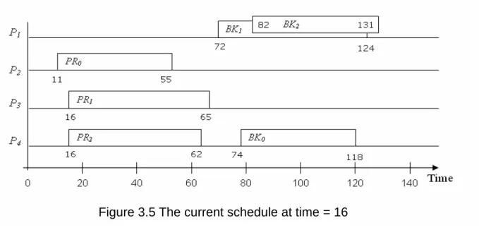
We still use the above example to illustrate our allocation strategies. After T1 is
selected, we have known that EFT(T1) = 65. Then, we find that BLST(T1) = MAX{72, 72,
the processor number. Therefore, PR1 and BK1 are allocated on P3 and P1, respectively.
After scheduling T1, the scheduler repeats these two steps and T2 is selected and scheduled
in the same way. Because the task queue becomes empty, the scheduler idles and waits for new events. Figure 3.5 shows the schedule after scheduling T1 and T2.
Figure 3.5 The current schedule at time = 16
As mentioned, when a task has an infinite EFT(Ti) or a zero BLST(Ti), it is
non-schedulable and is moved to the waiting queue. In the next section, we will describe how to maintain the tasks in the waiting queue.
3.4 Task deferment and rejection in the waiting queue
After all tasks in the task queue are processed by the scheduler and those non-schedulable tasks are moved to the waiting queue, the scheduler starts to check the tasks in the waiting queue and decide which one should be rejected. As mentioned in section 3.1, the tasks in the waiting queue will be moved back to the task queue when the backup deallocation happens. This means that a task should have enough time to wait for the next backup deallocation before its deadline. Otherwise, it should be rejected. Therefore, the scheduler has to know when backup deallocation will happen and how long a task can wait.
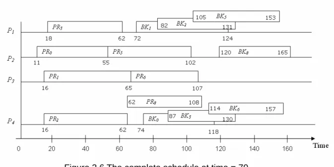
Figure 3.6 The complete schedule at time = 70
In our algorithm, we use the smallest scheduled finish time of all primary copies in the current schedule as the estimated time of the next backup deallocation. If the LST(Ti) value
is smaller than the estimated backup deallocation time, Ti is rejected. Otherwise, Ti is left in
the waiting queue.
Figure 3.6 show the complete scheduling result of above example. T4 is rejected at
time=29, because it is not schedulable and LST(T4) = 137-58-47 = 32, which is smaller than
the scheduled finish time of PR0. On the contrary, T8 is non-schedulable when it arrives at
time=54, therefore it is moved to the waiting queue. Since LST(T8) = 165-48-46 = 70,
which is larger than the scheduled finish times of PR0, PR1, and PR2, T8 is not rejected
immediately. After BK0 and BK3 are all deallocated, T8 is accepted. The Guarantee Ratio in
this example is 7/10, and finally 3 tasks are rejected.
So far, we have introduced the complete scheduling algorithm without adaptive fault-tolerance. In the next section, we will propose a mechanism which providing adaptive fault-tolerance.
3.5 The loading driven adaptation strategy
scheduler must reject some of them and tries to accept as many tasks as possible. Since rejecting the tasks incurs the system error handling routines and degrades the overall system performance, it is reasonable to intentionally stop scheduling backup copies in order to accept more tasks. Apparently, this approach takes a trade-off between the Guarantee Ratio and the degree of reliability. Hence, we propose a loading driven adaptation strategy, which aims to improve the Guarantee Ratio without sacrificing too much reliability.
Before introducing our strategy, we have to make two more assumptions. First, when the task scheduled without a backup copy fails to complete, the system error handling routines are invoked for compensating it similar to a rejected task. Second, the error handling cost for a failed is the same as for a rejected task, although the former may be a little higher.
Although the backup copies is not always necessary in our adaptive scheduling scheme, we still schedule the primary copies within the requirement: EFT(Ti) ≤ LFP(Ti), for
preserving an enough time interval between the scheduled finish time of PRi and di. This
time interval is used to make sure that in case the task is scheduled without a backup copy, the system will have more error handling time if a failure happens to the task. In other words, if a task is scheduled with only primary copy, its deadline becomes logically
LFP(Ti).
We use the average processor utilization in a small time interval to define the system loading.
Definition 3.6 Let L denotes the system loading, which is defined as:
∑
− = i i i ij a d c average m L ) ( ) ( 1, for all dispatched and not finished tasks Ti, where average(cij)
and the arrival time of T , respectively.
At the beginning, all of the dispatch queues are empty and
is the average execution time of Ti on m application processors. di and ai are the deadline i
L = 0. Then, L is increased
either successfully or faultily. Two threshold values, LA and LR, are given, so that the
scheduler switches its strategies according to the values of L, LA and LR. LA represents the
point that the scheduler starts to actively give up the feasible backup slots found for the tasks. This means that the scheduler begin to preserve processor time slots for the forthcoming tasks. However, we don’t want to accept too many tasks without finding the feasible backup slots because of reliability consideration. Only when L exceeds LR, the
scheduler accepts a task without a backup copy rather than move it to waiting queue. Intuitively, smaller threshold values results in fewer backup copies, but higher Guarantee Ratio. This is a trade-off. Notice that in our algorithm, LA can be equal to, larger, or smaller
than LR. Depending on the current value of L and the result of searching for feasible slots,
there are three cases in the processor allocation stage: Case I: Both feasible PRi and BKi slots are foun
LR
If both PRi and BKi
are possible
When L ≤ LA When L > LA
Accept Ti and allocate
and
allocate both PRi BKi
Accept Ti and
PRi only
possible Do not accept Accept Ti and a
PRi only L If only PRi is When L ≤ LR Ti When L > LR llocate LA L
Figure 3.7 The relationship among L, thresholds, and scheduling strategies
d. Ti is will be accepted. PRi will be
alloc
case, only when L > LR, the
sche
is not found. In this case, Ti is moved to the waiting queue.
ated for Ti, but BKi will be allocated only when L ≤ LA.
Case II: PRi slot is found but BKi slot is not. In this
duler accepts Ti with only PRi. Otherwise, Ti is not accepted and is moved to the
waiting queue. Figure 3.7 summarizes the relationship between the system loading and the scheduling strategies.
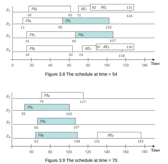
Considering the same example shown in Figure 3.3, this time we apply the adaptation strate
Figure 3.8 The schedule at time = 54
Figure 3.9 The schedule at time = 70
gy and set LA = 0.4 and LR = 0.5, in this example. When T5 arrives at time step 45, T0 ~
T4 have been scheduled and L is 0.451. Even though the scheduler finds both PR5 and BK5
slots, it only allocates PR5 because L > LA. Similarly, T6 is accepted and the scheduler
schedules only PR6. When T7 arrives at time=53, there is no available slots for it and the
scheduler moves T7 to the waiting queue. Because LST(T7) =173-59-57= 57 and the
expected nearest backup deallocation will happen at time=55, T7 is not rejected. T8 arrives at
time=54 and is moved to the waiting queue, too. Figure 3.8 shows the partial schedule at time=54.
At time=55, PR0 is finished successfully. The scheduler schedule T7 and T8 again. But
they
e=62, PR0, PR2 and PR3 are finished, and their backup are deallocated. T8 is
sche
have introduced the essence of our scheduling algorithm, including task selec
are still non-schedulable and moved to the waiting queue. T7 is rejected but T8 is still
has enough time to wait for the next backup deallocation happens at time=62, because
LST(T8)=71.
When tim
duled at time=62 with only one copy, because L is 0.448 at that time. Then T9 arrives at
time=70 and L becomes 0.319. Therefore, T9 is scheduled with two copies. Figure 3.9
shows the schedule at time=70. In this example, finally, 2 tasks are rejected and 3 tasks are accepted without backup copy. The Guarantee Ratio is 8/10, which is higher than the result generated by the algorithm without applying this adaptation mechanism (refer to Figure 3.6 in section 3.4).
So far, we
tion, processor allocation, and loading driven adaptation. In the next chapter, we will evaluate and analyze the performance of our algorithm and compare with others.
Chapter 4 Preliminary Performance
Evaluations
In this chapter, we perform a number of simulations to study the performances of our scheduling algorithm presented above. The goals of our simulations are as follows. First, we compare the overall performance of our algorithm with FTMA and DNA [11-12]. The density function is compared with EFT+D function and the MNO strategy for backup allocation is compared with ALAP [11-12]. We also want to know the effect of the waiting queue. Second, we measure the effect of the adaptive fault-tolerant scheme on Guarantee Ratio and reliability. Meanwhile, we also study the effect of threshold values of loading driven adaptation strategy. Finally, the effect of failure rate is evaluated.
4.1 Simulation overview
Our simulation program is divided into two parts, the task generator and the dynamic simulator. The task generator generates a set of real-time tasks as the input of the simulator. The dynamic simulator generates the events based on the input task set and then simulates the actions of the scheduler to the events. We will describe the details of the task generator and the simulator separately in the next two subsections.
4.1.1 The task generator
The task generator generates a set of real-time tasks in the non-decreasing order of arrival time and gives the attributes to each task according to the input parameters. The attributes, including an arrival time, a deadline, and m worst case execution times for m application processors, are generated in the following ways. For a task Ti, the worst case
parameter explanation values
MIN_C Minimum execution time 10
MAX_C Maximum execution time 80
λ Task arrival rate {0.4, 0.5,…,1.2}
R Laxity {2, 3,…, 10}
m Number of application processors {3,4,…,10} max cij 2nd max cij
R × max cij
Figure 4.1 The range of a randomly chosen deadline <The range of di>
Figure 4.2 Parameters of the task generator
The arrival time, ai, is calculated depending on the inter-arrival time between tasks, which is
exponentially distributed with mean value [5]: 2 _ _ 1 MIC C MAX C m + × × λ
, where m is the number of application processors and λ is the task arrival rate. The deadline is uniformly distributed between ai + MAX{cij} + SecondMAX{cij} and ai + R × MAX{cij},
where R is the laxity parameter which indicates the tightness of the deadline [12]. Because of the primitive of Primary Backup model, the value of R is at least 2. Figure 4.1 depicts the range for choosing the deadline. Figure 4.2 shows the input parameters used for the task generation and their possible values [12]. Thus, the task sets are generated with different combinations of above parameters for representing different workload and system scale.
parameter explanation values
FP Probability of a primary copy failure [0, 0.1]
SoftFP Probability of software failure 0.2
HardFP Probability of hardware failure 0.8
PermHardFP Probability of a permanent hardware failure 0.000001
MAX_Recovery
Maximum recovery time after a transient
hardware fault 50
Figure 4.3 Parameters for fault events
The simulator generates scheduling events and simulates the behavior of the scheduler. The events include arrival, finish, failure, and recover. The arrival events are generated according to the input task set. The finish events are generated according to the scheduling result. Failure and recover events are generated based on the parameters listed in Figure 4.3 [12]. Before generating a failure event, the simulator has to check all primary copies in the current schedule to see if they can be assigned a failure event. Because we assume that each task encounters at most one failure, the simulator do not assign a failure event to a primary copy if its backup copy overlaps with another one which has already been activated due to an earlier failure event. After all primary copies in the current schedule are checked, each eligible primary copy has the failure probability (FP) to be selected for generating a failure event. For simplicity, if more than one primary copy is selected at one time, the simulator uses the earliest one to generate a failure event. After deciding when and where a failure event happens, the simulator decides what type of this failure event is. There are three types: software failure, permanent hardware failure and transient hardware failure [5]. A software failure affects only the primary copy itself, but a hardware failure affects all primary copies scheduled on the same processor. A hardware failure can be transient or permanent. A transient hardware failure is recovered in some recovery time which is normally distributed in the interval [0, MAX_Recovery], but a permanent hardware failure will persist.
Input task set
Event generation
Event queue
Arrival ( ), Finish ( ), Failure ( ), Recover ( ), Scheduler ( )
current schedule task queue
waiting queue
parameters
Figure 4.4 The architecture of the simulator
Figure 4.4 shows the architecture of our simulator. The input data includes a task set generated by the task generator and the parameters consists of threshold values, failure probability, and feasibility check window size. The events are generated according to the input data and the current schedule. Because various events could happen at the same time, we need an event queue to order them. For every event, its corresponding function is executed. After the function is finished, the waiting queue, the task queue, and the current schedule are updated depending on the execution result.
For the comparisons among different scheduling algorithms, we have to implement different subroutines of Arrival( ), Finish( ), Recover( ), Failure( ), and Scheduler( ). The following algorithms are implemented: FTMA, DNA, New DNA (We extend a waiting queue to the original DNA), LASA (Loading-driven adaptive scheduling algorithm), and LASA’ (This algorithm is the same as LASA except that the backup allocation strategy is modified to be the MNO strategy). All these subroutines except Scheduler( ) are executed when their corresponding events happen. The Scheduler( ) is executed when task queue
becomes not empty. If more than one event happens at the same time, the execution order is: Arrival( ) → Finish( ) → Recover( ) → Failure( ) → Scheduler( ).
Two things are worthy of notice. First, both FTMA and DNA prefer to activate the scheduler periodically so that the task queue can have more tasks and then the scheduler has more choice for the task selection. If the scheduler is started immediately when the task queue becomes not empty, there is usually only one task to be considered. With only one task in the task queue to be scheduled, the heuristic function becomes somewhat useless and the task queue becomes a FIFO queue. Therefore, we periodically activate the scheduler when simulating FTMA and DNA.
Second, FTMA need the parameter, k, known as feasibility check window size. The value of k ranges from 2 to the maximum length of the task queue. Larger k usually implies higher scheduling cost, but it is not proportional to the Guarantee Ratio. Since we assume that the scheduling cost can be ignored comparing with the execution times of tasks, the value of k can be as large as possible. But the best value of k is not predictable, we test all possible k for every task set when simulating FTMA and record the best result for comparison.
4.2 Result and analysis
In this section we present the simulation results and compare the performance of our algorithm with DNA and FTMA [12, 11]. For each workload scenarios, we generate 20 task sets and each one contains 20000 independent tasks. Each data in the graph is the average of the simulations of 20 input task sets.
In the following subsections, at first, we will compare the Guarantee Ratio of various algorithms. Next, we study the reliability of the adaptive fault-tolerance and the effect of the threshold value LA and LR. At last, the effect of failure probability FP is estimated.
60.00% 65.00% 70.00% 75.00% 80.00% 85.00% 90.00% 95.00% 100.00% 0.4 0.5 0.6 0.7 0.8 0.9 1 1.1 1.2
Task arrival rate
GR FTMA DNA New DNA LASA' LASA
Figure 4.5 Effect of task load (R = 3, m = 8, FP = 0)
4.2.1 Guarantee Ratio
Figure 4.5 ~ 4.7 show the Guarantee Ratio (GR) under various task arrival rates (λ), task laxity (R), and number of processors (m). In these graphs, the GR difference between DNA and New DNA (DNA + waiting queue) is the effect of the waiting queue. The GR difference between LASA and LASA’ is the effect of ALAP and MNO backup allocation strategy.
In summary, our LASA has the highest GR compared with those of others in most circumstances, especially when the task load is heavier. In contrast, FTMA has the lowest
GR, because its major drawback is that it treats the primary copy and the backup copy as
separate tasks and allocates the backup copies by means of ASAP which let the backup copies occupy earlier processor time slots. Therefore, when the loading become heavier,
90.00% 91.00% 92.00% 93.00% 94.00% 95.00% 96.00% 97.00% 98.00% 99.00% 100.00% 2 3 4 5 6 7 8 9 10 Laxity GR FTMA DNA New DNA LASA' LASA 70.00% 75.00% 80.00% 85.00% 90.00% 95.00% 100.00% 3 4 5 6 7 8 9 10 Number of processors GR FTMA DNA New DNA LASA' LASA
Figure 4.6 Effect of laxity (λ = 0.7, m = 8, FP = 0)
Figure 4.7 Effect of number of processor (λ = 0.7, R = 3, FP = 0)
better than FTMA since it highly exploits the backup overloading and the backup deallocation. By comparing DNA and New DNA curves, we find that New DNA has higher
GR due to the effect of adding a waiting queue. We also find that ALAP strategy for
allocating backup is better than MNO used in DNA by observing that LASA has higher GR than that of LASA’ in these figures. We may conclude that backup deallocation contributes
GR more than that of backup overloading, because the MNO strategy mainly considers
backup overloading.
4.2.2 The trade-off between reliability and schedulability
We have shown the Guarantee Ratio of LASA in previous subsection. Figure 4.8 shows the average number of the primary-only tasks scheduled by LASA with various workload scenarios. When the system loading is relative low, i.e., smaller task arrival rate or larger laxity, LASA schedules fewer primary-only tasks. This result conforms to our anticipation. When the system loading is not heavy, fewer tasks are rejected and therefore the cost of executing error handling routines is low. Although we can accept them by not scheduling the backup copies, it would be better to keep the fault-tolerant capability. In (c), when the number of processors is small, there are few opportunities for backup overloading. This causes the value of L hard to exceed the thresholds. Therefore, the number of primary-only tasks is small. When the number of processor varies from 3 to 7, the number of primary-only tasks is steadily increased, but it decreased after the number of processor lager than 8. Because there are more tasks in the current schedule, the value of L becomes insensitive. This means that it will not be increased or decreased significantly after adding or removing one task from the schedule.
0 10 20 30 40 50 60 70 80 0.4 0.5 0.6 0.7 0.8 0.9 1 1.1 1.2
Task arrival rate
Number of primary-onl y tasks 0 2 4 6 8 10 12 14 16 18 2 3 4 5 6 7 8 9 10 Laxity Nu mber of primary-only tas ks 0 5 10 15 20 25 30 3 4 5 6 7 8 9 10 Number of processors N umber of p rimar y-only tas ks
Figure 4.8 Number of primary-only tasks
(a) (b)
(c)
Figure 4.9 show the GR and the percentage of primary-only tasks of our algorithm with various LA and LR. When LA and LR vary from 1 to 0, the proportion of primary-only tasks
increased from 0% to almost 100% but the improvement of GR is less than 8%. The fault-tolerant capability is highly degraded but the GR is not greatly improved when LA and
0.00% 20.00% 40.00% 60.00% 80.00% 100.00% 1 2 3 4 5 6 7 8 9 10 LA=LR GR 0.00% 20.00% 40.00% 60.00% 80.00% 100.00% Percentage of primary-only GR Percentage of primary-only 83.00% 84.00% 85.00% 86.00% 87.00% 88.00% 0.5 0.55 0.6 0.65 0.7 0.75 0.8 0.85 0.9 0.95 1 LA GR LR=0.7 LR=0.8 LR=0.9 LR=1.0
Figure 4.9 Effect of threshold values (m=8, R=3, λ=1.2, FP=0)
In Figure 4.10, we observe that LA has more influences on GR, and the difference is
about 5% when LA varies from 1.0 to 0.5. However, for any constant LA with LR varying
from 0.7 to 1.0, the difference of GR is less than 0.5%. If we don’t want to lose too much fault-tolerant capability, we should give larger values of LA and LR. Let CR and CF indicate
the average penalty caused by the rejected task and the failed primary-only task, respectively. After applying our adaptive strategy, assume that the increment of the primary-only tasks is ∆PO, and the increment of the Guarantee Ratio is ∆GR. We wish that the penalty would be reduced. In other words, ∆PO×CF×fr - ∆GR×CR ≤ 0, where fr is the
fault rate of the accepted tasks. Because we assume that CF ≅ CR, fr
PO GR ≥
∆ ∆
. If we want to make fr as large as possible, ∆GR should be very close to ∆PO. Unfortunately, ∆PO is much larger than ∆GR when LA and LR are large. In such situation, we suggest that LA and LR are
set in the interval [0.9, 1.0] for the reliability consideration.
4.2.3 The effect of failure rate
Figure 4.11 shows the effect of FP for our algorithm. We use 5 different workloads as the inputs and find that the GR decreases with the increase of FP value, especially when the task loading is heavy. In Figure 4.12, the percentage of primary-only tasks scheduled by our algorithm is shown. Here, we set LA=0.95 and LR=1.0 in order to maintain the high degree
of fault-tolerant capability for most tasks mentioned in previous subsection. When FP is larger, more backup copies are activated and fewer backup deallocations can be done. Thus,
L becomes larger and primary-only copies increased when FP is larger.
In this chapter, we have evaluated the performance of our LASA. We showed that adding a waiting queue can improve GR significantly. We also found that the adaptive fault-tolerant mechanism slightly increase the GR without losing too much fault-tolerant capability, if the threshold values are adequately given. In the next chapter, some conclusions and future work are remarked.
60.00% 65.00% 70.00% 75.00% 80.00% 85.00% 90.00% 95.00% 100.00% 0.01 0.02 0.03 0.04 0.05 0.06 0.07 0.08 0.09 0.1 FP GR (0.4, 8, 3) (1.2, 8, 3) (0.7, 3, 3) (0.7, 10, 3) (0.7, 8, 3) 0.00% 10.00% 20.00% 30.00% 40.00% 50.00% 60.00% 70.00% 80.00% 0.01 0.02 0.03 0.04 0.05 0.06 0.07 0.08 0.09 0.1 FP GR 0.00% 10.00% 20.00% 30.00% 40.00% 50.00% 60.00% 70.00% 80.00% % o f prima ry-only GR % of primary-only
Figure 4.11 Effect of failure probability on LASA. The 3-tuple means (λ, m, R), which indicating different workload scenarios.
Chapter 5 Conclusion and Future Work
In this thesis, we propose a loading driven adaptive algorithm, named LASA, which dynamically schedules real-time tasks with fault-tolerant capability based on Primary Backup model in a heterogeneous multiprocessor system effectively. Through the simulations, we have evaluated the performance of our proposed algorithm comparing with FTMA and DNA. We will make conclusions and give some future work in this chapter.
5.1 Conclusion
In summary, our new algorithm has the following main features and contributions: (1) The integrated heuristic function used for task selection in our algorithm has been shown to have the highest Guarantee Ratio than others based on our simulation results. This function selected a task which can be finished earlier and has smaller deadline.
(2) When scheduling backup copies, we have shown that ALAP strategy is the most effective strategy for cooperating with backup deallocation than ASAP and MNO strategy.
(3) By adding a waiting queue, tasks with larger deadlines have more opportunities to utilize the reclaimed backup slots when encountering heavy system loading. Thus the Guarantee Ratio is improved. Meanwhile, we use the latest start time to limit the waiting time. If a deferred task cannot be feasibly scheduled finally, it will be rejected far before its deadline so that the system still has enough time to execute error handling routines.
(4) The loading driven adaptation strategy allows the scheduler to stop scheduling backup copies temporarily when loading exceeds a predetermined threshold. Because it reduces the resources reserved for backup copies which might be unused, the Guarantee Ratio is increased with minor degradation of reliability.
5.2 Future work
In addition to our previous features, there are still some attractive issues worthy of further investigations in the future.
(1) In our task model, we assume that all tasks have the same importance. However, it will be more desirable if we allow tasks have different level of importance. More critical tasks should have higher priorities to be accepted with scheduling both primary and backup copies, even if some less important tasks must be deallocated from the current schedule. Moreover, we can schedule more than two copies for a task which has higher level of importance. In this model, how to define the importance level of tasks would be a difficult problem. It may refer to the workload of real-world applications. Besides, the performance metrics requires more sophisticated design rather than Guarantee Ratio. The importance level of individual task should be taken into consideration.
(2) We assume that each task has a large enough deadline so that primary and backup slots can be scheduled without timing overlaps. It will be more general by allowing the primary and backup copies to have timing overlaps. Even for a task with a large deadline, we can still use this approach if the only two available time slots happen to have timing overlaps. Further, if more than two copies are required for reliability, some of them should have timing overlaps. Although this scheme requires more computing resources, we can design an effective adaptation mechanism to dynamically switch the scheduling strategies.
(3) We only monitor the system loading for switching scheduling strategies, but there are still many other system statuses that may be useful. As mentioned in section 2.2, the concept of monitoring the fault rate was proposed in feedback-based adaptive scheduling scheme [14]. This can be extended to an adaptation strategy. Besides, the amount of tasks in the task queue is not considered in our algorithm. Evaluating total resource requirements of all tasks in the task queue may also be taken into consideration. We expect a more effective
adaptation strategy scheduler integrated with more than one system status, such as system loading, failure rate, and number of incoming tasks.
(4) The threshold values are constant in our algorithm. It can also be adaptive for different workload scenarios. We need a more sophisticate system model and a more complex performance metrics. As mentioned in section 4.2.2, we hope that our algorithm can still tolerate most of the failure tasks and assume that CF ≅ CR, we simply assign the LA
and LR with larger values. In the future, we may define a more precise system model in
which the tasks have different priorities, contributions and penalties. Then, we can evolve a method which dynamically adjusts the LA and LR according to the statistics of the penalty
References
[1] K. Ramamritham, J. A. Stankovic, and Perng-fei Shiah, “Efficient Scheduling Algorithms for Real-time Multiprocessor Systems”, IEEE Trans. on Parallel and
Distributed Systems, Vol. 1, No. 2, pp. 184-194, April 1990.
[2] B. Hamidzadeh and Y. Atif, ”Dynamic Scheduling of Real-time Tasks, by Assignment”, IEEE Concurrency, Vol. 6, Issue 4, pp. 14-25, Oct.- Dec. 1998.
[3] J. A. Stankovic, K. Ramamritham, “The Spring Kernel:A New Paradigm for Real-Time Systems", IEEE Trans. Software Eng., Vol. 8, Issue 3, pp. 62–72, May 1991.
[4] S. Ghosh, R. Melhem, and D. Mosse, “Fault-Tolerance Through Scheduling of Aperiodic Tasks in Hard Real-Time Multiprocessor Systems”, IEEE Trans. on
Parallel and Distributed Systems, Vol. 8, No. 3, pp. 272-284, March 1997.
[5] G. Manimaran and C. S. R. Murthy, “A Fault-Tolerant Dynamic Scheduling Algorithm for Multiprocessor Real-Time Systems and Its Analysis”, IEEE Trans. on Parallel and
Distributed Systems, Vol. 9, No. 11, pp. 1137-1152, Nov. 1998.
[6] R. Al-Omari, G. Manimaran, and A. K. Somani, “An Efficient Backup-overloading for Fault-tolerant Scheduling of Real-time Tasks”, Proc. of IEEE Workshop on
Fault-tolerant Parallel and Distributed Systems, pp. 1291-1295, 2000.
[7] R. Al-Omari, A. K. Somani, and G. Manimaran, “A New Fault-tolerant Technique for Improving Schedulability in Multiprocessor Real-time systems”, Proc. of 15th
International Parallel and Distributed Processing Symposium, April 2001.
[8] R. Al-Omari, A. K. Somani, and G. Manimaran, “Effieicnt Overloading Techniques for Primary-Backup Scheduling in Real-Time Systems” , Journal of Parallel and
Distributed Computing, Vol. 64, No. 1, pp. 629-648, Jan. 2004.