建構魚眼鏡頭反透視映射模型於障礙物偵測之應用

國 立 交 通 大 學

電機與控制工程學系

碩 士 論 文

建構魚眼鏡頭反透視映射模型

於障礙物偵測之應用

Construction of Fisheye Lens Inverse Perspective Mapping

Model and Its Application of Obstacle Detection

研 究 生：楊清泉

指導教授：林進燈 博士

建構魚眼鏡頭反透視映射模型於障礙物偵測之應用

Construction of Fisheye Lens Inverse Perspective Mapping

Model and Its Application of Obstacle Detection

研 究 生：楊清泉 Student：Ching-Chiuan Yang

指導教授：林進燈 博士

Advisor：Dr. Chin-Teng Lin

國立交通大學

電機與控制工程學系

碩士論文

A Thesis

Submitted to Department of Electrical and Control Engineering

College of Electrical Engineering

National Chiao Tung University

in Partial Fulfillment of the Requirements

for the Degree of Master

in

Electrical and Control Engineering

June 2008

Hsinchu, Taiwan, Republic of China

建構魚眼鏡頭反透視映射模型

於障礙物偵測之應用

學生：楊清泉

指導教授：林進燈 博士

國立交通大學電機與控制工程研究所

中文摘要

近年來，即使較高性能的車輛的數目有成長的趨勢，但由於輔助安全駕駛的 產品仍處於高價選購的階段而未被一般車主所接受，因此交通事故的問題仍是日 益嚴重。解決交通事故的問題可大致分為兩個部份:車輛安全系統的再提升，以及 車 主 的 安 全 駕 駛 訓 練 須 更 嚴 謹 。 本 論 文 主 要 探 討 前 者 ， 而 智 慧 型 運 輸 系 統 (Intelligent transportation system, ITS)研究其中一項即為先進車輛控制及安全系 統，世界各國研究室以及車廠均投入大量的金錢與人力來研究之，例如:日本的 Honda，Toyota，Nissan 等車廠均已研發並量產許多輔助駕駛系統。綜觀交通事故 發生的原因，主要乃是駕駛者分心所致，而主要的事故型態則以碰撞事故居多。 因此，防止碰撞即為輔助駕駛系統中一項重要的議題，本論文將採用魚眼鏡頭所 得影像為基礎並利用本文所提出的魚眼反透視映射模型將原影像經轉換後得一重 新映射之影像，並利用一般擁有垂直邊緣之物體其邊緣於重新映射後的影像之特 殊分布形式來偵測物體之所在。 在魚眼反透視映射模型的部份，我們會先指出先前研究者所提出的一般鏡頭 反透視映射方程式的謬誤，並重新提出修正後的一般鏡頭反透視映射方程式。再 加上魚眼鏡頭的模型，我們可以推導出適用於魚眼鏡頭的反透視映射模型。

在障礙物偵測的流程中，我們首先判斷影像中的動靜變化狀態，並依此狀態 選擇輪廓影像或是時間軸反透視映射差值影像其中之一作為特徵線段搜尋流程的 輸入影像。為了得到輪廓影像，我們將會執行影像銳化，邊緣偵測，形態學運算 以及修正後的細化流程等步驟。而為了得到時間軸反透視映射差值影像，我們會 對之前所得到的重新映射影像作一空間平移的動作，並與現在的重新映射影像相 減得其差值影像。在特徵線段搜尋階段後可得到一極座標直方圖，於直方圖後處 理階段將會濾除平面標線以前其他雜訊。經過追蹤和再次確認的步驟，我們可以 得知障礙物的所在位置，且若障礙物距離我們過近，系統將會發出警告以提醒駕 駛者提高警覺。 本論文所提出的障礙物偵測系統可偵測我們車輛側邊擁有垂直邊緣的物體。 此外，由於反透視映射模型的利用，我們可以估算出障礙物的所在位置且可依此 訊息做為是否警示的依據。

Construction of Fisheye Lens Inverse Perspective Mapping

Model and Its Application of Obstacle Detection

Student: Ching-Chiuan Yang

Advisor: Dr. Chin-Teng Lin

Department of Electrical and Control Engineering

National Chiao Tung University

Abstract

Due to the number of road traffic accidents is still so much even if the number of higher performance vehicle is growing up over the world in recent years. Consumers would consider not only the style and brand of vehicle but also the safety of vehicle while they are purchasing vehicles. One item of the intelligent transportation system called advanced vehicle control and safety system are focusing on the safety improvement of vehicle. Therefore, many international vehicle companies and laboratories have invested in driving safety applications, for example, Toyota, Honda, and Nissan in Japan. Most accidents result from the inattention in driving and the form of accidents is almost the collision between vehicle and other obstacles such as pedestrians, other vehicles, street light and so on. In order to avoid the collision, we develop a vision based obstacle detection system by utilizing our proposed fisheye lens inverse perspective mapping method.

In this thesis of fisheye lens inverse perspective mapping method, we point out the error which former researcher made and propose new mapping equations. After

combining the modified fisheye lens model with our modified normal lens inverse perspective mapping equations, the image captured by a fisheye lens camera can be transformed to an undistorted remapped image directly. With our normal or fisheye lens inverse perspective mapping equations, a vertical straight line in the original image will be projected to a straight line whose prolongation will pass the camera vertical projection point on the remapped image.

In this thesis of obstacle detection, we utilize the feature of object’s vertical edges to indicate the position of obstacles. We will judge the static situation of remapped image in current frame and then choose one among the profile image and temporal inverse perspective mapping difference image to be the input image of feature segments searching stage. In order to obtain the profile image, we execute sharpening, edge detection, morphological operation, and modified thinning algorithm on the remapped image. In addition, we perform a spatial shift on former frame remapped image to obtain the temporal inverse perspective mapping difference image. After feature searching stage, a polar histogram which represents the position and length of feature segment will be drawn; the histogram post-processing procedure will exclude the planar lane marking segments and noise. After tracking and confirming the obstacle candidates, the position of obstacle with respect to our vehicle will be known and stored. If the obstacle is overly approaching to our vehicle, the system will warn the driver to be attentive.

The obstacle detection system we proposed in this thesis can detect the quasi-vertical edge objects at the side of our vehicle. Moreover, the position information of obstacles can be estimated from the remapped image for further warning purpose.

致 謝

首先，在這兩年之中最為感謝的當然是我們的指導教授 林進燈教授， 這段時間以來給予我的幫助與指導，讓我學習到許多寶貴的知識與經驗，在 學業及研究方法上也受益良多。而陳永平、范剛維、蒲鶴章等口試委員們在 口試時的建議與指教，使得本論文得以更加完備，在此深感致謝。 其次，要感謝父母從小到大的辛苦栽培，女友長久以來的無悔陪伴，學 長姐的指導建議，同學的相互砥礪，學弟的認真協助。 接著要感謝清大圖書館、交大浩然圖書館以及新竹市立圖書館豐富的館 藏，讓我能夠於研究生活中增添些許知識。 謹以本論文獻給我的家人及所有關心我的師長與朋友們。

Contents

Chinese Abstract……….i English Abstract………. .. ii Chinese Acknowledgements………..v Contents………....vi List of Tables………..viii List of Figure………....ix CHAPTER 1. INTRODUCTION ... 1

1.1.BACKGROUND OF DRIVING SAFETY... 1

1.2.MOTIVATION... 3

1.3.OBJECTIVE... 5

1.4.ORGANIZATION... 6

CHAPTER 2. RELATED WORKS... 7

2.1.RELATED WORKS OF INVERSE PERSPECTIVE MAPPING (IPM) ... 7

2.2.RELATED WORKS OF FISHEYE CAMERA CALIBRATION... 8

2.3.RELATED WORKS OF OBSTACLE DETECTION... 11

CHAPTER 3. FISHEYE LENS INVERSE PERSPECTIVE MAPPING ... 13

3.1.SYSTEM OVERVIEW AND CHARACTERISTIC... 13

3.1.1. System Overview ... 13

3.1.2. System Characteristic... 14

3.2.NORMAL LENS INVERSE PERSPECTIVE MAPPING... 15

3.2.1. Brief Introduction of Normal Lens ... 15

3.2.2. Comparison with other Inverse Perspective Mapping Method... 16

3.2.3. Modified Normal Lens Inverse Perspective Mapping Method... 20

3.3.FISHEYE LENS INVERSE PERSPECTIVE MAPPING... 25

3.3.1. Brief Introduction of Fisheye Lens ... 25

3.3.2. The Fisheye Un-distortion Model ... 25

3.3.3. The Complete Fisheye Lens Inverse Perspective Mapping ... 27

CHAPTER 4. OBSTACLE DETECTION ALGORITHM ... 31

4.1.IMAGE PRE-PROCESSING... 32

4.1.1. Profile image ... 32

4.2.FEATURE SEARCHING ALGORITHM... 38

4.3.HISTOGRAM POST-PROCESSING... 42

4.4.OBJECT TRACKING,CONFIRMATION AND INFORMATION EXTRACTION... 44

CHAPTER 5. EXPERIMENTAL RESULTS... 45

5.1.RESULTS AND COMPARISON OF NORMAL LENS... 45

5.2.THE EXPERIMENTAL CONFIGURATION... 46

5.2.1. The Experimental Setup... 46

5.2.2. The Program Interface and Platform Information... 47

5.3.RESULTS OF DISTINCT ENVIRONMENT... 48

5.3.1. Results of Fisheye Lens Inverse Perspective Mapping and Obstacle Detection ... 48

5.3.2. Results of Obstacle Tracking ... 52

5.3.3. Results of Obstacle Warning ... 54

5.4.DISCUSSION... 55

CHAPTER 6. CONCLUSIONS... 57

List of Tables

Table 1: The sub-items of intelligent transportation system ... 1 Table 2: Case number of traffic accidents over the world from 1995 to 2006... 4 Table 3: The specification of platform information ... 48

List of Figures

Fig. 3-1: The overall system flow chart ... 15

Fig. 3-2: The rays pass through normal lens ... 16

Fig. 3-3: World and image coordinate system... 17

Fig. 3-4: (a) Bird’s view and (b) side view of the geometric relation between the... 17

Fig. 3-5: The vertical line projection consequence of equation (3-1) ... 19

Fig. 3-6: The wrong projection consequence of equation (3-1)... 20

Fig. 3-7: The expectative results of diagrams (a) perspective effect removing (b) a vertical straight line in the image will be projected to a straight line whose prolongation will pass the camera vertical projection point on the world surface (c) a horizontal straight line in the image will be projected to a straight line instead of an arc on the world surface. .... 21

Fig. 3-8: Geometric relation and triangulation of image coordinate system and world coordinate system which we will use in deriving process. ... 23

Fig. 3-9: The rays pass through fisheye lens... 25

Fig. 3-10: The barrel distortion ... 25

Fig. 3-11: The fisheye lens model ... 27

Fig. 3-12: The original and adjusted scope ... 28

Fig. 3-13: The (a) real scene image (b) distorted image (c) desired image ... 29

Fig. 4-1: The flow chart of image pre-processing... 32

Fig. 4-2: The unsharp mask illustration ... 33

Fig. 4-3: The results of sharpening process. (a) the blurred image (b) the sharpened image ... 33

Fig. 4-4: The results of edge detection and morphology operation ... 35

Fig. 4-5: The results of profile searching. (a) the remapped image (b) the profile image ... 36

Fig. 4-6: The idea illustrations of temporal fisheye lens inverse perspective mapping difference image. Upper: planar object patterns. Lower: non-planar object patterns ... 37

Fig. 4-7: The results of temporal fisheye lens inverse perspective mapping process. .... 38

Fig. 4-8: The result of feature searching procedure using profile image. (a)The ... 39

Fig. 4-9: The result of feature searching procedure using temporal difference ... 40

Fig. 4-10: The flow chart of feature searching... 41

Fig. 4-11: The flow chart of histogram post-processing ... 42

Fig. 4-12: The trapezoid shape histogram caused by lane markings ... 43

Fig. 4-13: The process of histogram post-processing (a) The polar histogram of ... 43

Fig. 4-14: The flow chart of object tracking, confirmation and information extraction . 44 Fig. 5-1: The results of normal lens inverse perspective mapping equations ... 46

Fig. 5-3: The program interface in the PC platform... 47

Fig. 5-4: The results of fisheye lens inverse perspective mapping and obstacle detection in different scenery... 52

Fig. 5-5: Results of obstacle tracking in Scenery 1... 53

Fig. 5-6: Results of obstacle tracking in Scenery 3... 54

Fig. 5-7: Results of obstacle warning... 55

Chapter 1. Introduction

1.1. Background of Driving Safety

The history of vehicle could be traced back to the 18th century. At that time, vehicle was a simple steam-powered three wheeler. As time goes on, there are many variations on vehicle improvement, such as the change of power, the change of style, and the change of function.

Nowadays, in addition to the consideration of vehicle style and brand, more and more consumers would take other factors into account. For example: the safety of vehicle, the entertainment equipments, the engine performance of vehicle and so on. Due to the demands of consumers, new generation vehicle which involves in the intelligent transportation system (ITS) has been developed rising and flourishing. The intelligent transportation system sub-items are listed in Table 1 [1].

Table 1: The sub-items of intelligent transportation system

Items Some sub-items

Advanced Traffic Management Systems (ATMS)

Changeable Message Sign Weigh-In-Motion

Electronic Toll Collection Automatic Vehicle Identification

Advanced Traveler Information Systems (ATIS)

Highway Advisory Radio Global Positioning System Wireless Communications Advanced Vehicle Control and Safety Systems

(AVCSS)

Collision Avoidance Systems Driver Assistance Systems Automatic Parking System Commercial Vehicle Operations

(CVO)

Automatic Cargo Identification Automatic Vehicle Location

Advanced Rural Transportation Systems

(APTS) Electronic Fare Payment

(ARTS)

Automatic Event Detection Optimal Route Guidance

The intelligent transportation system which we emphasize on advanced vehicle

can be subdivided into two parts: (1) high performance and pollution-less power (2) intelligent control and advanced safety. For high performance and pollution-less power, many engineers have developed some new fuels or power such as bio-alcohol, bio-diesel fuel, hydrogen-based power, and hybrid power. For intelligent control and advanced safety, the objective of this part is to assist drivers when they are inattentive by using sensors and controllers. There are great deals of researches that have been done in this part. For instance, pre-collision warning system, intelligent airbags, electronic stability program (ESP), adaptive cruise control (ACC), lane departure warning (LDW) and so on.

More and more international vehicle companies or groups have invested in driving safety applications, for example, Toyota, Honda, and Nissan in Japan developed many products continuously. In Europe, the PREVENT project of i2010 will research and promote this project in order to decrease the number of casualty in the traffic accidents.

For driving safety, either vision-based (passive sensor) or radar-based (active sensor) sensing system are used in the intelligent vehicle in order to help driver deal with the situations on the road. The radar-based sensing system can detect the presence of obstacle and its distance, but the drawbacks of this system are low spatial resolution and slow scanning speed. Erroneous judgment will occur when the system is lying in the complicated environment or bad weather. Although vision-based sensing system will also suffer from the environment and weather restriction, it still provide more information and real scene to drivers to see what is happened when the

system is alarming.

The vision-based sensing system used in the intelligent vehicle can be subdivide into four parts by function: (1) obstacle warning system, (2) parking-assist system, (3) lane departure warning system ,(4) interior monitoring systems [2].Within this thesis, we concern about the first and the second part only.

1.2. Motivation

In general, the objective of camera calibration is to extract the intrinsic and extrinsic parameter of camera and then use these parameters to reconstruct the three-dimension world coordinate. Nevertheless, the performance of camera calibration is affected by perspective effect, lens distortion and number of camera. An alternative method named inverse perspective mapping can be utilized to reconstruct the three-dimension world coordinate by using a camera merely. The inverse perspective mapping method using normal lens developed by Broggi had a serious error. We hope to develop an accurate fisheye lens based inverse perspective mapping method for further use.

According to the statistics [3] in Table 2, the number of higher performance vehicles is growing up over the world in recent years, but the number of road traffic accidents number which involves the fatality and injury traffic accidents is still so much. By researching the factors of them, we can refer to a main reason: improper driving, such as inattentive driving, failing to slow down, drunk driver fatigue and so on.

To analyze the type of accidents, we find out a fact that collision accidents between vehicle and other generalized obstacles occur most frequently. For example, vehicle could collide with pedestrians, collide with other vehicle, or collide with static objects. So far, researchers have proposed many methods which focus on the

avoidance of collision with front or back coming vehicles. The lateral collisions usually classify to the blind spot detection problem. But another type of lateral collision will occur when the obstacle moving direction is perpendicular to our vehicle moving direction.

There is a kind of situation that drivers or passengers alight from vehicle with carelessness. When they open the door directly without checking the nearby objects, they will collide with other pedestrians or motorcyclists or cyclists and then cause accidents. The other one is when we park our vehicle. It is because of the eyesight shelter by the vehicle body, we could not see the region of the other side of vehicle, and our vehicle will probably collided with some objects.

From above statements, we can conclude that it’s necessary and important to acquire the lateral scenery to detect the presence of obstacles while driving on the road or parking. The lateral obstacle detection system plays a significant role in improving the driving safety. Moreover, the lateral obstacle detection system could integrate with other position system such as frontal and rear obstacle detection system to become an around vehicle obstacle monitor system.

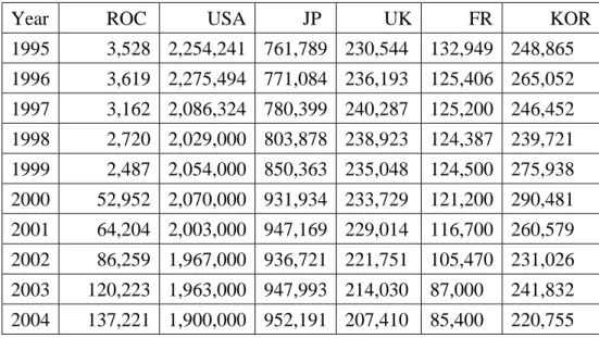
Table 2: Case number of traffic accidents over the world from 1995 to 2006

Year ROC USA JP UK FR KOR

1995 3,528 2,254,241 761,789 230,544 132,949 248,865 1996 3,619 2,275,494 771,084 236,193 125,406 265,052 1997 3,162 2,086,324 780,399 240,287 125,200 246,452 1998 2,720 2,029,000 803,878 238,923 124,387 239,721 1999 2,487 2,054,000 850,363 235,048 124,500 275,938 2000 52,952 2,070,000 931,934 233,729 121,200 290,481 2001 64,204 2,003,000 947,169 229,014 116,700 260,579 2002 86,259 1,967,000 936,721 221,751 105,470 231,026 2003 120,223 1,963,000 947,993 214,030 87,000 241,832 2004 137,221 1,900,000 952,191 207,410 85,400 220,755

2005 155,814 1,852,444 933,828 198,735 84,500 214,171 2006 160,897 - - - - -

1.3. Objective

In order to extract the three-dimension world coordinate information and modify the fault of Broggi’s inverse perspective mapping method, we will propose an accurate normal lens inverse perspective mapping method and fisheye lens inverse perspective mapping algorithm respectively.

To avoid the collision between our vehicle and other obstacles, we develop the vision-based obstacle presence and distance detection system by mounting the single fisheye camera at the midst of two lateral vehicle doors and rising out a distance from the road surface. With some intrinsic and extrinsic parameter of the camera in advance, the system will establish a transformation table to map the real road surface coordinate and the distorted image coordinate. Then the relationship of real road surface and image will be known and that will be utilized for the purpose of obstacle distance measurement.

Our obstacle detection system is focus on the detection of obstacles which have vertical edges or quasi-vertical edges. Through the phenomenon: the obstacles which have vertical edges or quasi-vertical edges in the real world, these vertical edges will transform to the radial line from a center on the transformed image. By using this characteristic, we can process the transformed image to extract the profile of edges, and then compute the polar histogram in order to post-process. After some post-processing and tracking steps, the system will find out the position of obstacles and warn driver with arising the vigilance.

1.4. Organization

This thesis is organized as follows. In Chapter 2, we will survey the related topics papers then discuss the methods and their applications, pros and cons. Chapter 3 describes the comparison with other researcher in inverse perspective mapping formula, then we will propose our modified inverse perspective mapping formula coupled with fisheye lens un-distortion formula. Next, the complete obstacle detection algorithm will be presented in Chapter 4. Chapter 5 will show the experimental results. Finally, the conclusion of our system and future works will be presented in Chapter 6.

Chapter 2. Related Works

2.1. Related Works of Inverse Perspective Mapping

(IPM)

The objective of inverse perspective mapping method is to remove the perspective effect caused by camera. This effect will cause the far scene to be condensed and always make following processing to be confused.

The main team who researched about the application of inverse perspective mapping topic are Alberto Broggi’s team at the University of Parma in Italy. First, they proposed a inverse perspective mapping theory and establish the formulas [4]. Then they use these theories combine with some image processing algorithm, stereo camera vision system, and parallel processor for image checking and analysis (PA-PRICA) system which works in single Instruction multiple data (SIMD) computer architecture to form a complete general obstacle and lane detection system called GOLD system [5]. The GOLD system which was installed on the ARGO experimental vehicle is in order to achieve the goal of automatic driving.

There are other researchers using the inverse perspective mapping method [4] or similar mapping method combining with other image processing algorithm to detect lane or obstacles. For example, J. H. Lai [6] used both of vision and ultrasonic senor on the mobile robot to detect the wall in the indoor environment. W. L. Ji [7] utilized inverse perspective mapping to get the 3D information such as the front vehicle height, distance, and lane curvature. Cerri et al. [8] utilized stabilized sub-pixel precision IPM image and time correlation to estimate the free driving space on highways. Muad et al. [9] used inverse perspective mapping method to implement lane tracking and discussed

the factors which influent IPM. Tan et al. [10] combined the inverse perspective mapping and optic flow to detect the vehicle on the lateral blind spot. Jiang et al. [11] proposed the fast inverse perspective mapping algorithm and used it to detect lanes and obstacles. Nieto et al. [12] proposed the method that stabilized inverse perspective mapping image by using vanish point estimation.

2.2. Related Works of Fisheye Camera Calibration

The wide angle camera was generally used in many applications, such as photography, surveillance system, driving assist system and so on. The reason that users adopt the wide angle camera or fisheye camera is due to capture wider scope images. The wide angle camera generally has focal length less than 35mm, or angle of view more than 60 degree. Although it has the advantage of extensive scope, the images taken from these cameras always have distortion effect such as barrel distortion or other geometric distortion. These distortions move the pixels inward or outward from the image center. If the scope has wider filed of view, the degree of distortion is more serious. As results of image deformation, many researches about the topic of distortion correction or camera calibration have been developed.

Following are some methods about distortion correction. In this thesis, we only discuss the barrel distortion caused by fisheye camera. In general, correction can be classified into two basic methods: (1) polynomial and curve fitting based method

(parametric based), (2) model and optimization based method (non-parametric based). For polynomial and curve fitting based method, the images often be corrected by

using the nonlinear optimization of the points lying on some 3D objects or planar grids. Most researchers referred to Tsai [13] who proposed the polynomial equation (2-1) to model distortion effect,

r_u =r_d(1+k₁r_d2 +k₂r_d4) (2-1) where means the distance in the undistorted image from image center to pixel, and

means the distance in the distorted image between image center and pixel, and

controls the main distortion factor, is need to be adjusted when the distortion is serious. Later researchers modified above equation to adapt their applications, such as Vass et al. [14] revised equation (2-1) to solve the shrinking, non-radial, and asymmetric problem and the result equation is show in equation (2-2),

u r d r k₁ 2 k p p (1 kp k (1 )p k (p pdy2)2) 2 dx 2 2 dy x 1 2 dx 1 dx ux = + + +λ + + and (p p ) ) s k )p (1 s k p s k (1 p p_uy = _dy + 1 _dx2 + 1 +λ_{y dy}2 + 2 _dx2 + _dy2 2 (2-2)

where means the vertical and horizontal distance in the undistorted image

between image center and pixel, and means the vertical and horizontal distance

in the distorted image from image center to pixel. controls the main distortion factor, is the secondary factor used in the border. The variable s controls the squeeze factor.

Finally uy ux,p p dy dx,p p 1 k 2 k , y x λ

λ are the asymmetric factor or called x and y curvature. But above two polynomial methods both have a drawback that is the inverse of polynomial function is difficult to be derived [15] and they could not perform well when image distortion is serious [14]. Another author Ma et al. [15] proposed series of rational polynomial functions to solve the inverse function problem and ensure these functions perform well in similar situation. But when the distortion effect is so significant, it will cost much more time and increase heavier computational complexity to estimate the distortion coefficients.

which do not perform well for serious distortion image, Devernay et al. [16] proposed a fisheye lens model which was based on the principle comonformation of fisheye lens. He observed that “ distance between an image point and the principal point is usually roughly proportional to the angle between the corresponding 3D point, the optical center, and the optical axis “. The model which called field of view (FOV) model has the distortion function pair as equation (2-3),

) 2 tan (2r tan 1 r u 1 -d ω ω = and ) 2 2tan( ) tan(r r d u ω ω = (2-3)

where r ,u rd have the same meaning as mentioned above, and ω is the only one parameter to adjust the model. Though there is only single parameter to influent this model, it is sensitive and difficult to obtain an optimal value and this model does not provides relations between the distortion parameters and the physically measurable lens parameters [17]. Pers et al. [17] proposed another fisheye lens model which has assumption as follows: “barrel distortion of wide-angle lens occurs due to the transformation of radius on the observed plane to the radius on the image plane under the influence of the viewing angle“. In other words, the view angle will cause the barrel distortion which is a radius change. By this assumption, he derived the fisheye lens distortion function as show in equation (2-4),

) f r 1 f r ln( * f r ₂ 2 u u d = + + and f r -f -2r u _d d e 1 -e * 2 f -r = (2-4) where have the same meaning as mentioned above, and the only one parameter is focal length f. Though this model links the relation of distortion parameters and the physically measurable lens parameters, it is still hard to estimate the critical parameter f which is the most important factor of the depth of filed. If higher precision is needed, above two models need to execute the feature optimization in order to obtain the best parameter values.

u

2.3. Related Works of Obstacle detection

The obstacle detection is the primary task for intelligent vehicle on the road, since the obstacle on the road can be approximately discriminated from pedestrian, vehicle, and other general obstacles such as trees, street lights and so on. The general obstacle could be defined as objects that obstruct the path or anything located on the road surface with significant height.

For pedestrian detection, many theorems have been developed, for instance, Curio et al. [18] used contour, local entropy, and binocular vision to detect the pedestrians. Bertozzi et al. [19] utilized stereo infrared camera and three approaches: warm area detection, edge based detection, and v-disparity computation to detect pedestrian and used head morphological and thermal characteristics to validate the presence of pedestrian. Though infrared cameras perform well either daytime or night, the drawback is that the cost of these cameras is still a lot.

For vehicle detection task, there are great deals of cues such as symmetry, color, shadow, corner, Vertical/horizontal edges, texture, and vehicle light [20] can be used to do this task. We will discuss some of these methods; Kyo et al. [21] used edge to detect possible vehicle and utilized symmetry, shadow underneath the vehicle, and differences in gray-level average intensity to validate the vehicle. And some other authors, for instance, Danasi et al. [22] used pattern matching to detect and validate vehicles, but this method fails when obstacle does not match the models and will loss of depth of field.

For general obstacle detection task whose definition is described as above, it can also transfer the problem to free driving space detection. Many literatures about general obstacle detection used optical flow based methods or stereo based methods. For optical

flow based methods which indirectly compute the velocity filed and detect obstacle by analyzing the difference between the expected and real velocity fields, Kruger et al. [23] combined optical flow with odometry data to detect obstacles. However, optical flow based methods have drawback of high computational complexity and fail when the relative velocity between obstacles and detector are too small. For stereo based methods, Koller et al. [24] utilized disparities in correspondence to the obstacles to detect obstacle and used Kalman filter to track obstacles. But the performance of stereo methods depends on the accuracy of identification of correspondences in the two images. In other words, searching the homogeneous points pair in some area is the prime task of stereo methods.

Chapter 3. Fisheye Lens Inverse

Perspective Mapping

3.1. System Overview and Characteristic

3.1.1. System Overview

The overall system flow chart is shown in Fig. 3-1. At the beginning, we will merely process the monochromatic information; therefore the RGB images should be transformed into 8 bits gray level images. Then, the previous established fisheye lens inverse perspective mapping table will be utilized to map the pixels from the real world road surface coordinate to the distorted image coordinate; therefore we will obtain an undistorted road surface bird’s view image after this step, and the preliminary and detailed contents will be described in Section 3.2 and Section 3.3.

While we are obtaining the bird’s view road surface image captured by the camera mounted on the vehicle side door, the flow will enter the principle obstacle detection parts of the system. After some pre-processing steps which will be described in Section 4.1, we will acquire an edge profile of bird’s view road surface image or temporal fisheye lens inverse perspective mapping difference image. Then, the segment searching algorithm will be performed on the previous obtained edge profile or a temporal difference image to get the feature radial lines which indicate the obstacles, and this algorithm will be presented in Section 4.2. After searching the feature segments, the polar histogram which represents the direction and size of obstacles will be computed. The histogram post-processing will be executed follows the obtaining of polar histogram to filter out some confusing noise or too low obstacles. Above

histogram-relative flows will demonstrate in Section 4.3. When the objects are detected by above flows, we still need to ensure the accuracy whether the objects are obstacles or not. If the obstacle passes the tracking algorithm, we will extract the relative information of the obstacle and show on the output frame. The obstacle tracking and information extraction method will be described in Section 4.4.

3.1.2. System Characteristic

The system which we developed is different in many aspects from other authors; we will list three differences below.

(1) The position of camera in our system is mounted at the midst of two side car doors and the camera captures the lateral scene in order to detect lateral obstacles. However, other authors often mounted the camera in front or in back of vehicle to detect the front or rear obstacles.

(2) Due to the position of camera, the scenes captured by camera always vary quickly on each frame; the appearance duration of obstacles maybe very short so that the difficulty of detection accuracy will increase.

(3) The property of fisheye lens camera has wider scope than normal lens camera, furthermore it accompanies the confusing distortion effect while we processing the image.

Fig. 3-1: The overall system flow chart

3.2. Normal Lens Inverse perspective mapping

3.2.1. Brief Introduction of Normal Lens

Since focal length matches the sensor format being used, a normal lens with natural filed of view does not subject to perspective distortion. The refraction angle of the image and the incident angle is nearly the same, as shown in Fig. 3-2.

Fig. 3-2: The rays pass through normal lens

3.2.2. Comparison with other Inverse Perspective Mapping

Method

The perspective effect caused by the camera view angle and distance between objects and camera often contributes to connect difference amount of information content to each pixel. In other words, we can observe that the closer distance of pixels between represent scenery object and camera is, the less information involved in the pixels is. Contrarily, the single pixel carries more information while the distance of pixels between scenery object and the camera is further. This effect always causes the non-homogenous information content distribution among all pixels.

To cope with above problem, an inverse perspective mapping transformation method will be introduced to remove perspective effect, and remap each pixel on the original camera’s image to a new position on the remapped two-dimension image. Hence we will obtain a new image whose pixels indicate homogeneous information content.

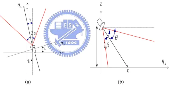
Fig. 3-3: World and image coordinate system x η y η x

η

(a) (b)

Fig. 3-4: (a) Bird’s view and (b) side view of the geometric relation between the world coordinate and image coordinate system.

Broggi et al. [4] had proposed the inverse perspective mapping method based on some prior knowledge and the flat road assumption many years ago. Though his theorem is roughly accurate, he still made an erroneous consequent in the transformation equation pair. We will point out what’s the error Broggi made later, and we list his transformation equation pair in equation (3-1) and (3-2). The spatial

relationship between the world coordinate and image coordinate system is shown in Fig. 3-3,Fig. 3-4. D ) 1 -n 2 v -sin( * ) 1 -m 2 u -cot( * H Y L ) 1 -n 2 v -cos( * ) 1 -m 2 u -cot( * H X + + + = + + + = α α γ β β θ α α γ β β θ (3-1) 1 -m 2 ) -( -) D -Y )) L -X D -Y ( sin(tan * H ( tan u 1 -1 -β β θ = 1 -n 2 ) -( -) L -X D -Y ( tan v 1 -α α γ = (3-2)

Before examining the equations, we will first introduce some notations as follows: (u,v) : The image coordinate system.

(X,Y,Z) : The world coordinate system where (X,Y,0) represent the road surface. (L,D,H) : The coordinate of camera in the world coordinate system.

θ: The camera’s tilt angle. γ : The camera’s pan angle.

β

α, : The horizontal and vertical aperture angle. m,n : The dimension of image (m by n image). O: The optic axis vector.

y x,η

η : The vector which represents the optic axis vector O projected on the road surface and its perpendicular vector.

From equation (3-1), the vertical straight line in the image coordinate system is represented by the pixels set whose v coordinate value is constant. If we assume

1 -n 2 v

-Kv=γ α + α is constant, then equation (3-1) will be transformed into equation (3-3) which is shown below.

D sin(Kv) * ) 1 -m 2 u -cot( * H Y L cos(Kv) * ) 1 -m 2 u -cot( * H X + + = + + = β β θ β β θ (3-3)

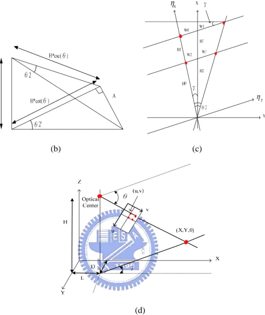
After simple computation, we can obtain the equation (3-4) from equation (3-3) and the diagram which is shown in Fig. 3-5.

X-L=(Y-D)*cot(Kv) (3-4) The meaning of equation (3-4) is that a vertical straight line in the image which represented the vertical edge of obstacle or other planar marking in the world coordinate system will be projected to a straight line whose prolongation will pass the camera vertical projection point on the world surface.

Fig. 3-5: The vertical line projection consequence of equation (3-1)

Similarly, from equation (3-1), the horizontal straight line in the image coordinate system is represented by the pixels set whose u coordinate value is a constant. If we

assume 1 -m 2 u

equation (3-5) which is shown as follows. D ) 1 -n 2 v -sin( * K D ) 1 -n 2 v -sin( * cot(Ku) * H Y L ) 1 -n 2 v -cos( * K L ) 1 -n 2 v -cos( * cot(Ku) * H X + + = + + = + + = + + = α α γ α α γ α α γ α α γ (3-5)

Thus, we can derive the equation (3-6) from equation (3-5) and obtain an unreasonable consequence which is shown in Fig. 3-6.

(X-L)2+(Y-D)2 =K2 (3-6) The meaning of equation (3-6) is that a horizontal straight line in the image will be projected to an arc on the world surface, and this result does not tally with intuition.

Fig. 3-6: The wrong projection consequence of equation (3-1)

3.2.3. Modified Normal Lens Inverse Perspective Mapping

Method

In order to modify the error mentioned in Section 3.2.2, we will propose a new transformation equation pair with two expectative results: (1) a vertical straight line in the image will still be projected to a straight line whose prolongation will pass the camera vertical projection point on the world surface, (2) a horizontal straight line in the

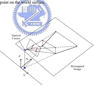
image will be projected to a straight line instead of an arc on the world surface. This result can be verified by similar triangle theorem. With some prior knowledge such as the flat road assumption and intrinsic and extrinsic parameters, we will be able to reconstruct a two-dimension image without perspective effect. The expectative results of diagrams are shown in Fig. 3-7.

(a)

(b) (c)

Fig. 3-7: The expectative results of diagrams (a) perspective effect removing (b) a vertical straight line in the image will be projected to a straight line whose prolongation will pass the camera vertical projection point on the world surface (c) a horizontal straight line in the image will be projected to a straight line instead of an arc on the

world surface.

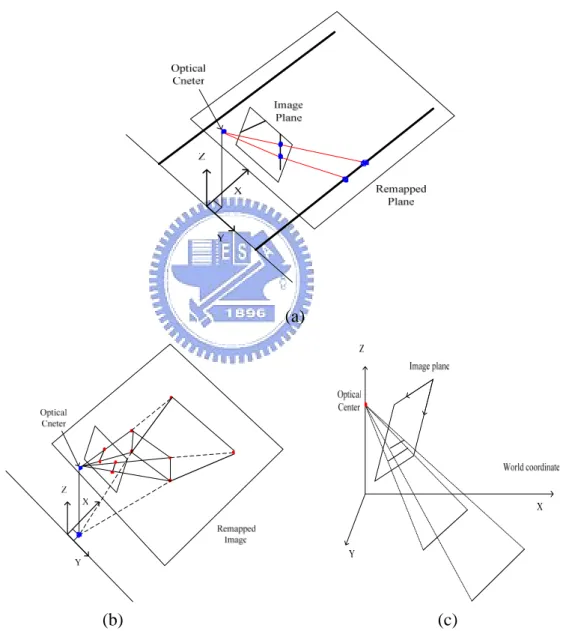
By referring to the notation mentioned in Section 3.2.2, the diagrams of relationship between image coordinate system and world coordinate system shown in Fig. 3-3,Fig. 3-4, and the illustrations of deriving process shown in Fig. 3-8, we will derive a new transformation equation pair from simple mathematical computation and triangulation.

From Fig. 3-8(a), we can obtain following equations. β β θ -1 -m 2 u 1 = → ) cot( * H H0 = θ → ) cot( * H H H₀ + ₁ = θ +θ₁ → x

η

(a)

x η y η (b) (c) (d)

Fig. 3-8: Geometric relation and triangulation of image coordinate system and world coordinate system which we will use in deriving process.

From Fig. 3-8(b), we can obtain following equations. α α θ -1 -n 2 v 2 = → ) sec( * ) tan( ) tan(θ₂' = θ₂ θ →

Finally, we combine above equations into Fig. 3-8 (c), and then we obtain the length of each segment, where each red point in Fig. 3-8 (c) represents the projection of

the red point in the first quadrant of the image coordinate system onto the road surface. Each segment length is listed as follows (Temporally assume the world coordinate of camera is (0,0,H)). ) cot( * H H₀ = θ → ) cot( * H H H₀ + ₁ = θ +θ₁ → ) sec( * H H₂ = _o γ → ) sec( * ) H (H H H₂+ ₃ = ₀+ ₁ γ → ) sec( * ) tan( * ) H (H w W₀+ ₁ = ₀+ ₁ θ₂ θ+θ₁ → ) tan( * ) H (H W₀ = ₀ + ₁ γ → ) tan( * H W₂ = ₀ γ → ) sec( * ) tan( * H W W₂+ ₃ = ₀ θ₂ θ → ) sin( * ) tan( * ) csc( * H ) cos( * ) cot( * H ) sin( * W H H X= ₂+ ₃+ ₁ γ = θ +θ₁ γ + θ +θ₁ θ₂ γ ⇒ ) cos( * ) tan( * ) csc( * H ) sin( * ) cot( * -H ) cos( * W Y= ₁ γ = θ +θ₁ γ + θ +θ₁ θ₂ γ ⇒ (3-7)

Now, we have obtained the forward transformation equations, and the backward transformation equations shown below are easily obtained by some mathematical computation. ) -) H ) sin( * Y -) cos( * X ( (cot * 2 1 -m u -1 γ γ θ β β + = ⇒ ) ) ) csc( * H ) cos( * Y ) sin( * X ( (tan * 2 1 -n v 1 1 - α θ θ γ γ α + + + = ⇒ (3-8)

To implement the inverse perspective mapping, we using the equations (3-8) instead of equations (3-7) and scanning row by row on the remapped image to compute the mapping points on the original image while we do not want an image full of hollows.

3.3. Fisheye Lens Inverse Perspective Mapping

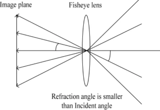
3.3.1. Brief Introduction of Fisheye Lens

Fig. 3-9: The rays pass through fisheye lens

As shown in Fig. 3-9, we can observe that the refraction angle of the image is smaller than the incident angle. Thus a fisheye lens with wider filed of view always subject to more serious perspective distortion, for example, barrel distortion as illustrated in Fig. 3-10.

Fig. 3-10: The barrel distortion

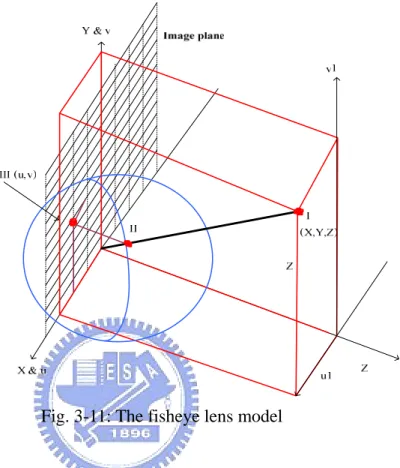
3.3.2. The Fisheye Un-distortion Model

Forster et al. [25] proposed a camera spherical projection model to implement the endoscope image formation process and utilized the warping transformation equations to correct the radial distortion. The warping transformation equation pairs and its inverse version equation pairs (3-9) and (3-10) are shown as follows. The notation of

Fig. 3-11 is listed below.

(X,Y,Z): The point in the 3D world coordinate system. (u1,v1): The coordinate in the un-distorted image (u,v): The coordinate in the distorted image. f: The focal length of camera.

R: The radius of the sphere.

v -u -R v * f Y ; v -u -R u * f X 2 2 2 2 2 2 = = (3-9) 2 2 2 2 2 2 Y X f Y * R v ; Y X f X * R u + + = + + = (3-10)

We refer to his model and modify it for our case. We can regard the X1-Y1 plane as an undistorted image plane and the u-v plane is the distorted image. Thus we can

derived the modified equations, where

R f k1 = , ) f u1 ( tan ) R u ( tan-1 -1 1 = = θ and ) f v1 ( tan ) R v ( tan-1 -1 2 = =

θ are the angle between the line connected the horizontal or vertical direction projection point of an image point with optical center and optical axis.

)) ( tan ) ( (tan -1 ) k 1 ( v v -u -R v * f v1 )) ( tan ) ( (tan -1 ) k 1 ( u v -u -R u * f u1 2 2 1 2 1 2 2 2 2 2 1 2 1 2 2 2 θ θ θ θ + = = + = = (3-11) )) ( tan ) ( (tan 1 k v1 v1 u1 f v1 * R v )) ( tan ) ( (tan 1 k u1 v1 u1 f u1 * R u 2 2 1 2 1 2 2 2 2 2 1 2 1 2 2 2 θ θ θ θ + + = + + = + + = + + = (3-12)

non-value pixels in the image. Tuning the only parameter , we can distorted or un-distorted the image whether the focal length is known or not.

1

k

Fig. 3-11: The fisheye lens model

3.3.3. The Complete Fisheye Lens Inverse Perspective

Mapping

According to the combination of the results in Section 3.2.3 and Section 3.3.2, we will propose a complete fisheye lens inverse perspective mapping algorithm. This algorithm can be divided into two sections: (1) forward mapping algorithm, (2) backward mapping algorithm. The consideration and detailed algorithm would be shown below.

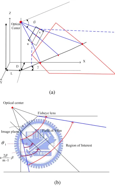
The objective of forward mapping algorithm is to search the remapped image dimensions or range. The illustration is shown in Fig. 3-12.

(a) 1 θ β β -1 -m 2 u (b)

Fig. 3-12: The original and adjusted scope

The influence factor of dimensions of scope is solely concerned with filed of view of camera whether the lens is normal lens or fisheye lens with fixed tile and pan angle. In order to reduce the confusion of computation in computing the tangent and secant triangular functions, we limit the scope of camera by condensing the filed of view. Though this action will lead to lose far and fringe information, we still retain the most scope as possible. Furthermore, we condense the angle of view by Snell’s Law like equation (3-13), where IR simulates the index of refraction and control the scope of

result range. The range of IR is between 1.3~1.7 to simulate the index of refraction of glass-based lens. ) sin( * IR ) -1 -n 2 sin(v ) sin( * IR ) -1 -m 2 sin(u 2 1 θ α α θ β β = = (3-13)

The angle θ₁andθ₂ are substituted for the equation (3-7) to compute the extreme value of X,Y coordinate value, hence we obtain the dimension of the remapped image.

The flow of backward mapping algorithm is different from forward one; it is because the backward mapping algorithm needs a radial distortion correction step. Before explaining the backward mapping algorithm, we consider to explain the idea of backward mapping algorithm by the Fig. 3-13 first.

Fig. 3-13: The (a) real scene image (b) distorted image (c) desired image

We observe that the image captured by the fisheye camera in Fig. 3-13(a) which has perspective effect and distortion simultaneously. After the inverse perspective mapping, we can expect to obtain the Fig. 3-13(b) whose perspective effect has been removed. On the image Fig. 3-13(c), the perspective effect and distortion are completely removed. By following the sequences of Fig. 3-13(a),(b),(c), we can derived a backward mapping algorithm.

First of all, we modify the equation (3-8) to equation (3-14). ) ) sin( * (IR sin * 2 1 -m u ; -) H ) sin( * Y -) cos( * X ( cot-1 -1 ₁ 1 θ β θ β γ γ θ = = + ) ) sin( * (IR sin * 2 1 -n v ; ) ) csc( * H ) cos( * Y ) sin( * X ( tan 2 1 -1 1 -2 _{θ θ} α _α θ α γ γ θ + = + + + = (3-14)

Then, we utilize the angle θ₁andθ₂ directly and equation (3-12) to perform the distortion correction. By tuning the parameter of IR and , we will finally obtain the undistorted and perspective effect removed image.

1

Chapter 4.

Obstacle Detection Algorithm

Broggi et al. [5] utilized his inverse perspective mapping method and stereo cameras to detect obstacles in front of vehicle. The left and right images captured by the camera at corresponding positions were differenced to obtain a difference image. In that image, the planar objects such as lane markings were eliminated and prominent objects were reserved as quasi-triangle pairs. By detecting these quasi-triangle pairs, the position of obstacles could be found. Nevertheless, the performance of Broggi’s detection method was obviously dependent on the obstacle height, width, distance and shape.

In this chapter, we develop an obstacle detection algorithm using spatial and temporal fisheye lens inverse perspective mapping method. We use the fisheye lens inverse perspective mapping method mentioned in Section 3.3 and single fisheye camera to detect obstacles by the side of vehicle. The definition of obstacle in this thesis excludes objects whose height shorter than a threshold and objects whose edges are not quasi-vertical. The image preprocessing process that selects a proper pattern image as the input to the feature searching procedure will be described in Section 4.1. As mentioned in Section 3.2.3, a vertical straight line in the image which represented the vertical edge of obstacle in the world coordinate system is projected to a straight line whose prolongation will pass the camera vertical projection point on the world surface. The algorithm of searching features whose definition is described above will be presented in Section 4.2. Histogram relative procedure and object tracking and information extraction are described in Section 4.3 and 4.4 respectively.

4.1. Image pre-processing

Fig. 4-1: The flow chart of image pre-processing

Since we have obtained the perspective effect removed and distortion corrected image from the fisheye lens inverse perspective mapping step, we will execute some preprocessing to extract the simplified pattern image for further process. At first, the remapped image will be smoothed by mean filter in order to reduce the noise caused from the process of image capturing and fisheye lens inverse perspective mapping transformation; hence we will obtain a blurred remapped image. After above step, we will judge the variation situation in the image by differencing the previous frame and current frame. If the objects in the world and our camera are motionless relatively, the difference image will be empty. Then we will utilize the profile image to extract the feature segments; otherwise we will use the obstacle-sensitive temporal fisheye lens inverse perspective mapping difference image to extract the features. We will discuss the flows of obtaining the profile image and temporal fisheye lens inverse perspective mapping difference image in Section 4.1.1 and Section 4.1.2 respectively.

4.1.1. Profile image

In order to extract the profile of image, we need the obvious edges of obstacles. Nevertheless, the image has been blurred by mean filter, some edges become

unapparent, thus we should emphasize the edges once again by the unsharp mask. The diagram of unsharp mask is shown in Fig. 4-2.

Fig. 4-2: The unsharp mask illustration

In Fig. 4-2, we can observe that a sharp edge E is smoothed to form the edge A, and then we will perform mean filter to smooth the blurred edge again to form the edge B. The difference of edge A and B will be done and added to the original blurred edge A, thus an obvious edge A+(A-B) will appear in the image. The result of sharpening process is shown in Fig. 4-3.

(a) (b)

Fig. 4-3: The results of sharpening process. (a) the blurred image (b) the sharpened image

An edge detection process will be operated after the sharpening stage, Gx and Gy stand for the horizontal and vertical direction 3 by 3 Sobel edge mask respectively. It

will be performed on the edge-sharpened image. Equation (4-1) show the spatial illustration and mathematic operation of Sobel edge detection,

1)] -y 1, f(x 1) -y 2f(x, 1) -y 1, -[f(x -1)] y 1, f(x 1) y 2f(x, 1) y 1, -[f(x Gx = + + + + + + + + + 1)] y 1, f(x y) 1, 2f(x 1) -y 1, [f(x -1)] y 1, -f(x y) 1, -2f(x 1) -y 1, -[f(x Gy= + + + + + + + + + (4-1) -1 -2 -1 0 0 0 1 2 1 1 0 -1 2 0 -2 1 0 -1

where the x, y is the coordinate of each pixel in the horizontal and vertical axis, and f(x,y) is the intensity of this pixel.

After detecting the edges of the remapped image, a threshold will be performed on the image in order to obtain a binary image. However the edges may not be continuous, therefore we should execute the morphological dilation and erosion process to connect these edges and discard the edges which maybe caused by noise. Equation (4-2) shows the spatial relationship and mathematic operation of morphological dilation and erosion,

X0 X1 X2 X3 X4 X5 X6 X7 X8 X8) X7 X6 X5 X3 X2 X1 (X0 X4 D= ∪ ∪ ∪ ∪ ∪ ∪ ∪ ∪ X8) X7 X6 X5 X3 X2 X1 (X0 X4 E= ∩ ∩ ∩ ∩ ∩ ∩ ∩ ∩ (4-2) Gx Gy

where the D and E are the notation of dilation and erosion value of a 3 by 3 region in a binary image. The results of edge detection and morphology operation are shown in Fig. 4-4.

Fig. 4-4: The results of edge detection and morphology operation

To extract the feature segments, we should execute the thinning algorithm [26] to thin these binary edges. However, the computational load of thinning algorithm is so huge; we perform this algorithm in another form alternatively. The modified thinning algorithm (single direction) is listed as follows.

N(x4)= x2+x3+x4+x5+x6+x7+x8+x9

S(x4) is the number of value changing of the cycle from x2,x3,x4 to x8,x9,x2

If x9 x2 x3 x8 x1 x4 x7 x6 x5 2<=N(x1)<=6 AND S(x1)=1 AND x2∩x4∩x6=0 AND x4∩x6∩x8=0 THEN x1=1

N(x1)<2 means that x1 is an end point or N(x1)>6 means that x1 is an inner point, thus we should not delete x1. S(x1)>1 stands for that x1 is a bridge point, therefore we should not erase x1 as well. The original algorithm will delete the x1 (x1=0) to thin the pattern while above conditions are satisfied, and execute this algorithm until the pattern was unit size. Contrarily, we set x1=1 to extract the exterior profile of a pattern and perform the algorithm once. Fig. 4-5 shows the result of profile searching.

(a) (b)

Fig. 4-5: The results of profile searching. (a) the remapped image (b) the profile image

After the profile searching stage, we obtain the profile image for further use. Although the results of segment searching on the profile image is not so good as the results of segment searching on the skeleton-like image, we can add some processes described later to increase the effect of segment searching.

4.1.2. Temporal fisheye lens inverse perspective mapping

difference image

The objective of temporal fisheye lens inverse perspective mapping difference process is that we would like to simulate the function of stereo vision. The advantages of stereo inverse perspective mapping are that the planar object patterns in the image could be removed by differencing the left and right remapped image and the non-planar object patterns would be reserved.

Fig. 4-6: The idea illustrations of temporal fisheye lens inverse perspective mapping difference image. Upper: planar object patterns. Lower: non-planar object patterns

According to stereo inverse perspective mapping method [5], two cameras were set apart from a distance to acquire enough overlapped information. If we would like to simulate the stereo effect by using a single camera, we need to capture the image apart from a time interval. From Fig. 4-6, there are important issues need to solve, such as the choice of time interval and the shift displacement of the remapped image. The time interval must be moderate, too long interval will produce too large region and make detection error; conversely, too short interval will produce unapparent region and bring about difficulty of obstacle detection. Similarly, the shift displacement of previous remapped image controls the coincidence of planar object patterns.

Since the moderate time interval are decided by experiential adjusting, we can compute some feature points displacement in this two remapped images and take the average displacement into the shift displacement of temporal fisheye lens inverse perspective mapping method. After thresholding process, we will obtain a stereo effect-like binary difference image for further use.

(a) (b)

Fig. 4-7: The results of temporal fisheye lens inverse perspective mapping process. (a) the remapped image (b) the temporal difference image

4.2. Feature Searching algorithm

As mentioned at the beginning of this chapter, the features we would like to search are merely the segments in the remapped image which represent the quasi-vertical edge of objects in the world coordinate system. Due to these feature segments prolongation will pass through the camera vertical projection point, we will develop a searching algorithm and scan the polar histogram.

Starting from the camera vertical projection point defined as CP on the remapped image, we scan angle by angle and scan radius outward for each angle on the pattern image such as profile and difference image from last step. In order to reduce the loss of segment points, we use a mask and set a voting threshold to search the points satisfied

with the pixel value and between distance conditions. For each angle, a segment will be output as long as its length is long enough; next segment starting point at the same angle must be close enough to the last segment in order that we merely concerned about the segment closet to CP. After searching and highlighting the segment points at each angle, we can obtain the number of segment points at the same time. These point number at each angle will be used to produce a polar histogram for further process. Some results of feature searching procedure are show in Fig. 4-8 and Fig. 4-9.The complete flow chart of feature searching is shown in Fig. 4-10.

(a) (b)

(c) (d)

Fig. 4-8: The result of feature searching procedure using profile image. (a)The sharpened remapped image, (b)The profile image, (c)The scanned feature

segments, (d)The scanned feature segments superposed on the sharpened remapped image

(a) (b)

(c) (d)

Fig. 4-9: The result of feature searching procedure using temporal difference fisheye lens inverse perspective mapping image.(a)The remapped image, (b)The temporal difference fisheye lens inverse perspective mapping image, (c)The scanned feature segments, (d)The scanned feature segments superposed on the remapped image

4.3. Histogram Post-processing

Fig. 4-11: The flow chart of histogram post-processing

As we have obtained the polar histogram of feature segments, we still need some procedure to eliminate the histogram we are not concerned, such as the planar object segment and noise segment. Due to the imperfectness of planar object segments reduction in the pattern image obtaining procedure, planar object segments will still appear and be computed at the polar histogram step. In this thesis, we barely define the lane marking as the planar object. By observing the polar histogram, we can discover that the trapezoid shape of these histogram columns means the planar objects and then delete them. To avoid the noise histogram columns, we reject the too short columns.

After eliminating planar objects and noise, we will search the local maximum position which represents the non-planar object segment position in the polar histogram. In order to reduce the confusion of too many obstacles appearing in a frame simultaneously, we pick a peak column merely at an angular interval. Now, we obtain the positions of obstacle candidates and then entry the tracking process to confirm them. Some results of histogram post-processing procedure are show in Fig. 4-12 and Fig. 4-13.

Fig. 4-12: The trapezoid shape histogram caused by lane markings

(a) (b)

(c)

Fig. 4-13: The process of histogram post-processing (a) The polar histogram of Fig.4-9, (b) The histogram of (a) after the trapezoid shape histogram elimination, low singleton histogram elimination and peak searching procedure, (c) Local peak histogram

4.4. Object Tracking, Confirmation and Information

Extraction

Local Peak Histogram Array Segment Tracking Tracked Times >Theshold No Point out Obstacles Position Planar object Judgement No Yes Point out Planar object Position Yes

Fig. 4-14: The flow chart of object tracking, confirmation and information extraction

The objective of tracking procedure is to confirm and improve the correctness of object we have detected. We choose the displacement and angle variation of feature segment on the image to be the judgment conditions, then we can track the feature segment continuously. If the feature segment passes the tracking procedure, we will judge whether this feature segment belongs to the planar object or not once more by simple pattern matching. The pattern represents the planar object is shown in Fig. 4-14. After the tracking and confirmation procedure, we can sure the feature segment we have detected is an obstacle segment and then point out the position of feature segment. Thus we will extract and store the relative information for system further use.

Chapter 5. Experimental Results

5.1. Results and Comparison of Normal Lens

Inverse Perspective Mapping Method

In section 3.2.3, we proposed a modified forward and backward normal lens inverse perspective mapping equation pairs. In order to discriminate the results, we will show the experimental results of Broggi’s equations and our equations in Fig. 5-1 with normal lens camera. The experimental environment is indoor space and the image contents are square tiles and some objects.

(a)

(c)

Fig. 5-1: The results of normal lens inverse perspective mapping equations (a) original captured image (b) bird’s view image using Broggi’s equations (c) bird’s view image using our equations

From Fig. 5-1, we note that the image captured by normal lens camera is accurately transformed to the bird’s view image by using our equations. The perspective effect in the original image leads the prolongation of vertical straight lines in the world to intersect a point called vanish point. In Fig. 5-1(b) and (c), we can observe the perspective effect is eliminated by both of Broggi’s and our equations. Nevertheless, a horizontal straight line in the world will be transformed to an arc by implementing Broggi’s equations as shown in Fig. 5-1(b). With our modified equations, a horizontal straight line in the world will still be transformed to a horizontal straight line as shown in Fig. 5-1(c).

5.2. The Experimental Configuration

5.2.1. The Experimental Setup

Without losing the generality and experimental convenience to detect the obstacles at the side of vehicle, we mounted a fisheye lens camera at the central position of two

side doors with an appropriate height. The illustration is shown in Fig. 5-2.

Fig. 5-2: The setup diagram of camera.

In order to avoid the disorder of a frame, we will merely detect the objects whose heights are more than a threshold and whose edges are quasi-vertical. The objects such as sidewalk, small balls and so on are excluded in our detection system. The experimental environment is constrained to the brighter environment and the speed of vehicle should not too fast so that the objects in frames would not move too quickly.

5.2.2. The Program Interface and Platform Information

(D) (E)

(C) (B)

(A)

Fig. 5-3 shows the program interface in the PC platform. Block (A) shows the input frame which is added the rectangle and line to indicate the position of obstacles. Block (B) contains the video relative information. Block (C) contains the extrinsic and intrinsic parameter of camera and fisheye lens inverse perspective mapping look up table production. Block (D) shows the image we used in the obstacle detection algorithm. The upper image is the remapped image which is added the rectangle and line to indicate the position of feature segments. The central image is the judgment image to judge the static situation as described in Section 4.1, and the lower image shows the input image to feature segment searching stage. Block (E) shows the histogram we have described in Section 4.3. The detailed platform information is listed in Table 3.

Table 3: The specification of platform information

CPU Intel Core Duo T2050 1.6GHz

Memory 1GB DDR2 RAM

Programming Tool Borland C++ Builder 6.0 Operation System Microsoft Windows XP Video Resolution 640x480

Frame Rate 30fps

5.3. Results of Distinct Environment

5.3.1. Results of Fisheye Lens Inverse Perspective Mapping

and Obstacle Detection

As shown in Fig. 5-4, we detected larger obstacles whose edges are quasi-vertical at the lateral side of our vehicle by using fisheye lens inverse perspective mapping method described in Section 3.3 and obstacle detection algorithm in Chapter 4. For

instance, bicyclist, street light, railings, vehicles, pedestrian and so on are detected accurately by our system.

(a) Scenery1: bicyclist, street light.

(e) Scenery 5: multiple vehicles.

Fig. 5-4: The results of fisheye lens inverse perspective mapping and obstacle detection in different scenery

5.3.2. Results of Obstacle Tracking

Since we have detected the obstacle in a frame, we should track this obstacle in successive frames continuously by checking the displacement and angular shift in the image as demonstrated in Section 4.4. The successive tracking results are shown in Fig. 5-5 and Fig. 5-6.

# Frame 314 # Frame 318

# Frame 322 # Frame 326

Fig. 5-5: Results of obstacle tracking in Scenery 1

# Frame 204 # Frame 220 Fig. 5-6: Results of obstacle tracking in Scenery 3

5.3.3. Results of Obstacle Warning

Thanks to the fisheye lens inverse perspective mapping method, the three-dimension world coordinate value could be estimated from the remapped image. In other words, when we detected the obstacle in the remapped image, we could also estimate the position information. If the obstacle is so overly approaching our vehicle exceeding a threshold, that system will alert us by arresting markings.

(b)

Fig. 5-7: Results of obstacle warning

5.4. Discussion

Though the performance of our obstacle detection system based on fisheye lens inverse perspective mapping method is satisfying, it is still subject to some disturbance factors as shown below. In Fig. 5-8 (a), the street light in the remapped image becomes unapparent due to the texture of remapped grassland behind it.

(b)

Fig. 5-8: Some example of detecting error in our system

In addition, the completeness of obstacle shape in the profile or temporal fisheye lens inverse perspective mapping difference image is critical for following obstacle detection process. Fig. 5-8 (b) show the broken shape of obstacle in the temporal fisheye lens inverse perspective mapping difference image. The broken shape will make the loss of detection.