國
立
交
通
大
學
電控工程研究所
博
士
論
文
基於模糊線性區別分析之模糊分群法與結合空間
資訊之支撐向量機
A Clustering Algorithm Based on Fuzzy-Type Linear
Discriminant Analysis and
Spatial-Contextual Support Vector Machines
研 究 生:李政軒
指導教授:林進燈 教授
基於模糊線性區別分析之模糊分群法
與結合空間資訊之支撐向量機
A Clustering Algorithm Based on Fuzzy-Type Linear
Discriminant Analysis and
Spatial-Contextual Support Vector Machines
研 究 生:李政軒 Student: Cheng-Hsuan Li 指導教授:林進燈 Advisor: Chin-Teng Lin
國 立 交 通 大 學 電控工程研究所
博 士 論 文
A Thesis
Submitted to the Institute of Electrical Control Engineering College of Electrical and Computer Engineering
National Chiao Tung University in partial Fulfillment of the Requirements
for the Degree of Doctor
in
Electrical and Computer Engineering January 2012
Hsinchu, Taiwan, Republic of China
i 基於模糊線性區別分析之模糊分群法與結合空間資訊之支撐向量機 學生:李政軒 指導教授:林進燈 博士 Chinese abstract 國立交通大學電控工程研究所博士班 摘 要 統計學習演算法自動利用觀察資料來辨識複雜的樣本並進行決策。統 計學習領域中有兩大主要議題:叢集分析與分類器設計。叢集分析演 算法會將相似的樣本組織成同一個叢集;分類器則會利用現有的訓練 樣本來決定新的未知樣本之類別。在本論文中,將提出模糊的分群演 算法與融合空間資訊的分類器。在分群演算法方面,本文提出模糊線 性區別分析之組間與組內分散矩陣,再搭配 Fisher 準則進行分群,此 方法同時最小化群內資訊與最大化組間資訊。針對分類器的部分,透 過空間資訊來調整支撐向量機的決策函數與限制式。利用真實資料的 實驗結果顯示,本論文提出的方法可以有效地增加分群與分類的效 能。
ii
A Clustering Algorithm Based on Fuzzy-Type Linear Discriminant Analysis and Spatial-Contextual Support Vector Machines
English abstract
Student: Cheng-Hsuan Li Advisors: Dr. Chin-Teng Lin
Institute of Electrical Control Engineering National Chiao Tung University
ABSTRACT
Statistical learning is trying to develop computer algorithms to recognize complex patterns and make decisions based on empirical data automatically. Two major issues are clustering and classification. Clustering organizes patterns into sensible clusters for patterns in the same cluster to be similar in a sense, whereas classification identifies the categories to which new patterns belong based on an available training set of data containing patterns of known categories. This thesis introduces a fuzzy-based clustering and a spatial-contextual classifier. Fuzzy-based clustering defines within- and between-cluster scatter matrices of a fuzzy-type linear discriminant analysis, and the clustering results are based on the Fisher criterion. The proposed clustering algorithm minimizes the within-cluster information and simultaneously maximizes the between-cluster information. For the classification part, a spatial-contextual term was used to modify the decision function and constraints of a support vector machine. Experimental results show that the proposed methods achieve good clustering and classification performance on famous real data sets.
誌
謝
Acknowledgement 首先誠摯的感謝指導教授林進燈博士、張志永博士與臺中教育大學 教育測驗統計研究所郭伯臣博士,三位老師悉心的教導使我得以一窺 特徵萃取、分群與分類等統計學習演算法領域的深奧,不時的討論並 指點我正確的方向,使我在這些年中獲益匪淺。老師對學問的嚴謹更 是我輩學習的典範。 四年半的日子裡,在工作上歷經逢甲大學應用數學系短期專任講 師、臺中教育大學教育測驗統計研究所的行政助理,在生活上歷經結 婚生子,變化頗大。但最令人懷念的是在實驗室裡共同的生活點滴, 學術上的討論,撰寫論文的革命情感。感謝立偉學長於就學期間,不 厭其煩的為我解惑,也感謝同學勝智在修課方面的幫忙,總是能帶來 課堂與所務的第一手消息。實驗室的鈞翔、志勝、士勛等學弟妹們當 然也不能忘記,你們的幫忙我銘感在心。 老婆省華在背後的默默支持更是我前進的動力,沒有省華的體諒、 包容,相信這兩年的生活將是很不一樣的光景。女兒沛芩的笑容,是 最後一個學期生活上最棒的潤滑劑,總能在我忙碌的工作之餘,放鬆 我的心情,讓我能夠重啟熱情迎接每一忙碌的日子。 最後,謹以此文獻給我摯愛的父親、母親與媽咪。
Contents
Contents Chinese abstract ... i English abstract ... ii Acknowledgement ... iii Contents ... iv List of tables ... viList of figures ... viii
List of symbols ... xii
1. Introduction ... 1
2. Literature Review of Fuzzy-based Clustering Algorithms ... 10
2.1 Fuzzy C-means Clustering Algorithm ... 10
2.2 Gustafson-Kessel algorithm ... 11
2.3 Fuzzy Compactness and Separation ... 13
2.4 Other FCM-type Clustering Algorithms ... 15
3. LDA-based Clustering Algorithm ... 16
3.1 Review of LDA ... 16
3.2 FLDC Algorithm... 17
3.3 Experiments ... 20
3.3.1 Experimental Data and Designs ... 20
3.3.2 Experimental Results ... 23
4. The Support Vector Machine and Its Spectral-Spatial Classification Schemes ... 34
4.2 Spectral-Spatial Classification Scheme Based on Partitional
Clustering Techniques ... 37
4.3 Context-Sensitive Semi-supervised SVM ... 40
5. Spatial-Contextual Support Vector Machines ... 43
5.1 A Spatial-contextual Support Vector Machine in the Original Space ... 43
5.2 A Spatial-Contextual Support Vector Machine in the Feature Space ... 49
5.3 Classification System of SCSVM and SCSVMF ... 50
5.4 Experiments ... 52
5.4.1 Experimental Data and Designs ... 52
5.4.2 Experimental Results ... 56
6. Conclusion ... 75
List of tables List of tables
Table 1 Descriptions of Three Real Data Sets ... 23
Table 2 The Mean, Standard Deviation, Maximum, and Minimum Accuracy of Clustering for Three Real Data sets. ... 33
Table 3 The Mean, Standard Deviation, Maximum, and Minimum Accuracy of Clustering for Three Real Data sets of FMSFA, Where LD Represents the Latent Dimension ... 33
Table 4 Sixteen Categories and Corresponding Number of Pixels in the Indian Pine Site Image ... 53
Table 5 The Overall Accuracies in Percentages of SCSVM (OAA, M), SCSVM (OAO, M), SCSVMF (OAA, M), and SCSVMF (OAO, M) with Different Parameters M, the Size of the Neighborhood System, and in the IPS Data set. ... 58
Table 6 The Overall Accuracies, Kappa Coefficients, and Average Accuracies in Percentages of the Experimental Classifiers for the IPS Data set ... 58
Table 7 The Class-specific Accuracies in Percentages for the IPS Data set ... 59
Table 8 The Overall Accuracies in Percentages of SCSVM (OAA, M), SCSVM (OAO, M), SCSVMF (OAA, M), and SCSVMF (OAO, M) with Different Parameters M, the Size of the Neighborhood System, and in Washington D.C. Mall Data set (Case 1). ... 64
Table 9 The Overall Accuracies in Percentages of SCSVM (OAA, M), SCSVM (OAO, M), SCSVMF (OAA, M), and SCSVMF (OAO, M) with Different Parameters M, the Size of the Neighborhood System, and in Washington D.C. Mall Data set (Case 2). ... 66
Table 10 The Overall Accuracies in Percentages of SCSVM (OAA, M), SCSVM (OAO, M), SCSVMF (OAA, M), and SCSVMF (OAO, M) with Different Parameters M, the Size of the Neighborhood System, and in Washington D.C. Mall Data set (Case 3). ... 67
Table 11 The Overall Accuracies, Kappa Coefficients, and Average Accuracies in Percentages of the Experimental Classifiers for the Washington D.C. Mall Data set (Case1). ... 68
Table 12 The Class-Specific Accuracies in Percentages for the Washington D.C. Mall Data set in Case 1 ... 68
Table 13 The Overall Accuracies, Kappa Coefficients, and Average Accuracies in Percentages of the Experimental Classifiers for the Washington D.C. Mall Data set (Case 2). ... 68
Table 14 The Class-Specific Accuracies in Percentages for the Washington D.C. Mall Data set in Case 2. ... 69
Table 15 The Overall Accuracies, Kappa Coefficients, and Average Accuracies in Percentages of the Experimental Classifiers for the Washington D.C. Mall Data set (Case 3). ... 69
Table 16 The Class-Specific Accuracies in Percentages for the Washington D.C. Mall Data set in Case 3 ... 70
List of figures List of figures
Figure 1. The spectral values obtained from the Indian Pine Site data set. The purple represents the Soybeans-min till patterns and the yellow represents the Corn-no till patterns. These two classes have similar spectral properties. ... 5
Figure 2. The support vector machine (SVM) classification results of the Indian Pine Site image, containing speckle-like errors. ... 6
Figure 3. (a) The “x” remarks 50 random samples chosen from the multivariate normal distribution with mean [0.5,0]T and covariance
8 . 0 7 . 0 7 . 0 8 . 0
, and the “o” remarks 50 random samples chosen from the multivariate normal distribution with mean [0.5,0]T and covariance
8 . 0 7 . 0 7 . 0 8 . 0
; (b) The clustering results of (a) applying FCM; (c) the clustering results of (a) applying GK algorithm. ... 12
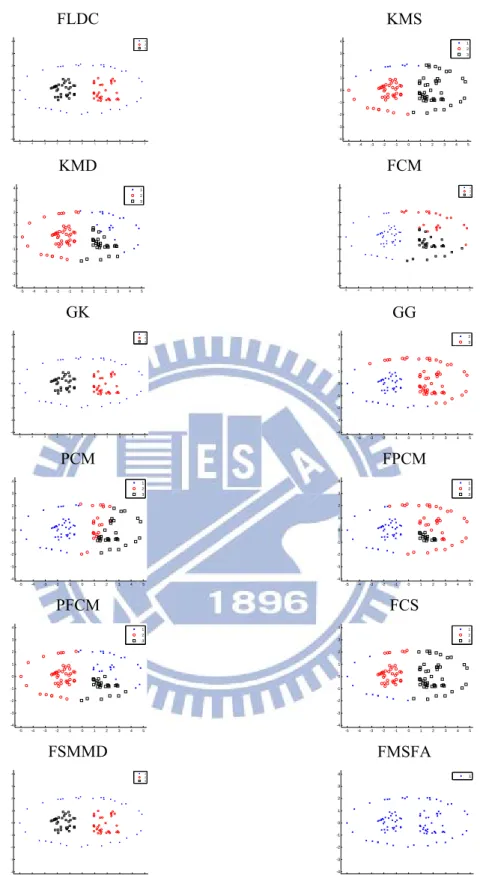
Figure 4. Ten artificial data sets [53]-[54] were used in this study. The first three data sets were generated with 10 additional noise features. The number of clusters appears in parentheses. ... 22
Figure 5. The results of clustering the “Four gauss” data set using twelve clustering algorithms. The best clustering results from applying GG and GGD were chosen for comparison. This figure also shows the best results of clustering FSMM and FSMMD for comparison. ... 26
Figure 6. The results of clustering the “Easy doughnut” data set using twelve clustering algorithms. The best clustering results from applying GG and GGD were chosen for comparison. This figure also shows the best results of clustering FSMM and FSMMD for comparison. ... 27
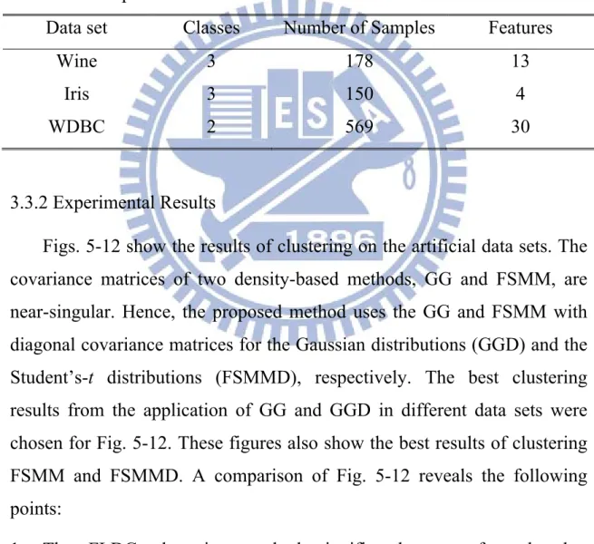
Figure 7. The results of clustering the “Difficult doughnut” data set using twelve clustering algorithms. The best clustering results from the application of GG and GGD were chosen for comparison. This figure also shows the best results of clustering FSMM and FSMMD for comparison. 28
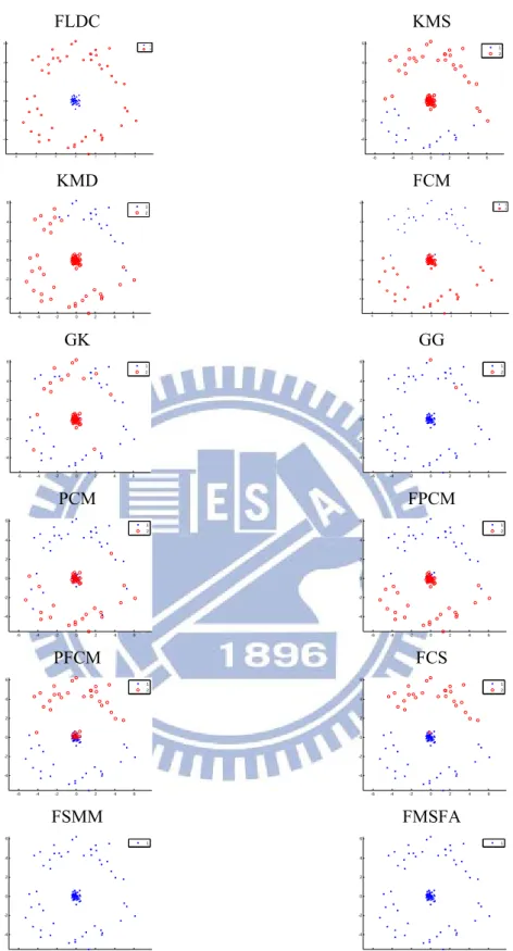
Figure 8. The results of clustering the “Boat” data set using twelve clustering algorithms. The best clustering results from applying GG and
GGD were chosen for comparison. This figure also shows the best results of clustering FSMM and FSMMD for comparison. ... 29
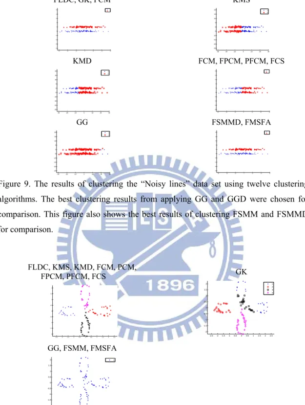
Figure 9. The results of clustering the “Noisy lines” data set using twelve clustering algorithms. The best clustering results from applying GG and GGD were chosen for comparison. This figure also shows the best results of clustering FSMM and FSMMD for comparison. ... 30
Figure 10. The results of clustering the “Petals” data set using twelve clustering algorithms. The best clustering results from applying GG and GGD were chosen for comparison. This figure also shows the best results of clustering FSMM and FSMMD for comparison. ... 30
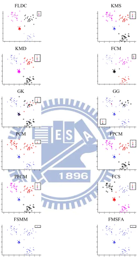
Figure 11. The results of clustering the “Saturn” data set using twelve clustering algorithms. The best clustering results from applying GG and GGD were chosen for comparison. This figure also shows the best results of clustering FSMM and FSMMD for comparison. ... 31
Figure 12. The results of clustering the “Regular” data set using twelve clustering algorithms. The best clustering results from applying GG and GGD were chosen for comparison. This figure also shows the best results of clustering FSMM and FSMMD for comparison. ... 32
Figure 13. Flowchart of the SVM+EM [31]. ... 37
Figure 14. Example of SVM+EM classification [31]. ... 39
Figure 15. The left and right images represent the first-order and second-order neighborhood systems in the original space, respectively. ... 41
Figure 16. Example of training and related context patterns in the feature space [32]. ... 41
Figure 17. The pixels enclosed by bold lines represent the first-order neighborhood system used in SCSVM. ... 43
Figure 18. An example of the spatial-contextual information with the second-order neighborhood system of pattern xi in the original space. ... 45
Figure 19. The left panel shows the decision boundary (solid black line) obtained by SVM. The center panel shows the semi-labels of the patterns in
the second-order neighborhood system of xj. The right panel shows the
decision boundary (solid red line) obtained of SCSVM. ... 46
Figure 20. A multiclass case of the spatial contextual information defined by the OAO strategy (class 1 versus class 2) for pattern xi in the neighborhood system O
i
x
. The labels of class 1 and class 2 are defined as +1 and -1, respectively. ... 47
Figure 21. A multiclass case of the spatial contextual information defined by the OAA strategy (class 1 versus all others) for pattern xi in the neighborhood system O
i
x
. The label of class 1 is defined as +1 and the labels of the remaining classes (class 2 and class 3) are defined as -1. ... 48
Figure 22. SCSVM and SCSVMF classification systems. ... 51
Figure 23. A portion of the Indian pine site image measuring 145145 pixels. ... 52
Figure 24. The ground truth of the Indian pine site data set. ... 52
Figure 25. The false-color IR image of a portion of Washington D.C. Mall image measuring 205 307 pixels. There are seven categories: grass, tree, roof, water, road, trail, and shadow. ... 54
Figure 26. The overall accuracies in percentages of the experimental classifiers, SCSVM and SCSVMF, for the IPS data set. ... 57
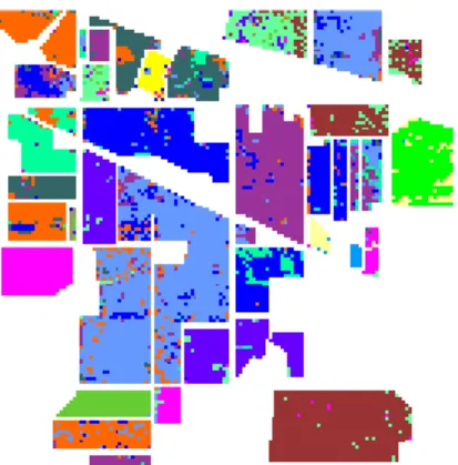
Figure 27. The classification maps of the IPS data set by the highest performance of each type classifier. ... 62
Figure 28. The overall accuracies in percentages of the experimental classifiers, SCSVM and SCSVMF, for the Washington D.C. Mall data set in case 1. ... 64
Figure 29. The overall accuracies in percentages of the experimental classifiers, SCSVM and SCSVMF, for the Washington D.C. Mall data set in case 2. ... 66
Figure 30. The overall accuracies in percentages of the experimental classifiers, SCSVM and SCSVMF, for the Washington D.C. Mall data set in case 3. ... 67
Figure 31. The classification maps of a portion of the Washington D.C. data set (case 3) by the highest performance of each type classifier. ... 73
Figure 32. The classification maps of a portion of the Washington D.C. data set (case 3) of SCSVM (OAO) and SCVM (OAA) with M=4 and different parameters =0, 0.1, and 0.3. ... 74
List of symbols
List of symbols
L : the number of clusters or classes N : the number of samples
n : the number of training samples
M : the number of samples in the neighborhood system
X : A hyperspectral d-dimensional image of size IJ pixels
D : the training data set
i
H : the set of samples in class i H :a Hilbert space
Ni : the number of samples in class i
R : the set of real numbers d
R : the d dimensional Euclidean space
R : the set of positive real numbers O
i x
: a neighborhood system w.r.t. xi in the original space
F i x
: a neighborhood system w.r.t. xi in the feature space x : an unlabeled pattern j x : the j-th sample ) ( x i
j : the j-th sample in class i ij
x : the j-th sample in the neighborhood system xi
i
c : the center of the cluster i or class i c : the total mean of samples
s
w : a normal vector to the decision hyperplane of support vector machine
ξ : the vector whose elements are slack variables of the support vector machine
ij
: the vector whose elements are slack variables of the context-sensitive semi-supervised support vector machine
ij
: the weights of the importances of context patterns in the context-sensitive semi-supervised support vector machine
α : the vector with elements that are Lagrange multipliers
d : the dimensionality of the original space m : the weighting exponent
p : the dimensionality of the reduced space
r : the regularization parameter of LDA-based clustering s
: the s-th large eigenvalue
ij
u : the membership grade of the j-th sample in cluster i
i
η : the tradeoff parameter of fuzzy compactness and separation
: the parameter to control ηi
i
y :the class label w.r.t. the training sample xi
ij
y :the semi-label of xij
b
:a constant to control the decision hyperplane of the support vector machinei
:a slack variable of the support vector machine w.r.t. xi
C : a penalty parameter of the support vector machine
i
: a Lagrange multiplier
: a nonnegative parameter that controls the effect of spatial-contextual information
FW
S : the fuzzy within-cluster scatter matrix
FB
S : the fuzzy between-cluster scatter matrix LDA
w
S : the with-class scatter matrix of linear discriminant analysis LDA
b
S : the between-class scatter matrix of linear discriminant analysis UFLDA
w
S : the with-class scatter matrix of LDA-based clustering ULDA
b
S : the between-class scatter matrix of LDA-based clustering
K : a kernel matrix
i
: a positive semi-definite matrix for computing an adaptive distance norm of Gustafson-Kessel algorithm
i
F : the fuzzy covariance matrix of Gustafson-Kessel algorithm
FCM
J : the cost function of fuzzy c-means
GK
J : the cost function of Gustafson-Kessel algorithm
FCS
J : the cost function of fuzzy compactness and separation
LDA
J : the objective function of linear discriminant analysis
FLDC
J : the objective function of LDA-based clustering
: a nonlinear feature mapping : a kernel function
SVM
f : the decision function of the support vector machine
SCSVM
f : the decision function of the spatial-contextual support vector machine
m : the function with the output being the number of pixels in the neighbor system belonging to class +1
m : the function with the output being the number of pixels in the neighbor system belonging to class -1
1. Introduction
Researchers have developed numerous statistical learning algorithms for applications in various areas of science, finance, and industry in recent years. Statistical learning comprises several different paradigms such as classification, regression, feature extraction, dimensionality reduction and density estimation [3]. The basic idea of classification methods for feature space data is to partition up the entire feature space into L exhaustive, nonoverlapping regions, where L is the number of classes present in the scene, so that every point in the feature space is uniquely associated with one of the L classes [22].
The classification algorithms can be divided into two main categories according to the learning process. Supervised classification, or simply classification, is the learning process of inferring a function to classify unknown patterns using the training data to train the rule [66], i.e., a set of training samples is available and the classifier exploits this a priori known information [2].
The other type of learning process is called unsupervised classification, or simply clustering. It is referred to as unsupervised because it does not use training samples [22]. Clustering assesses the relationships among samples of a data set by organizing the patterns into different groups. After clustering, patterns in one group show greater similarity to each other than those belonging to different groups without any prior known information [1]. Clustering analysis can detect underlying structures within data, for classification and pattern recognition, and for model reduction and optimization [2], [4]-[5].
Clustering algorithms are most commonly used as an aid to selecting a class list and training samples for the classes in that list. That is, clustering
may be a means of preprocessing the data for a supervised classification procedure. A clustering scheme may be applied to the data for each class separately and representative samples for each group within the class used as the prototypes for that class [66]. Fundamentally, to be optimally useful, a classification must have classes that are (simultaneously) “of information value, exhaustive, and separable.” The training samples for supervised learning generally are selected with emphasis on the former one. Clustering is a useful tool of the training process to achieve the latter two. It can be a useful procedure, though, in defining spectral classes and training for them by breaking up the distribution of pixels in feature space into subunits so that one can observe what is likely to be separable from what. It allows one to locate the prevailing modes in the feature space, if any prevalence exists [22].
Recent statistical learning algorithms [17]-[19] use both labeled and unlabeled samples for training. These algorithms are called semi-supervised learning process, and fall between unsupervised pattern recognition and supervised recognition. The aim of this thesis is to develop an unsupervised clustering algorithm and a semi-supervised classification algorithm. The former one is a fuzzy-based clustering which considers both within- and between-information of clusters, and the latter one is a semi-supervised classification algorithm which takes into account both spectral and spatial information.
Fuzzy-based clustering, which determines if a vector belongs to a specific cluster to a certain degree, have been the subject of intensive research in the past three decades [2], [4]-[8]. Fuzzy c-means (FCM) clustering is one of the most well-known clustering methods [7]-[8], and researchers have developed many advanced FCM-type clustering algorithms. The Gustafson-Kessel (GK) algorithm [9] is a well-known
algorithm in this category. This algorithm employs an adaptive distance norm to detect clusters of different geometrical shapes in one data set [2]. Krishnapuram and Keller [52] proposed a new clustering model, called possibilistic c-means (PCM), which relaxes the following constraint: “the sum of the membership values of every sample to all clusters is 1.” This approach avoids the outliers belonging to one or more clusters. In 1997, the fuzzy-possibilistic c-means (FPCM) [10] was proposed to generate both possibility and membership values. However, the possibility values generated by FPCM become very small as the size of the data set increases. To eliminate the problem of FPCM and take advantage of the benefits of FCM and PCM, the possibilistic fuzzy c-means (PFCM) was proposed in 2005 [11].
Some FCM-type algorithms, such as the Gath-Geva (GG) algorithm, employ an adaptive distance norm based on the fuzzy maximum likelihood estimates [5], [12]. Chatzis and Varvarigou [13] proposed a robust fuzzy clustering algorithm based on the fuzzy treatment of finite mixtures of multivariate Student’s t-distributions (FSMM). This approach uses finite mixtures of multivariate Student’s t distributions instead of finite Gaussian mixture models (GMMs). Chatzis and Varvarigou [56] combined the advantages of factor analysis and proposed a fuzzy mixture of Student’s t factor analyzers (FMSFA). FMSFA provides a well-established observation space dimensionality reduction framework for fuzzy clustering algorithms based on factor analysis. This simultaneously achieves fuzzy clustering and a reduction in local dimensionality within each cluster. Their experimental results show that FMSFA outperforms finite mixtures of Student’s t-factor analyzers (tMFA) [57], a modification of the fuzzy c-varieties algorithm with regularization by Kullback–Leibler information (KLFCV) [58], and the mixture of factor analyzers (MFA) model [59].
Most fuzzy-based clustering algorithm by minimizing a cost function, only based on the sum of distances between samples to their cluster centers [2], which is equal to the trace of the within-cluster scatter matrix [14]-[15]. Researchers have recently used linear discriminant analysis (LDA) [14] for dimensional reduction in supervised classification problems. LDA uses the mean vector and covariance matrix of each class to formulate within-class, between-class, and mixture-class scatter matrices. Two similar fuzzy-based clustering algorithms based on fuzzy within-cluster, between-cluster, and total scatter matrices are proposed in [15] and [16]. The objective function of fuzzy compactness and separation (FCS) [15] is based on the difference of fuzzy within- and between-cluster scatter matrices. This minimizes the measurement of compactness, but simultaneously maximizes the separation measure. However, the within- and between-class scatter matrices of LDA are not the special case of the proposed fuzzy within- and between-cluster scatter matrices in the supervised learning problem. Moreover, based on the Fisher criterion, the LDA method finds features such that the ratio of the between-class scatter to the average within-class scatter is maximized in a lower dimensional space. Of the concept of class scattering to class separation, the Fisher criterion takes the large values from samples when they are well clustered around their mean within each class, and the clusters of the different classes are well separated [2]. The Fisher criterion is formulated as a function of class statistics. For these reasons, this thesis proposes a clustering algorithm based the Fisher criterion [4].
The first part of the thesis is to propose a fuzzy-based clustering which is based on the fuzzy-based within- and between-cluster scatter matrices. In addition, the Fisher criterion is used to form the objective function. This means that the proposed clustering algorithm take into account not only the within- and between-information of the distribution of data but also the
interaction of the within- and between-information. Chapters 2-3 present the fuzzy-based clustering algorithm. Chapter 2 introduces some recently proposed fuzzy-based clustering algorithms. Chapter 3 details the proposed clustering algorithm based on both within- and between-cluster scatter matrices, extended from linear discriminant analysis (LDA) [4].
Figure 1. The spectral values obtained from the Indian Pine Site data set. The purple represents the Soybeans-min till patterns and the yellow represents the Corn-no till patterns. These two classes have similar spectral properties.
In hyperspectral image classification, spectral-domain based classifiers often lead to imprecise estimation of different land-cover classes that have very similar spectral properties, which makes it difficult to distinguish unlabeled patterns [20]-[21]. Fig. 1 shows the spectral values obtained from patterns of two categories in the Indian Pine Site data set: Soybeans-min till (purple color) and Corn-no till (yellow color) [22]. These two different classes have very similar spectral properties. Hence, employing these classes to train conventional classifiers (e.g., maximum likelihood classifier (ML) [2], [15], k-nearest neighbor classifier (k-NN) [2], [15], and support vector machine (SVM) [23]-[24]) leads to poor classification performance, producing a speckle-like classification map [20]-[21], [25]. Fig. 2 shows
that the support vector machine (SVM) classification map of Indian Pine Site includes a number of speckle-like errors.
Figure 2. The support vector machine (SVM) classification results of the Indian Pine Site image, containing speckle-like errors.
Considering both spectral and spatial-contextual information, using a semi-supervised learning algorithm is an effective way to decrease speckle-like errors when interpreting a hyperspectral image. There are two main methods for combining spectral and spatial-contextual information. The graph-based technique [18]-[19], [26]-[32] uses the typical method of performing a regularization in which “similar” features belong to the same class. This method associates the vertices of a graph with the complete set of samples, and then builds the regularization depending on the variables defined on the vertices [18]. The other approach is to use fixed-window-based methods, such as Markov random fields [20]-[21], morphological filtering [28], or morphological leveling [29]-[30]. This approach improves the classification performance of hyperspectral images compared to pixel-wise methods [31].
Jackson and Landgrebe [20] applied a Gaussian function to the Bayesian decision rule with Markov random fields (MRF), Bayesian contextual classifier based on MRF (ML_MRF), to mitigate the
speckle-like errors. Their method achieves improved performance in classification maps. Another study suggests applying similar concepts to develop a MRF-based k-nearest neighbors classifier and Parzen classifier [21]. However, MRF-based classifiers are still constrained by statistical estimation (e.g., the covariance matrix of ML based on a Gaussian distribution) or the amount of learning data.
The support vector machine [23] is a pattern classification technique proposed by Vapnik et al. Unlike traditional methods, which minimize empirical training errors, SVM attempts to minimize the upper bound of the generalization error by maximizing the margin between the separating hyperplane and the training data. Hence, SVM is a distribution-free algorithm that can overcome the problem of poor statistical estimation. SVM also achieves greater empirical accuracy and better generalization capabilities than other standard supervised classifiers [3] [34]-[35]. In particular, SVM performs well for high-dimensional data classification with a few training samples [37]-[38], and is robust to the Hughes phenomenon [32]-[33], [35], [37]-[38].
Moreover, many studies [30]-[33] show that support vector machines with both spectral and spatial information achieve effective and stable hyperspectral image classification. A context-sensitive semi-supervised support vector machine (CS4VM) [32] uses the context of neighborhood patterns as semi-patterns to solve the problem of noisy training patterns. In this case, noisy training patterns are mislabeled patterns that introduce distorted information to a classifier. CS4VM is a semi-learning approach in which the computational cost increases as the number of semi-samples increases.
Tarabalka et al. [31] presented a spectral-spatial classification scheme based on partitional clustering techniques (SVM+EM). This approach
segments an image into more homogeneous regions and combines the results of these regions using pixel-wise SVM classification. A spatial post-regularization (PR) of the classification map reduces the noise. This approach is particularly suitable for classifying images with large spatial structures, when spectral responses of different classes are dissimilar, and when classes contain a comparable number of pixels. If the spectral responses are not significantly different, this approach may result in misclassification [31].
The second part of this thesis uses two neighborhood systems, that one is in the original space and the other one is in the feature space, to modify the constrain and decision rule of the support vector machine, and proposes a spatial-contextual support vector machine to overcome the speckle-like errors. Chapters 4-5 focus on the spectral-spatial classification schemes. Chapter 4 introduces the SVM and some recently spectral-spatial classification algorithms. Chapter 5 describes two spatial-contextual support vector machine classification algorithms (SCSVMs) [39] that modifies the decision function and constraints of a support vector machine (SVM) using a spatial-contextual term in the original space or in the feature space, which are based on the concept of the Markov random fields in the original space or k-nearest neighborhoods in the feature space, respectively.
The thesis is devoted to fuzzy-based clustering algorithm, fuzzy linear discriminant clustering (FLDC), and semi-supervised image classification, spatial-contextual support vector machine. First, in Chapter 3, fuzzy-based within- and between-cluster scatter matrices extended from the within- and between-class scatter matrices of LDA are introduced. Furthermore, the Fisher criterion composed by the fuzzy-based scatter matrices is used to form the objective function. FLDC considers not only the within- and between-information of the data distribution but also the interaction of the
within- and between-information. The results of experiments on both synthetic and real data show that the proposed clustering algorithm can generate similar or better clustering results than eleven popular clustering algorithms: K-means, K-medoid, FCM, the Gustafson-Kessel, Gath-Geva, possibilistic c-means, fuzzy-possibilistic c-means, possibilistic fuzzy c-means, fuzzy compactness and separation, a fuzzy clustering algorithm based on a fuzzy treatment of finite mixtures of multivariate Student’s-t distributions algorithms, and a fuzzy mixture of Student’s t factor analyzers model.
Then, in Chapter 5, two neighborhood systems is used to overcome the similar spectrum problem in support vector machine. Two semi-supervised classifiers, spatial-contextual support vector machines (SCSVMs), are proposed by modifying the constrain and the decision function of support vector machine. To evaluate the effectiveness of SCSVM, the experiments in this study compare the performances of other classifiers: a support vector machine (SVM), context-sensitive semi-supervised support vector machine (CS4VM), maximum likelihood classifier (ML), Bayesian contextual classifier based on Markov random fields (ML_MRF), and k-nearest-neighbor classifier (k-NN). Experimental results show that the proposed method achieves good classification performance on famous hyperspectral images (the Indian Pine site and the Washington, D.C. Mall data sets). The overall classification accuracy of for the hyperspectral image of the Indian Pine site dataset with 16 classes is 95.5%. The kappa accuracy is up to 94.9%, and the average accuracy of each class is up to 94.2%.
2. Literature Review of Fuzzy-based Clustering
Algorithms
The aim of clustering algorithms is to identify unknown data structures, such as natural groups or clusters, by measuring the similarities between samples. The samples within a cluster or group are more similar to each other than those pixels belonging to other clusters [3], [40]. This section reviews some well-known fuzzy-based clustering algorithms.
2.1 Fuzzy C-means Clustering Algorithm
Fuzzy c-mean clustering (FCM) is the fuzzy equivalent of the nearest mean “hard” clustering algorithm [1]-[2], [5]-[6], [41], and minimizes the cost function
L i N j i j m ij i ij FCM u u J 1 1 2 c x ) ( ) c , (with respect to membership grade uij and ci, the center of fuzzy cluster i, where d
j R
x , N is the number of samples, L>1 is the number of clusters, and m(1,) is a weighting exponent.
The FCM algorithm assigns the memberships to xj . These memberships are inversely related to the relative distance of xj to the L cluster centers {ci}. The formulation of criterion JFCM could be regarded as the trace of the fuzzy within-cluster scatter matrix SFW [2], which is defined as
L i N j T i j i j m ij FW u S 1 1 ) c x )( c (x ) ( .Equation above is similar to the within-class scatter matrix of LDA in that this criterion only considers the within-cluster scatter matrix. A consideration the within-cluster similarity is the only criterion. Based on previous suggestions [34], the division into clusters should be characterized by within-cluster similarity and between-cluster (external) dissimilarity. This is the reason why this study applies the Fisher criterion.
2.2 Gustafson-Kessel algorithm
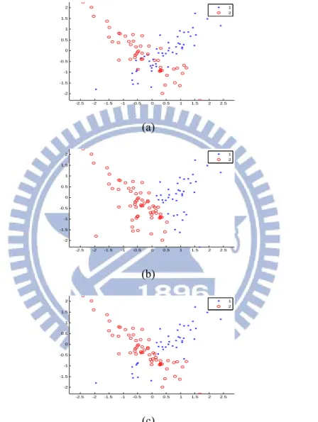
The Gustafson-Kessel (GK) algorithm [9] is a well-known example of FCM-type clustering algorithms. The GK algorithm employs an adaptive distance norm to detect clusters of different geometrical shapes in one data set [5]. FCM is suitable for clusters with similar distributions. If clusters with very different distributions like Fig. 3(a), the “x” remarks 50 random samples chosen from the multivariate normal distribution with mean
T ] 0 , 5 . 0 [ and covariance 8 . 0 7 . 0 7 . 0 8 . 0
, and the “o” remarks 50 random samples chosen from the multivariate normal distribution with mean
T ] 0 , 5 . 0 [ and covariance 8 . 0 7 . 0 7 . 0 8 . 0
, the clustering results of FCM (Fig. 3(b)) are frequently wrong, especially, on the left-bottom part of cluster 1 and the right-bottom part of cluster 2. The Gustafson-Kessel (GK) algorithm defines the fuzzy covariance matrices, which are used to compute generalized squared Mahalanobis distances, to solve this problem. Fig. 3(c) shows the clustering results of GK algorithm which is more similar to Fig. 3(a) than FCM. That is, the GK algorithm can detect clusters of different geometrical shapes in one data set.
The objective function of GK algorithm [9] is defined as
L i N j i j i T i j m ij i i ij GK u u J 1 1 ) c (x ) c (x ) ( ) , c , (where the matrices i , which adapt the distance norm to the local topological structure of the data [5], serve as optimization variables. Since
i
should be a positive definite matrix, the common approach is to constrain the determinant of i (i.e., det( )i i, i 0, i1,...,L).
-2.5 -2 -1.5 -1 -0.5 0 0.5 1 1.5 2 2.5 -2 -1.5 -1 -0.5 0 0.5 1 1.5 2 1 2 (a) -2.5 -2 -1.5 -1 -0.5 0 0.5 1 1.5 2 2.5 -2 -1.5 -1 -0.5 0 0.5 1 1.5 2 1 2 (b) -2.5 -2 -1.5 -1 -0.5 0 0.5 1 1.5 2 2.5 -2 -1.5 -1 -0.5 0 0.5 1 1.5 2 1 2 (c)
Figure 3. (a) The “x” remarks 50 random samples chosen from the multivariate normal
distribution with mean [0.5,0]T and covariance
8 . 0 7 . 0 7 . 0 8 . 0
, and the “o” remarks 50
random samples chosen from the multivariate normal distribution with mean [0.5,0]T
and covariance 8 . 0 7 . 0 7 . 0 8 . 0
; (b) The clustering results of (a) applying FCM; (c) the clustering results of (a) applying GK algorithm.
Using the Lagrange multiplier method, i is obtained by 1 / 1 )) det( ( d i i i i F F ,
where Fi is the fuzzy covariance matrix [5], [9] of the i-th cluster defined by:
N j m ij N j T i j i j m ij i u u F 1 1 ) ( ) c x )( c x ( ) ( .2.3 Fuzzy Compactness and Separation
Previous studies [15], [16] have proposed two similar fuzzy-based clustering algorithms based on fuzzy within-cluster, between-cluster, and total scatter matrices. The objective function of the fuzzy compactness and separation (FCS) [15] is based on fuzzy between- and within-cluster scatter matrices. This approach minimizes the measurement of compactness, and simultaneously maximizes the separation measure.
The fuzzy between-cluster scatter matrix SFB and within-cluster scatter matrix SFW are defined as
c i n j T j j m ij i FB u S 1 1 ) c x )( c x ( ) ( and
c i n j T i j i j m ij FW u S 1 1 ) c x )( c x ( ) ( where
N i j N 1 x 1c . The objective function of FCS is defined as
. c x ) ( c x ) ( ) ( tr ) ( tr ) c , ( 1 1 2 1 1 2
L i N j j m ij i L i N j i j m ij FB FW i ij FCS u u S S u J By minimizingJFCS, the proposed method uses the following equations to mutually update each other:
L k m k k k j m i i i j ij u 1 ) 1 /( 1 2 2 ) 1 /( 1 2 2 ) || c c || || c x (|| ) || c c || || c x (|| and
n j m ij i N j m ij n j m ij i N j j m ij i u u u 1 1 1 1 ) ( ) ( c ) u ( x ) ( c ,where the parameter could be set up with i
, || c c || max || c c || min ) 4 / ( 2 2 k k i i i i i
and [0,1] is the parameter to be pre-determined. The objective function proposed by Yin et al. [43] is a special case of FCS in which the parameters are all set to i 1/(L(L1)).
The Fisher criterion, the trace of the product of the inverse of the within-class scatter matrix and the between-class scatter matrix, takes large values when samples are well clustered, around their mean within each class, and the clusters of the different classes are well separated [2].This approach is widely used in different applications [42], [43]-[44]. The following discussion introduces new definitions of unsupervised cluster scatter matrices. The corresponding objective function is based on the Fisher criterion including the interaction of cluster scatter matrices.
2.4 Other FCM-type Clustering Algorithms
Krishnapuram and Keller [52] proposed a new clustering model, called possibilistic c-means (PCM), that relaxes a constraint (“the sum of the membership values of every sample to all clusters is 1”) to interpret the membership function or degree of typicality in a possibilistic sense [45]. The fuzzy-possibilistic c-means (FPCM) [10] was proposed in 1997 to generate both possibility and membership values. However, the possibility values generated by FPCM become very small as the size of the data set increases. To eliminate the problem of FPCM and take advantage of the benefits of FCM and PCM, the possibilistic fuzzy c-means (PFCM) was proposed in 2005 [46].
Some FCM-type algorithms, such as the Gath-Geva (GG) algorithm, employ an adaptive distance norm based on the fuzzy maximum likelihood estimates [2], [30]. Chatzis and Varvarigou [27] proposed a robust fuzzy clustering algorithm based on a fuzzy treatment of finite mixtures of multivariate Student’s-t distributions (FSMM). This approach uses finite mixtures of multivariate Student’s t distributions instead of finite Gaussian mixture models (GMMs).
3. LDA-based Clustering Algorithm
This chapter introduces a novel clustering algorithm, called fuzzy linear discriminant clustering (FLDC), that accounts both within- and between-cluster information [4]. Since the scatter matrices are extended from the LDA, Section 3.1 reviews the LDA.
3.1 Review of LDA
LDA is often used for dimension reduction in classification problems. Because it uses the mean vector and covariance matrix of each class, LDA is often referred to as the parametric feature extraction method [14]. Within-class, between class, and mixture scatter matrices are frequently used to formulate the criterion of class separability.
Suppose that i d N i i R H i {x(),...,x()}
1 are the set of samples in class i,
i
N is the number of samples in class i, i1,...,L, and N N1NL is the number of all training samples. LDA defines the between-class scatter matrix LDA
b
S and the within-class scatter matrix LDA w S as
L i T i i i LDA b N N S 1 ) c c )( c c ( and
L i N j T i i j i i j LDA w i N S 1 1 ) ( ) ( c )(x c ) x ( 1where ci is the class mean defined by
i N j i j i i N 1 ) ( x 1 c and
L i N j i j i N 1 1 ) ( x 1The optimal features are determined by optimizing the Fisher criterion 1 J JLDA given by ] ) [( tr 1 LDA b LDA w LDA S S J .
This is equivalent to solving the generalized eigenvalue problem,
s LDA w s s LDA b S S v v , s 1 , ,d with 1 2 d ,
where the extracted eigenvectors form the transformation matrix of LDA. In other words, the transformation matrix from the original space to the reduced subspace is defined by
] v , , v , [v1 2 p A .
The Fisher criterion JLDA can detect the separability of the transformed training samples, but LDA is a supervised feature extraction. The following section proposes the between- and within-cluster scatter matrices of an unsupervised LDA based on the concept of membership values and cluster means of FCM as a clustering algorithm and an unsupervised feature extraction.
3.2 FLDC Algorithm
The proposed method derives two fuzzy between and within-cluster scatter matrices from the scatter matrices of LDA, and uses them to
formulate FLDC. The fuzzy between-cluster scatter matrix FLDA b
S and the fuzzy within-cluster scatter matrix FLDA
w S are defined as
L i T i i N j ij FLDA b N u S 1 1 ) c c )( c c ( and
c i N j T i j i j ij FLDA w N u S 1 1 ) c x )( c x ( , where
N j j N k ik ij i u u 1 1 x cis the class mean, which is the same as FCM, and
N i j N c 1 x 1 represents the total mean. The following theorem shows that the between- and within-class scatter matrices of LDA are special cases of the proposed
FLDA b
S and FLDA w
S , respectively.
Theorem 1: In the supervised situation, if
i j i j ij H if H if u x 0 x 1
for all 1i L and 1 j N ,
then, the proposed FLDA b
S and FLDA w
S are the same as LDA b S and LDA w S , respectively. Proof:
Suppose there are Ni samples in Hi for i1 , ,L , and
i N
k uik N
i i j N j i j i H j i N j j N k ik ij i N N u u 1 ) ( x 1 1 x 1 x 1 x cis the same as the class mean in LDA and the fuzzy between-cluster scatter matrix . ) c c )( c c ( ) c c )( c c ( 1 1 1 LDA b L i T i i i L i T i i N j ij FLDA b S N N N u S
The fuzzy within-cluster scatter matrix is then
. ) c x )( c x ( 1 ) c x )( c x ( ) c x )( c x ( 1 ) ( ) ( 1 1 1 1 LDA w c i T i i j i i j N j c i x H T i j i j ij c i N j T i j i j ij FLDA w S N N u N u S i i j
□ Based on this theorem and the objective function of LDA, the general objective function of FLDC is defined by] ) [( tr ) ( 1 FLDA b FLDA w ij FLDC u S S J ,
including the interaction of FLDA b
S and FLDA w
S . This study considers the interaction of the fuzzy between- and within-cluster scatter matrices in the Fisher criterion. Results for artificial data sets show that FLDC can detect the clusters with the largest between-cluster separability.
To reduce the effects of the cross products of within-class distances and prevent singularity, some regularized techniques [47]-[48] can be applied to the fuzzy within-cluster scatter matrix. In FLDC, the fuzzy within-cluster scatter matrix is regularized by
) ( diag ) 1 ( FLDA w FLDA w FLDA rw rS r S S
where diag( FLDA) w
S is the diagonal parts of matrix FLDA w
S and r[0,1] is a regularization parameter.
The proposed clustering algorithm defines the optimization problem as follows: ] ) [( max arg ) ( max arg 1 FLDA b FLDA rw U ij FLDC U FLDC J u S S U which constrains L u j N i ij 1, 1, , 1
. Because the optimization problem is nonlinear and non-convex, several popular optimization algorithms [49]-[50] can be applied to solve this problem: “interior-point,” “active-set,” and “trust-region-reflective.” In implementing these algorithms, the “active-set” algorithm has a lower cost time than the other two algorithms, but it is sensitive to the initial value. Hence, the “interior-point” algorithm is used to find the optimizer UFLDC in this study. However, the “interior-point” algorithm has the highest corresponding time cost.
The decision rule, i.e., the defuzzification process, for the sample j is
kj k u
i argmax .
3.3 Experiments
3.3.1 Experimental Data and Designs
The experiments in this study validate the performance of the proposed FLDC using ten artificial data sets and three real data sets. This section compares the results of several algorithms on artificial and real data sets. These algorithms include the clustering FLDC, K-means (KMS), and K-medoid (KMD), FCM, Gustafson-Kessel (GK), Gath-Geva (GG) [5], possibilistic c-means (PCM) [52], fuzzy-possibilistic c-means (FPCM) [10],
possibilistic fuzzy c-means (PFCM) [11], fuzzy compactness and separation (FCS) [15], FSMM [13], and FMSFA [56] algorithms. The parameters r in FLDC and in FCS were set to 0.5. The weighting exponents of FCM, GK, GG, and PCM were set to m{2,4}. The weighting exponents of FPCM and PFCM were set to m{2,4} and
} 4 , 2 {
. The FSMM parameters were set to the default values in [51]. The FMSFA clustering results were the best results within the given set
} 5 . 1 , 1 , 5 . 0
{ of the model’s degrees of fuzziness of the fuzzy membership values.
To avoid the influence of initialization, all clustering algorithms were evaluated based on 3 real data sets and 100 randomly generated initial values for each data set. This study calculates and compares the mean, standard deviation, maximum, and minimum accuracy of the 100 clustering accuracy. The accuracy of the clustering is the proportion of correctly clustered data in the data set (i.e., clustering accuracy=(the number of correctly clustered data)/(the number of all samples)).
Fig. 4 shows 10 artificial data sets [53]:“Four-gauss data” (4 clusters), “Easy doughnut data” (2 clusters), “Difficult doughnut data” (2 clusters), “Boat data” (3 clusters), “Noisy lines data” (2 cluster), “Petals data”, (4 clusters), “Saturn data” (2 clusters), “Regular data” (16 clusters), “Half-ring data” (2 cluster), and “Spirals data” (2 clusters). These data sets can be downloaded from [54]. All data sets were created in two dimensions to present challenges in varying degrees. Ten dimensions of uniformly random noise were appended to each of the first three data sets (four gauss, easy doughnut, and difficult doughnut), while the other seven data sets were kept as two-dimensional. The last two data sets were omitted because the clustering results obtained of all clustering algorithms are similar.
Four gauss (4) Easy doughnut (2)
Difficult doughnut (2) Boat (3)
Noisy lines (2)
Petals (4)
Saturn (2) Regular (16)
Half rings (2) Two spirals (2)
Figure 4. Ten artificial data sets [53]-[54] were used in this study. The first three data sets were generated with 10 additional noise features. The number of clusters appears in parentheses.
Table 1 presents the real data sets used in this study: “Wine,” “Iris,” and “Breast Cancer Wisconsin (Diagnostic)” (WDBC). The Wine data set is a collection of data from three classes of wine from various locations in Italy. The Iris data set contains three classes of Iris flowers collected from Hawaii: Iris Setosa, Iris Versicolour, and Iris Virginica. There are two classes, benign and malignant, in the WDBC data set. These data sets are available from the FTP server of the UCI [55] data repository.
Table 1 Descriptions of Three Real Data Sets
Data set Classes Number of Samples Features
Wine 3 178 13
Iris 3 150 4
WDBC 2 569 30
3.3.2 Experimental Results
Figs. 5-12 show the results of clustering on the artificial data sets. The covariance matrices of two density-based methods, GG and FSMM, are near-singular. Hence, the proposed method uses the GG and FSMM with diagonal covariance matrices for the Gaussian distributions (GGD) and the Student’s-t distributions (FSMMD), respectively. The best clustering results from the application of GG and GGD in different data sets were chosen for Fig. 5-12. These figures also show the best results of clustering FSMM and FSMMD. A comparison of Fig. 5-12 reveals the following points:
1. The FLDC clustering method significantly outperformed other methods for the normal-like distribution of data (e.g., the four-gauss, easy doughnut, difficult doughnut, boat, and petals data sets) because it
considers the interaction of the between- and within-cluster scatter matrices. For the easy doughnut and difficult doughnut data sets, all algorithms had poor clustering results except FLDC.
2. The FLDC achieved the best performance with regular and noisy lines data sets.
3. KMS, KMD, FCM, FPCM, PFCM, and FCS only performed well on the four gauss and petals data sets.
4. PCM performs well only on the petals and noisy lines data sets.
5. GK employed an adaptive norm that estimates covariance matrices for each cluster. Hence, the GK algorithm can detect clusters with different geometrical shapes. and performed well on the boat and noisy lines data sets. However, its performance was dismal for the four gauss, easy doughnut, and difficult doughnut data sets.
6. Although FLDC performed poorly on the Saturn, half rings, and two spirals data sets, it was able to detect the clusters with the largest between-cluster separability in the Saturn data set. FLDC was unsuitable for the Saturn, half rings, and two spirals data, as these were complex nonlinear problems. The kernel method may be a way to solve these types of data sets.
7. The distribution-based clustering algorithms, including GG, FSMM, and FMSFA, performed poorly on the four gauss, easy doughnut, petals, and regular data sets because the covariance matrices of the density-based methods are near-singular.
8. FSMMD was able to improve the performance of FSMM on the boat and noisy lines data sets.
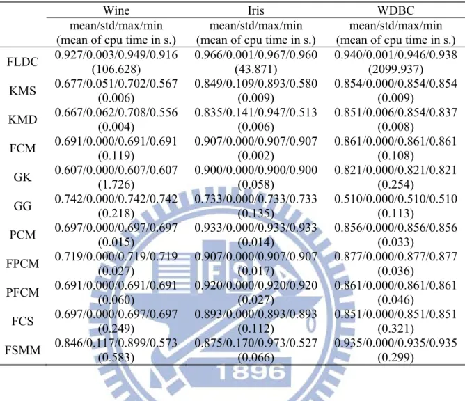
Table 2 shows the clustering accuracy in real data sets. The highest mean clustering accuracy for each data set (in rows) is shaded. Table 2
shows that the highest mean accuracies among all methods were 0.927, 0.966, and 0.940. All of these results were obtained by performing FLDC. Table 3 shows the accuracy of the three real data sets after applying FMSFA. The maximum accuracies of these data sets were 1, 0.980, and 0.949, respectively. However, it is very sensitive to the initial value. Hence, the highest average accuracies in every column were only 0.945, 0.774, and 0.882. The FSMM is more stable than FMSFA because it uses the results of clustering KMS as the initial value.
FLDC -6 -4 -2 0 2 4 6 8 -4 -2 0 2 4 6 1 2 3 4 KMS -6 -4 -2 0 2 4 6 8 -4 -2 0 2 4 6 1 2 3 4 KMD -6 -4 -2 0 2 4 6 8 -4 -2 0 2 4 6 1 2 3 4 FCM -6 -4 -2 0 2 4 6 8 -4 -2 0 2 4 6 1 2 3 4 GK -6 -4 -2 0 2 4 6 8 -4 -2 0 2 4 6 2 3 4 GG -6 -4 -2 0 2 4 6 8 -4 -2 0 2 4 6 1 2 3 PCM -6 -4 -2 0 2 4 6 8 -4 -2 0 2 4 6 2 4 FPCM -6 -4 -2 0 2 4 6 8 -4 -2 0 2 4 6 1 2 3 4 PFCM -6 -4 -2 0 2 4 6 8 -4 -2 0 2 4 6 1 2 3 4 FCS -6 -4 -2 0 2 4 6 8 -4 -2 0 2 4 6 1 2 3 4 FSMM -6 -4 -2 0 2 4 6 8 -4 -2 0 2 4 6 1 FMSFA -6 -4 -2 0 2 4 6 8 -4 -2 0 2 4 6 1
Figure 5. The results of clustering the “Four gauss” data set using twelve clustering algorithms. The best clustering results from applying GG and GGD were chosen for comparison. This figure also shows the best results of clustering FSMM and FSMMD for comparison.
FLDC -6 -4 -2 0 2 4 6 -4 -2 0 2 4 6 1 2 KMS -6 -4 -2 0 2 4 6 -4 -2 0 2 4 6 1 2 KMD -6 -4 -2 0 2 4 6 -4 -2 0 2 4 6 1 2 FCM -6 -4 -2 0 2 4 6 -4 -2 0 2 4 6 1 2 GK -6 -4 -2 0 2 4 6 -4 -2 0 2 4 6 1 2 GG -6 -4 -2 0 2 4 6 -4 -2 0 2 4 6 1 2 PCM -6 -4 -2 0 2 4 6 -4 -2 0 2 4 6 1 2 FPCM -6 -4 -2 0 2 4 6 -4 -2 0 2 4 6 1 2 PFCM -6 -4 -2 0 2 4 6 -4 -2 0 2 4 6 1 2 FCS -6 -4 -2 0 2 4 6 -4 -2 0 2 4 6 1 2 FSMM -6 -4 -2 0 2 4 6 -4 -2 0 2 4 6 1 FMSFA -6 -4 -2 0 2 4 6 -4 -2 0 2 4 6 1
Figure 6. The results of clustering the “Easy doughnut” data set using twelve clustering algorithms. The best clustering results from applying GG and GGD were chosen for comparison. This figure also shows the best results of clustering FSMM and FSMMD for comparison.
FLDC -8 -6 -4 -2 0 2 4 6 -6 -4 -2 0 2 4 6 1 2 KMS -8 -6 -4 -2 0 2 4 6 -6 -4 -2 0 2 4 6 1 2 KMD -8 -6 -4 -2 0 2 4 6 -6 -4 -2 0 2 4 6 1 2 FCM -8 -6 -4 -2 0 2 4 6 -6 -4 -2 0 2 4 6 1 2 GK -8 -6 -4 -2 0 2 4 6 -6 -4 -2 0 2 4 6 1 2 GG -8 -6 -4 -2 0 2 4 6 -6 -4 -2 0 2 4 6 1 2 PCM -8 -6 -4 -2 0 2 4 6 -6 -4 -2 0 2 4 6 1 2 FPCM -8 -6 -4 -2 0 2 4 6 -6 -4 -2 0 2 4 6 1 2 PFCM -8 -6 -4 -2 0 2 4 6 -6 -4 -2 0 2 4 6 1 2 FCS -8 -6 -4 -2 0 2 4 6 -6 -4 -2 0 2 4 6 1 2 FSMM -8 -6 -4 -2 0 2 4 6 -6 -4 -2 0 2 4 6 1 FMSFA -8 -6 -4 -2 0 2 4 6 -6 -4 -2 0 2 4 6 1
Figure 7. The results of clustering the “Difficult doughnut” data set using twelve clustering algorithms. The best clustering results from the application of GG and GGD were chosen for comparison. This figure also shows the best results of clustering FSMM and FSMMD for comparison.
FLDC -5 -4 -3 -2 -1 0 1 2 3 4 5 -4 -3 -2 -1 0 1 2 3 4 1 2 3 KMS -5 -4 -3 -2 -1 0 1 2 3 4 5 -4 -3 -2 -1 0 1 2 3 4 1 2 3 KMD -5 -4 -3 -2 -1 0 1 2 3 4 5 -4 -3 -2 -1 0 1 2 3 4 1 2 3 FCM -5 -4 -3 -2 -1 0 1 2 3 4 5 -4 -3 -2 -1 0 1 2 3 4 1 2 3 GK -5 -4 -3 -2 -1 0 1 2 3 4 5 -4 -3 -2 -1 0 1 2 3 4 1 2 3 GG -5 -4 -3 -2 -1 0 1 2 3 4 5 -4 -3 -2 -1 0 1 2 3 4 2 3 PCM -5 -4 -3 -2 -1 0 1 2 3 4 5 -4 -3 -2 -1 0 1 2 3 4 1 2 3 FPCM -5 -4 -3 -2 -1 0 1 2 3 4 5 -4 -3 -2 -1 0 1 2 3 4 1 2 3 PFCM -5 -4 -3 -2 -1 0 1 2 3 4 5 -4 -3 -2 -1 0 1 2 3 4 1 2 3 FCS -5 -4 -3 -2 -1 0 1 2 3 4 5 -4 -3 -2 -1 0 1 2 3 4 1 2 3 FSMMD -5 -4 -3 -2 -1 0 1 2 3 4 5 -4 -3 -2 -1 0 1 2 3 4 1 2 3 FMSFA -5 -4 -3 -2 -1 0 1 2 3 4 5 -4 -3 -2 -1 0 1 2 3 4 1
Figure 8. The results of clustering the “Boat” data set using twelve clustering algorithms. The best clustering results from applying GG and GGD were chosen for comparison. This figure also shows the best results of clustering FSMM and FSMMD for comparison.
FLDC, GK, PCM -30 -20 -10 0 10 20 30 -25 -20 -15 -10 -5 0 5 10 15 20 1 2 KMS -30 -20 -10 0 10 20 30 -25 -20 -15 -10 -5 0 5 10 15 20 1 2 KMD -30 -20 -10 0 10 20 30 -25 -20 -15 -10 -5 0 5 10 15 20 1 2 FCM, FPCM, PFCM, FCS -30 -20 -10 0 10 20 30 -25 -20 -15 -10 -5 0 5 10 15 20 1 2 GG -30 -20 -10 0 10 20 30 -25 -20 -15 -10 -5 0 5 10 15 20 1 2 FSMMD, FMSFA -30 -20 -10 0 10 20 30 -25 -20 -15 -10 -5 0 5 10 15 20 1 2
Figure 9. The results of clustering the “Noisy lines” data set using twelve clustering algorithms. The best clustering results from applying GG and GGD were chosen for comparison. This figure also shows the best results of clustering FSMM and FSMMD for comparison. FLDC, KMS, KMD, FCM, PCM, FPCM, PFCM, FCS -2.5 -2 -1.5 -1 -0.5 0 0.5 1 1.5 2 2.5 -2 -1.5 -1 -0.5 0 0.5 1 1.5 2 GK -2.5 -2 -1.5 -1 -0.5 0 0.5 1 1.5 2 2.5 -2 -1.5 -1 -0.5 0 0.5 1 1.5 2 1 2 3 4 GG, FSMM, FMSFA -2.5 -2 -1.5 -1 -0.5 0 0.5 1 1.5 2 2.5 -2 -1.5 -1 -0.5 0 0.5 1 1.5 2 4
Figure 10. The results of clustering the “Petals” data set using twelve clustering algorithms. The best clustering results from applying GG and GGD were chosen for comparison. This figure also shows the best results of clustering FSMM and FSMMD for comparison.
FLDC -5 -4 -3 -2 -1 0 1 2 3 4 5 -4 -3 -2 -1 0 1 2 3 4 1 2 KMS -5 -4 -3 -2 -1 0 1 2 3 4 5 -4 -3 -2 -1 0 1 2 3 4 1 2 KMD -5 -4 -3 -2 -1 0 1 2 3 4 5 -4 -3 -2 -1 0 1 2 3 4 1 2 FCM -5 -4 -3 -2 -1 0 1 2 3 4 5 -4 -3 -2 -1 0 1 2 3 4 1 2 GK -5 -4 -3 -2 -1 0 1 2 3 4 5 -4 -3 -2 -1 0 1 2 3 4 1 2 GG -5 -4 -3 -2 -1 0 1 2 3 4 5 -4 -3 -2 -1 0 1 2 3 4 1 2 PCM -5 -4 -3 -2 -1 0 1 2 3 4 5 -4 -3 -2 -1 0 1 2 3 4 1 2 FPCM -5 -4 -3 -2 -1 0 1 2 3 4 5 -4 -3 -2 -1 0 1 2 3 4 1 2 PFCM -5 -4 -3 -2 -1 0 1 2 3 4 5 -4 -3 -2 -1 0 1 2 3 4 1 2 FCS -5 -4 -3 -2 -1 0 1 2 3 4 5 -4 -3 -2 -1 0 1 2 3 4 1 2 FSMMD -5 -4 -3 -2 -1 0 1 2 3 4 5 -4 -3 -2 -1 0 1 2 3 4 1 2 FMSFA -5 -4 -3 -2 -1 0 1 2 3 4 5 -4 -3 -2 -1 0 1 2 3 4 1 2
Figure 11. The results of clustering the “Saturn” data set using twelve clustering algorithms. The best clustering results from applying GG and GGD were chosen for comparison. This figure also shows the best results of clustering FSMM and FSMMD for comparison.
FLDC 2 4 6 8 10 12 14 16 18 20 22 2 4 6 8 10 12 14 16 18 20 22 1 2 3 4 5 6 7 8 9 10 11 12 13 14 15 16 KMS 0 5 10 15 20 2 4 6 8 10 12 14 16 18 20 22 1 2 3 4 5 6 7 8 9 10 11 12 13 14 15 16 KMD 0 5 10 15 20 2 4 6 8 10 12 14 16 18 20 22 1 2 3 4 5 6 7 8 9 10 11 12 13 14 15 16 FCM 0 5 10 15 20 2 4 6 8 10 12 14 16 18 20 22 1 2 3 4 5 6 7 8 9 10 11 12 13 14 15 16 GK 0 5 10 15 20 2 4 6 8 10 12 14 16 18 20 22 1 2 3 4 5 6 7 8 9 10 11 12 13 14 15 16 GGD 0 5 10 15 20 2 4 6 8 10 12 14 16 18 20 22 14 16 PCM 0 5 10 15 20 2 4 6 8 10 12 14 16 18 20 22 1 2 3 4 5 6 7 8 9 10 11 12 13 14 15 16 FPCM 0 5 10 15 20 2 4 6 8 10 12 14 16 18 20 22 1 2 3 4 5 6 7 8 9 10 11 12 13 14 15 16 PFCM 0 5 10 15 20 2 4 6 8 10 12 14 16 18 20 22 1 2 3 4 5 6 7 8 9 10 11 12 13 14 15 16 FCS 0 5 10 15 20 2 4 6 8 10 12 14 16 18 20 22 1 2 3 4 5 6 7 8 9 10 11 12 13 14 15 16 FSMM 0 5 10 15 20 2 4 6 8 10 12 14 16 18 20 22 1 FMSFA 0 5 10 15 20 2 4 6 8 10 12 14 16 18 20 22 1
Figure 12. The results of clustering the “Regular” data set using twelve clustering algorithms. The best clustering results from applying GG and GGD were chosen for comparison. This figure also shows the best results of clustering FSMM and FSMMD for comparison.
Table 2 The Mean, Standard Deviation, Maximum, and Minimum Accuracy of Clustering for Three Real Data sets.
Wine Iris WDBC mean/std/max/min
(mean of cpu time in s.) (mean of cpu time in s.) mean/std/max/min (mean of cpu time in s.) mean/std/max/min
FLDC 0.927/0.003/0.949/0.916(106.628) 0.966/0.001/0.967/0.960(43.871) 0.940/0.001/0.946/0.938(2099.937) KMS 0.677/0.051/0.702/0.567(0.006) 0.849/0.109/0.893/0.580(0.009) 0.854/0.000/0.854/0.854(0.009) KMD 0.667/0.062/0.708/0.556(0.004) 0.835/0.141/0.947/0.513(0.006) 0.851/0.006/0.854/0.837(0.008) FCM 0.691/0.000/0.691/0.691 (0.119) 0.907/0.000/0.907/0.907 (0.002) 0.861/0.000/0.861/0.861 (0.108) GK 0.607/0.000/0.607/0.607(1.726) 0.900/0.000/0.900/0.900(0.058) 0.821/0.000/0.821/0.821(0.254) GG 0.742/0.000/0.742/0.742(0.218) 0.733/0.000/0.733/0.733(0.135) 0.510/0.000/0.510/0.510(0.113) PCM 0.697/0.000/0.697/0.697(0.015) 0.933/0.000/0.933/0.933(0.014) 0.856/0.000/0.856/0.856(0.033) FPCM 0.719/0.000/0.719/0.719(0.027) 0.907/0.000/0.907/0.907(0.017) 0.877/0.000/0.877/0.877(0.036) PFCM 0.691/0.000/0.691/0.691 (0.060) 0.920/0.000/0.920/0.920 (0.027) 0.861/0.000/0.861/0.861 (0.046) FCS 0.697/0.000/0.697/0.697(0.249) 0.893/0.000/0.893/0.893(0.112) 0.851/0.000/0.851/0.851(0.321) FSMM 0.846/0.117/0.899/0.573(0.583) 0.875/0.170/0.973/0.527(0.066) 0.935/0.000/0.935/0.935(0.299)
Table 3 The Mean, Standard Deviation, Maximum, and Minimum Accuracy of Clustering for Three Real Data sets of FMSFA, Where LD Represents the Latent Dimension
Wine Iris WDBC mean/std/max/min mean/std/max/min mean/std/max/min
FMSFA LD=1 0.898/0.085/0.955/0.854 0.774/0.154/0.980/0.333 0.813/0.005/0.821/0.803 FMSFA LD=2 0.945/0.069/0.966/0.579 0.768/0.127/0.967/0.333 0.882/0.000/0.882/0.882 FMSFA LD=3 0.891/0.143/1.000/0.539 0.704/0.105/0.967/0.333 0.865/0.027/0.949/0.715

![Figure 4. Ten artificial data sets [53]-[54] were used in this study. The first three data sets were generated with 10 additional noise features](https://thumb-ap.123doks.com/thumbv2/9libinfo/8391614.178725/38.892.253.753.120.918/figure-artificial-data-study-generated-additional-noise-features.webp)