基於行動定位服務的即時旅行時間知識庫預測系統

國

立

交

通

大

學

資訊科學與工程研究所

碩

士

論

文

基

於

行

動

定

位

服

務

的

即 時 旅 行 時 間 知 識 庫 預 測 系 統

A Knowledge Based Real-Time Travel Time Prediction

System using Location Based Service

研 究 生：蔡昇翰

指導教授：曾憲雄 教授

基於行動定位服務的即時旅行時間知識庫預測系統

A Knowledge Based Real-Time Travel Time Prediction System using

Location Based Service

研 究 生：蔡昇翰 Student：Sheng-Han Tsai

指導教授：曾憲雄 博士 Advisor：Dr. Shian-Shyong Tseng

國 立 交 通 大 學

資 訊 科 學 與 工 程 研 究 所

碩 士 論 文

A Thesis

Submitted to Institute of Computer Science and Engineering College of Computer Science

National Chiao Tung University in partial Fulfillment of the Requirements

for the Degree of Master

in

Computer Science June 2006

Hsinchu, Taiwan, Republic of China

基於行動定位服務的即時旅行時間

知識庫預測系統

研究生：蔡昇翰 指導教授：曾憲雄 博士 國立交通大學資訊學院 資訊科學與工程研究所

摘要

發展智慧型運輸系統(ITS) 的精神和目的就是利用先進的通訊技術、交通控制 與資訊來達到便利、經濟以及安全的交通環境。在 ITS 領域中，即時旅行時間預 測一直是被探討的重要題目。因為在 ITS 九大領域之中，即時旅行時間預測涵蓋 了其中的四個子領域：先進交通管理系統(ATMS)、先進旅行者資訊系統(ATIS)、 商用車輛營運系統(CVO)與急難救助系統(EMS)。並且它代表著交通路況的有用資 訊指標。 然而，在很多過去文獻中，旅行時間都被預測在高速公路和少數幹道路網上。 因為即時旅行時間是較難以預測在都會路網上，其中有四種原因是: 都會路網的複 雜度和繞路的問題，即時交通資訊如何取得的成本問題，有限的交通時間和空間 資訊收集問題，以及缺乏交通事件反應問題。本論文提出一個即時旅行時間知識 庫預測系統，其利用資料探勘技術與行動定位服務來找出一些過去的交通樣本， 並利用這些樣本和即時交通資訊來預測即時旅行時間。當交通事件發生在一些路 段上時，系統會觸發元規則(Meta-rule)來動態整合過去和現在的旅行時間預測。此 系統被實作在台北都會路網上，且實驗數據顯示動態整合歷史和即時的旅行時間 預測會比單一預測在過去或即時路況上得到較佳的結果。 關鍵字：旅行時間預測、資料探勘、專家系統、區域定位服務、智慧型運輸系統。

A Knowledge Based Real-Time Travel Time Prediction

System using Location Based Service

Student: Sheng-Han Tsai Advisor: Dr. Shian-Shyong Tseng Institute of Computer Science Engineering

National Chiao Tung University

Abstract

The purpose and the essence of developing Intelligent Transportation System (ITS) are to utilize advanced communication techniques, traffic control and information to achieve a convenient, economic benefits and safety traffic environment. In ITS area, real-time travel time prediction (TTP) topic has been discussed recently, because this important topic covers four of nine research subjects in ITS domain. Such as：Advance Traffic Management System, Advance Traveler Information System, Commercial Vehicle Operation and Emergency Medical Services. Also, it presents an index of real-time traffic condition and useful traffic information.

However, most previous researches focus on the predicting the travel time on freeway or simple arterial network. The real-time TTP in urban network is hard to be achieved in four reasons: complexity and routing problem in road network, sensor data is either not available in real time or is not cost-effective to get in real time, spatiotemporal data coverage problem of sensor based or vehicle based travel time prediction, and lost precision because lack of traffic event response mechanism.In this thesis, the knowledge based real-time TTP system is proposed, which uses data mining technique to discover some target traffic patterns/rules with location based service (LBS), and then uses inference engine with previous traffic pattern/rules and real-time traffic information to

predict the real-time travel time. When traffic events occur in some road sections, the meta-rules are triggered by the system to dynamically combine real-time and historical travel time predictors. The proposed system is implemented for Taipei urban network, and experiment results show that weighted combination of real-time and historical predictors outperforms either single predictor.

Keywords: Travel Time Prediction, Data Mining, Expert System, Location Based Service, ITS.

誌 謝

這篇碩士論文的完成，實為無數人的默默協助與支持所賜！首先必需要感謝 指導教授 曾憲雄老師，對學生的耐心指導以及諄諄教誨，無論在處事態度上或專 業領域上都不厭其煩的再三叮嚀督導。從本論文的研究方向到觀念與架構的導 正，都從旁協助與鼓勵，尤其對初稿字句斟酌的修正文意，所付出的時間與耐心 使學生實為受益良多、永誌難忘，在畢業之際，獻上十二萬分的感激。而在論文 口試期間，承蒙 卓訓榮教授、陳年興教授與王景弘博士在繁忙之中，特地撥冗前 來審查，對於論文上也給予相當多的寶貴建議，讓本篇論文更加完備，在此深表 感謝，並對於卓教授在學期間的專業知識分享和討論，以及精神上的勉勵，令我 受益匪淺，在此也特別致上感謝之意！ 此外，也要感謝實驗室李威勳學長兩年碩士生涯的辛苦指導，對於學術研究 上、為人處事上和論文的修改上，都不辭辛苦的給予相當多的建議與鞭策，在此 深表感激！而對於其它實驗室學長:林順傑學長、翁瑞鋒學長、楊哲青學長、陳昌 盛學長、王慶堯學長及曲衍旭學長，與同窗同學:嘉文、展彰、仁杰、永彧、晉璿、 珍妮、南極及喚宇，不管在論文、系統實作及課業上都提供很多想法與幫助，在 生活中也給予適度的關懷與陪伴。兩年來大家不斷互相鼓勵與切磋、互相照顧與 提攜，一起渡過兩年忙碌又充實難忘的碩士生涯，在此特別感謝！ 最後，也要感謝一些身邊的朋友和死黨，在我有壓力與倦怠的時侯陪伴著我， 並適時的給予一些鼓勵以提供我完成許多事情的動力。也要感謝父母、家人及堂 兄姊們，在我求學的成長過程中總是默默的關心著，在我疲累時支持著，在我低 潮時鼓勵著，讓我能堅持地順利完成學業。感恩之意不能言盡，謝謝你們！ 蔡昇翰 謹誌 2006 年 6 月于新竹

TABLE of CONTENTS

摘要...i

ABSTRACT...ii

誌謝...iv

TABLE OF CONTENTS...v

LIST OF TABLES...vi

LIST OF FIGURES...vii

CHAPTER 1. Introduction...1

CHAPTER 2. Related Works...5

2.1. Traffic Probing Tools...5

2.2. Travel Time Prediction...8

CHAPTER 3. Traffic Information Derived from LBS...10

3.1. LBS Introduction……...10

3.2. Historical Traffic Patterns...12

CHAPTER 4. Knowledge-based Travel Time Prediction...14

4.1. System Architecture of Travel Time Prediction...14

4.2. Phase I: Traffic Information Generation…...19

4.2.1. Table Schema Derived from LBS...19

4.2.2. Data Cleaning...20

4.2.3. Spatiotemporal Traffic Patterns Classification...21

4.3. Phase II: Traffic Patterns Mining System...24

4.3.1. Link Travel Time...25

4.3.2. Intersection Delay...31

4.4. Phase III: Meta Rules and Knowledge Class...34

4.4.1. Interferences and Attributes of Travel Time Prediction....35

4.4.2. Generation of Travel Time Rules…...………...36

4.4.3. Meta Rules Construction...38

4.5. Phase IV: Travel Time Prediction...39

4.5.1. Candidate Paths Generation...39

4.5.2. Suggested Paths Generation...40

CHAPTER 5. Experiment...43

5.1. System Architecture...43

5.2. Experiment Results...46

CHAPTER 6. Conclusion and Future Work...49

LIST of TABLES

Table 1. Classification of Traffic Levels...23

Table 2. RME and RMSE of Different Predictors on Workday...47

Table 3. RME and RMSE of Different Predictors on Holiday...47

LIST of FIGURES

Figure 1. Components of LBS application...11

Figure 2. Linear Combination of Real-time and Historical TTP...16

Figure 3. Architecture of Travel Time Prediction...17

Figure 4. Data Streaming of TTP Expert System...18

Figure 5. Journey and TIS Table…………...20

Figure 6. Road Network in Taipei Urban Area...24

Figure 7. Concept of Phase II…...25

Figure 8. Concept of Three LTT...26

Figure 9. Flow Chart of STP...27

Figure 10. Flow Chart of CSTR...29

Figure 11. Flow Chart of CSSTP...30

Figure 12. Bitmap Clustering of CSSTP...31

Figure 13. Example of LTD...32

Figure 14. Intersection Delay of RTD...33

Figure 15. Flow Chart of Intersection Delay...34

Figure 16. Concept of Phase III...35

Figure 17. Flow Chart of Candidate Paths Generation...40

Figure 18. Inference Engine of TTP Expert System...41

Figure 19. Procedure of Travel time Prediction...42

CHAPTER 1. Introduction

Increasing trips of heavy vehicles on traffic transportation environment had been causing serious congestion and air pollutions many years ago. Many traffic experts have been attempting to alleviate such problems and to minimize the social cost by developing some traffic researches and proposing the intelligent transportation system (ITS). The purpose and the essence of developing ITS are to utilize advanced communication techniques, traffic control and information to achieve a convenient, economic benefits and safety traffic environment. In ITS area, there are nine research topics. Every topic has its traffic domain and plays an important role to coordinate with each others. Such as, Advance Traffic Management System (ATMS) plays a kernel position in traffic monitor and management for making the global traffic network more smooth; The objective of Advanced Traveler Information System (ATIS) is to deliver reliable and useful real-time traffic information to travelers; Commercial Vehicle Operation (CVO) topic is about cost efficiency on private company and making convenient public transportations for users, likes taxi. In this thesis, we focus on the real-time Travel Time Prediction (TTP), which provides important information for travelers or drivers to understand how long he or she might reach the destination on their pre-trip job and skip traffic jam sections.

Travel time information which can help travelers to understand the current traffic condition for saving time through the selection of travel routes in pre-trip and en-route job. Besides, accurate travel time estimation could avoid congested sections to reduce transport costs and increase the service quality of commercial delivery by delivering goods within required time. For traffic managers, travel time information is

an important index of traffic system operation. Furthermore, using travel time information can scatter the condensed traffic volume and sharply reduce the habitual traffic congestion in effective, because people might choose various public transportations as their wishes. So, real-time TTP is a meaningful traffic index to be referred.

However, TTP is highly stochastic and time-dependent due to random fluctuations in travel demands, interruptions caused by traffic control devices, incidents, road construction, and weather conditions. In other words, TTP is affected by a range of traffic factors including speed, traffic volume, routing path selected, occupancy of road, and traffic facilities (e.g. Roads, lights, signs) as well as non-traffic factors including traffic event, weather, road construction, etc. But, most previous researches predict travel time based on the assumption of some historical or real-time traffic factors, such as speed or occupancy, and ignore the non-traffic factors. Thus, the results in the previous works may work well only in some special condition, but not in real-time traffic condition.

Study by Iryo [7] has found that level of reduction in congestion depends on the complexity of the road network. While vehicular flows on freeways are often treated as uninterrupted flows, flows on urban network are conceivably much more complicated since vehicles traveling on urban network are subject not only to queuing delays but also to signal delays. Besides, TTP for urban network has the routing problem to suggest a path on a given O,D pair as request. Hence, in this thesis, we are concerned with predicting travel time in an urban network instead of predicting in freeway or single arterial road. Many models had been proposed for travel time prediction in these decades, but most of them focus on the predicting the travel time on freeway [10,14,22] or simple arterial network [11,15,24]. Travel time prediction for urban network in real-time is hard

to achieve for four reasons: complexity of routing problem in road network, spatiotemporal data coverage problem of static traffic probing tools, unavailability of real-time sensor data, and improper precision of lacking real-time events consideration.

In the traditional way, traffic statuses are collected by loop sensors or monitored by supervising cameras, which are installed on intersections called sensor-based and site-based [10]. Then, traffic center managers analyze the collected data and discover the traffic patterns in order to make some actions for optimizing the global traffic network. In recent years, some ITS projects use specially designated OBU installed on limited probing vehicles to collect traffic information, which called vehicle-based. However, all these methods can only get traffic information on the fixed location. Because they have cost down incentive to establish the stationary traffic detection equipments and quantity shortage in the amount of designated probing vehicles, which are not enough for covering all target traffic network in both spatial and temporal aspects. Thus, most traffic probing studies were resulted in simulated experiments. This thesis, we propose a more cost-effective traffic information collection method using location based service (LBS), which is generally described as a mobile information service is to provide useful location aware information, at a minimum cost and resources, to its user. In this method, we regard the vehicles of LBS-based applications as the traffic status probing vehicles. A vehicle of the LBS-based application is equipped with an OBU (On-Board Unit), which has GPS (Global Positioning System) positioning module and GPRS communication module. OBU collects vehicle position, traveling direction, and speed from the GPS module and uplinks the vehicle status to the backend system through GPRS module. Using the LBS-based probing vehicle is possible to collect various traffic information and concerns much larger traffic area than traditional sited-based or

TTP can be estimated from historical data by analyzing the collected traffic information from different methods as discussed above. For instance, traffic speed and location of probe vehicle can be used to compute the historical travel time. And various techniques such as AI, statistics, and mathematical, could be adopted to develop travel time estimation model. However, there are many interference factors and attributive parameters to impact the accuracy of TTP. For example: construction, accident event, and weather can influence TTP on some links.

The objective of this thesis is to propose a real-time TTP expert system on urban network which predicts travel time by linear combination of real-time and historical travel time predictors based on the request of an origin (O) and destination (D) pair. The model of this system is knowledge based mechanism, which can handle the issues of non-traffic factors, and having no cost problem of vehicle-based TTP as well as the coverage problem of site-based or sensor-based TTP. We utilize the raw data of location based services (LBS); transform it into the traffic information by combining the geographical information system (GIS), then use data mining technique (A traffic pattern mining system-TPMS) to find some significantly historical traffic rules and patterns in various traffic conditions, and predict travel time by integrating these historical traffic patterns, real-time traffic information and real-time external information sources. The external information sources provide the real-time information may affect TTP, but meta-rules offered by traffic experts dynamically tune the combination weights of historical and real-time TTP in order to raise the precision of real-time TTP. For example, if a current car accident is happening on the link of OD pair, TTP system may trigger one of the meta-rules to raise the weight of real-time TTP on that link. Because the delay of travel time on that link will be reflected immediately by the real-time LBS, thus raise the weight of real-time TTP will get higher precision.

The rest of this thesis is organized as follows. Chapter 2 shows the related works of traffic probing tools and TTP issues. Chapter 3 gives the introduction of LBS, and talks about the important historical traffic information, which is derived from LBS. And Chapter 4 is the kernel part in this thesis, which describes our target real-time TTP expert system and separates four phases to organize our system. Each phase goes detail in each section. In Chapter 5, we implement the prototype of TTP system in Taipei urban network, and utilize the taxi dispatch system as our LBS data source. Real-time, historical and linear combination predictor are evaluated and compared in this chapter. Finally, conclusions and future research are presented in Chapter 6.

Chapter 2 Related Works

Travel time prediction is a hot research topic in ITS area, many researches focus at prediction of travel time on either freeway or arterial road network. The methodologies of these researches are highly dependent on the type of traffic data collected. In this Chapter, we depict the categories of traffic data collecting tools and then discuss the literature of travel time prediction.

2.1. Traffic Probing Tools

The probing tools can be used for measuring traffic data in two ways [10]: (1) logging the passage of vehicles from selected points along a road section or route that we regarded as site-based, or (2) using moving observation platforms traveling in the traffic stream itself and recording information about their progress, which we classify to vehicle-based. Concerning the site-based method, which includes registration plate matching, remote or indirect tracking, and input output methods and so on. The stationary observer techniques that include loop detectors, transponders, radio beacons, video surveillance, etc. In the past, many ITS studies and transportation agencies use the traffic data from dual-loop detectors which are readily available in many locales of freeways and urban roadways [10]. Dual-loop detector systems are capable of archiving with traffic count (the number of vehicles that pass over the detector in that period of time), velocity, and occupancy (the fraction of time that vehicles are detected). These records can be used for further traffic statistic research. On the other hand, the development and application of Radio Frequency Identification (RFID) might be extended to the real-time goods tracking in freight transport and the TTP issue in the

near future. In another way, the advanced registration plate matching techniques consist of collecting vehicles license plate and arrival times at various checkpoints, matching the license plates between consecutive checkpoints, and computing travel times from the difference between arrival times. Such as Automatic Vehicle Identification (AVI) method can recognize the license plate by video and transform it into digital data for later research. In addition, the cellular telephone systems are one of the potential techniques to provide travel time.

In group (2), the moving observer methods (vehicle-based) include the floating car, volunteer driver and probe vehicle methods are developed incrementally by collecting traffic dataset in recently years. The micro computer instrumentations (such as OBU) are designed and installed on vehicles to record vehicle speed, travel times, directions or distance it passed. Additionally, mobile data such as GPS is useful, and the GPS-GIS combination can contribute the efficiency in both data collection and results analysis [23], especially for volunteer driver and fleets of probe vehicles.

However, there exists no traffic information collection methodology can solve the above problems. For example, site-based TTP methods have the spatial coverage problem because the sensors or AVI devices are fixed and limited to obtain the real-time traffic data, and vehicle-based TTP methods have the cost and temporal coverage problems because the cost of probing vehicles is very high if a dedicated fleet of probing vehicle is maintained. In this thesis, we propose an LBS-based method which is vehicle-based. And the commercial fleets we used in experiment are taxi fleets equipped with LBS to record the real-time traffic data, and we regarded them as our probing tools.

2.2. Travel Time Prediction

There are numerous methodologies of TTP had been proposed in previous works, which can be categorized as follows [10]: regression methods (mathematics model), time series estimation methods, hybrid of data fusion or combinative models [21] and artificial intelligence method like neural network [14] Most of past studies estimate the travel time based on historical traffic data. In [16], Auto Regression (AR) model and state space model for time series modeling were used to predict travel time. The Kalman Filtering provides an efficient computational (recursive) in many TTP researches [2, 11, 23], because this filter is very powerful in several aspects: it supports estimations of past, present, and even future states, and it can do so even when the precise nature of the modeled system is unknown. In [22], the Support Vector Regression (SVR) model was used to predict travel time for highway users. [1] presented the pattern matching technique in TTP. For example, the traffic patterns similar to the current traffic are searched among the historical patterns, and the closest matched patterns are used to extrapolate the present traffic condition. [3] developed an OD estimation method to make more accurate estimation of traffic flow and traffic volume in congestion traffic status. Moreover, the data fusion models of TTP integrated grey theory [19] and neural network-based. [23] developed some hybrid models toward data treatment and data fusion for traffic detector data on freeway.

Besides, some artificial intelligence methods were applied to solve TTP issue. PARAMICS of a real-world freeway section model [14] was proposed to develop an artificial neural network (ANN). [18] studied genetic algorithm to optimize performance of TTP. However, most of existing researches predicted travel time based on historical traffic data analysis and lost the precision because of disturbance of real-time events, such

as accidents, construction, signal break, and traffic block. In other words, most studies have been shown that prediction accuracy was often compromised by the underlying mechanism of prediction methods more than other influencing factors [4]. To extend the application of travel time information in open environments, such as arterial roads, the overcome of current difficulty is necessary [7]. For instance, signals and intersections are the main factors to influence prediction accuracy in arterial road sections of urban network. In this thesis, we propose a knowledge-based method with data mining technique to discover the spatiotemporal traffic rules and patterns from LBS-based applications, and also consider the intersection delay, links traffic conditions, weather, traffic events, and road geometry (attributes/interferences of TTP) to construct knowledge classes for solving the travel time issue.

Chapter 3 Traffic Information Derived from LBS

In this chapter, LBS system which uses the commercial taxi fleet system in Taipei Metropolitan is introduced and then the important component of historical traffic information in TTP that plays an important role of our real-time TTP system is discussed.

3.1. LBS Introduction

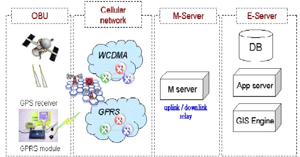
LBS system provides appropriate information service for the users in different locations through the wireless communication network such as GPRS/3G. There are various kinds of LBS applications, for examples, vehicle positioning system (VPS) for electronic toll collection [8], taxi dispatching system (TDS) [12], commercial fleet management systems, and vehicle security systems. The main components of the LBS system (Figure 1) are on-board units (OBU), communication system (cellular network and M-Server), and backend systems (E-Server). OBU is a small computer system which is installed on the vehicle with computing, positioning, communication, and human interface modules. It receives the GPS signal from the positioning module, sending and receiving the messages to and from the backend system through the communication module, and interacts with user via the human interface module. And backend system caches the latest positions and status (e.g. speed, state, etc.) of all the taxies by collecting the uplink reports of OBU. So, the OBU and the backend system interact with each other through the communication system, and they complete the application scenario by complying with the same application protocols.

Figure 1. Components of LBS application

The model proposed by this thesis is using vehicle-based method, which is cost effective without spatiotemporal coverage problem as stated above. This is because the traffic information is derived by data mining from the raw data of LBS, without any additional cost comparing to traditional vehicle-based TTP. Meanwhile, the size of the LBS fleet has the temporal and spatial coverage advantages. Traffic information can be dynamically gathered in the fleet operation area of LBS and 24 hours per day in real-time. The vehicles of LBS applications are regarded as the traffic status probing vehicles of the road network. A vehicle in the LBS application is equipped with an OBU, which has GPS (Global Positioning System) positioning module and wireless communication module such as GPRS or 3G. OBU collects vehicle position, traveling direction, and speed from the GPS module and then uplinks the vehicle status to the backend system through communication module.

The raw data collection is the uplink and downlink interaction logs between OBU and LBS backend system. There are three kinds of uplink logs: periodically report (on

fixed time interval), cross boundary report (on taxi drive through the geographical boundary), and event report (on status change or event happens). The messages of uplink report packet (referred as URP) include current location, direction, speed, and other business-related messages of the taxi fleet vehicles. By combining the road network database in GIS, the traffic information can be collected in real-time by transforming the vehicle status into traffic information of the link that the vehicle located [19]. The transferring function of coordinate address in the GIS engine transforms GPS position of the vehicle into the nearest address by interpolating the GPS position with the road network database. The traveling speed of the vehicle at that address can be a sample of real-time traffic information at the link. Then, the real-time traffic information of the road network can be generated by transforming all the uplink packets in the backend system of LBS.

3.2. Historical Traffic Patterns

After deriving traffic data from LBS, there may exist some embedded traffic information can be applied in various research domains, especially for our TTP expert system. In general, actual TTP has a time lag as it takes a vehicle to travel the whole distance before the actual travel time can be known. Hence, when the actual travel time is measured, the information maybe not in current traffic state to transmit to users. Ideally, when the travel time information is provided, it should be the travel time that the drivers are encountering during their trips. A general method used to estimate current travel time is by summing the travel time derived from speed measurements at different sections of the road simultaneously. The assumption of instantaneous TTP is that present traffic conditions are operative for vehicles entering the road section. This assumption is valid only in free flow condition but as congestion starts building up, the

instantaneous travel time starts lagging. Needless to say, the real-time TTP system is not suitable for predicting at a longer time horizon of saying 1 hour. In addition, our real-time TTP is based on the 24 hours online system, and sometime the probing data will occasionally breaking when probing vehicles entering the tunnel or elevated road to result in losing the important real-time traffic information. Or perhaps, some probing vehicles are not entering in target links (separated by suggested paths of system output). Therefore, there is an urgent need to predict travel time based on historical databases in combination with similar traffic patterns or statistical techniques as well as the real-time traffic information consideration.

Chapter 4 Knowledge-based Travel Time Prediction

The knowledge based real-time TTP model is proposed for travel time prediction in this chapter. There are four phases to achieve the TTP goal: traffic information generation, traffic patterns mining, rules construction, and travel time prediction. In the following sections, the system architecture of our TTP model in the first section is introduced, and the following four sections give detailed discussion of the four phases in this model.

4.1. System Architecture of Travel Time Prediction

In the real life, there are some non-traffic as well as traffic factors which have some impacts to make travel time more unpredictable, such as events, weather, accidents, etc. In order to take these factors into consideration for higher precision of real-time TTP, we propose a real-time knowledge based TTP model to predict travel time. There are two categories in the TTP rules: (a) general rules for real-time and historical TTP are generated from the traffic patterns, (b) meta-rules for tuning the weight of real-time and historical TTP combination ratio are extracted from the human experts.

The basic idea of the model is that travel time can be estimated by using the linear combination of historical and real-time TTP with intersection delay, as shown in (1), where Origin (O), destination (D) and journey start time (t) are the input parameters of the prediction formula, Tc and Th are the sub-functions of real-time and historical TTP results,

and Td presents the intersection delay of each consecutive links, α, β are the weighted

1

)

1

...(

)

,

,

(

)

,

,

(

)

,

(

)

,

,

(

=

+

+

⋅

+

⋅

=

β

α

β

α

where

t

D

O

T

t

D

O

T

D

O

T

t

D

O

T

_{c h d}

In the road network of urban area, an OD pair may have many path choices, and each path consists of several road links. There are many strategies for choosing paths, such as shortest path, expressway first, etc. In this thesis, we adapt the selection scheme of taxi driver’s candidate path, which is discussed in section 4.5. Once the path is decided, travel time along the selected path can be predicted by summarizing travel time of the links in the path and the delays between consecutive links. Assume each Li represents a link in the

selected path: P(O,D), αi, βi are the weight control variables of the link Li, and Di,i+1

presents the intersection delay between link i and i+1. We have the following equation:

i

where

D

t

L

T

L

T

t

D

O

T

i i D O P L i i D O P L i h i i c i i i

∀

=

+

+

⋅

+

⋅

=

∑

∑

∈ ∀ + ∈ ∀

,

1

)

2

...(

)

)

,

(

)

(

(

)

,

,

(

) , ( 1 , ) , (

β

α

β

α

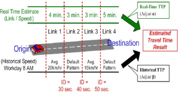
As shown in Figure 2, the users’ vehicle starts from origin site to reach the destination site, and the path is a candidate path obtained by our TTP system, will be separated to consecutive links. In upper part of Figure 2, the real-time TTP of each link is estimated according to its average flow speed. Thereafter, historical TTP of each link is inferred by the rules transformed from historical traffic patterns. Once there is no similar historical traffic pattern, the TTP system use the default patterns which are default values depending on the attributes of links, such as elevated road, main line, second main line, etc.

Figure 2. Linear Combination of Real-Time and Historical TTP

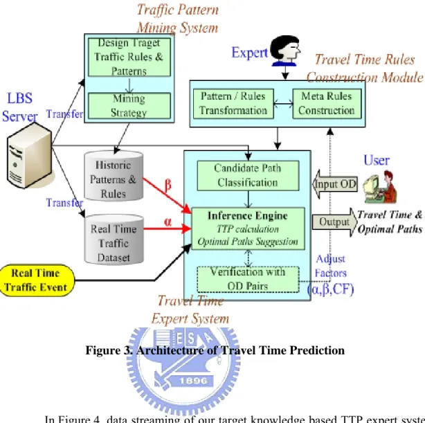
The architecture of TTP expert system contains three modules: traffic pattern mining system (TPMS) module, travel time rules construction module, and travel time expert system module, as shown in Figure 3. The highlight of two red thick lines with α and β combinative variables are obtained from real-time and historical traffic database. After transferring some traffic data from LBS server, we define some target traffic rules and patterns, and then use some data mining strategy to discover the traffic rules and patterns in the TPMS module. Second, in travel time rules construction module, human experts construct meta-rules and transform some traffic patterns into travel time rules which were mined before at TPMS module. For TTP attributes, we build the knowledge classes in travel time rules construction module. Module three presents inference engine of TTP expert system, which computes TTP according to the users’ OD pairs and the candidate path. The verification is also an important subtask of module three, which adjusts α, β, and certainly factors parameters by the past records. The records contained taxi driver’s travel time with equal OD pairs in past. The detail of the above tasks will be discussed in later sections.

Figure 3. Architecture of Travel Time Prediction

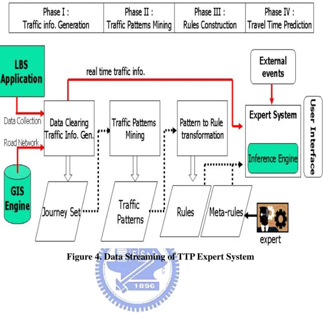
In Figure 4, data streaming of our target knowledge based TTP expert system consisting of four phases including traffic information generation, traffic patterns mining, rules construction, and travel time prediction is proposed. The main distinction can be observed from Figure 3 in Phase I, which is a data preprocessing task for generating our TTP application from LBS server. (Because there involve some meaningless dataset in the original LBS server, and need to be pruned out for our TTP application.) And in Figure 4, two information flows including real-time information flow and batch running historical information flow are highlighted by solid and dotted line respectively.

4.2. Phase I: Traffic Information Generation

The phase I is traffic information generation, including processes of data collection, preprocessing, and transformation from LBS. The process is first creating journey table and traffic information spot (TIS) table schemas, which are derived from LBS, and cleaning some useless raw data to make our probing data more robust (accurate). At last, some categorized traffic patterns in spatial and temporal dimension is defined for storing the results of traffic patterns in the historical traffic database.

4.2.1 Table Schema Derived from LBS

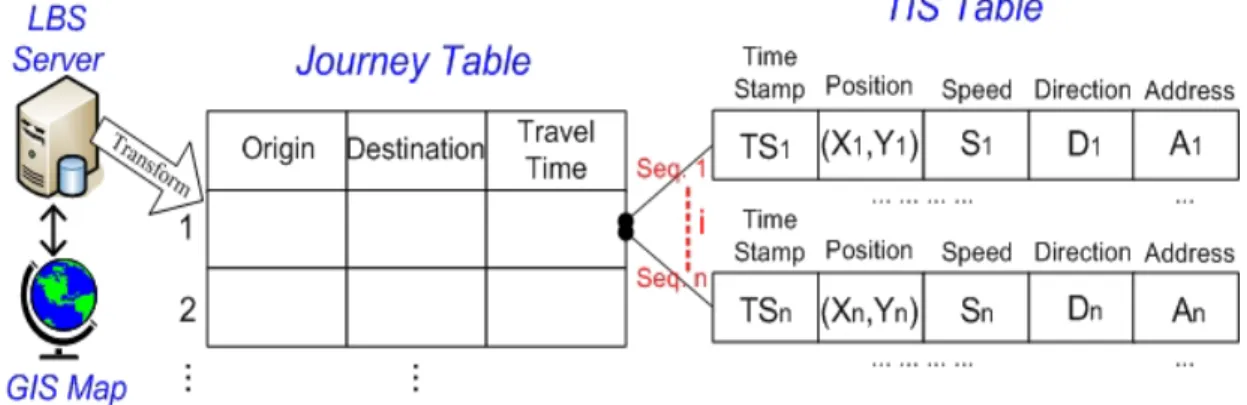
After collecting the raw data of LBS server, data transformation process including three steps is applied to generate the traffic information, as shown in Figure 5. The first step is journey selection, which filters out the meaningless raw data and generates the journey tour of each taxi. There are two cases in a journey of a taxi, one is the tour from dispatched state to occupied state, and the other is the tour from occupied state to the empty state. The former means taxi driver is dispatched to serve the customer, taxi goes from the current location to the customer’s location. The latter means the journey from the customer get on the taxi to the customer’s destination. After journey selection, we can build the OD (Origin and Destination) table, called journey table, as shown in Figure 5. The journey table is a table storing the touring records, where each tour contains one OD pair and a sequence of several URP of the same OBU. These sequences will be stored in TIS table, as shown in the right side of Figure 5. The definition of URP is : URPi = (TSi, (Xi,Yi), Si, Di, Ai), where TSi is the timestamp of the URP, (Xi,Yi) stands for the coordinates of the vehicle, Si and Di are speed and direction of the vehicle, and Ai means

The second step combines the road network data and GIS engine to transform the locations of the URP into real address, which helps mapping the vehicle traveling status to the traffic status of relative road section. Finally the third step summarizes all URP in the journey table of a same temporal section to get average speed of each road section.

As discussed above, the two generated table schema will be used to analyze by data mining technique for producing the historical traffic patterns and rules, and the detail will be introduced in the following sections. By the way, raw data is collected from LBS in real-time at Phase I, and each collected records from LBS application represents location, speed, direction, and status of a vehicle at somewhere the OBU reports to the backend. Hence, we name the real-time location information as traffic information spot (TIS) and create the third table schema for real-time traffic consideration, which is so called real-time traffic spot table. At meanwhile, the traffic information generation process is done at the same time, and the GIS engine [21] helps to convert the coordinates of the vehicle location into address. The speed of the vehicle can be regarded as a sample of each link. The generated traffic information will send the real-time road network status to the expert system, and this information is the inference data source for real-time TTP.

4.2.2 Data Cleaning

After creating our journey and TIS table, we find some noise raw data which are useless, e.g., invalid values of GPS position, speed, and directions, need to be removed from the sequences of TIS table.

Missing values: There are some links of which probing vehicles do not record the

traffic status information. The problem could be caused by GPRS communication or GPS errors. GPS errors might occur when a probing vehicle passes under an infrastructure such as tunnel or the vicinity of elevated structures (the so called urban canon). GPRS communication might be the same reason or any unknown events to cause missing values.

Useless data: In the content of URP, probing vehicle’s speed is 0 in the same

position with a long time. The reason of this happening is probing vehicles were stopping in the ranking station and waiting for servicing. This is because the LBS based probing vehicles are commercial taxi fleet and have “taxi behaviors” on their operating.

Redundant: Some reports of URP show the same message from the same vehicle.

This is because there were several events happened immediately, such as periodically report event after the cross boundary event. So, the reports of message are counted twice and need to be pruned.

4.2.3 Spatiotemporal Traffic Patterns Classification

In this section, we give the definition of spatial and temporal dimensions in order to present our traffic rules and patterns. Classifying the traffic patterns is beneficial to our TTP expert system, but it may have some drawbacks in other situations. The benefit is effective to reduce the computation time on classified historical database, so that only similar segments of the historical database are searched [2]. But, if the searching window time is too large, the real-time online TTP system will be suspended. For example, holiday traffic patterns may be different from the other days of the week. Therefore, predicting the travel time on Sunday can be done by only searching all historical traffic patterns on Sunday in one year. As a result, prediction time can be reduced to 1/7 * 365 (7 days a week). The drawback of classifying the traffic patterns is pattern matching problem, because the fluctuation of TTP is affected by many inferences factors, such as incidents, weather, and driver behaviors. But it is doubtful about only using historical traffic patterns to predict real-time travel time. Here, we give some flexible solutions to handle this problem. Solution one uses dynamic variables of α and β to compute the real-time and historical TTP. Solution two uses the designed TTP system to mine some historical traffic patterns (holiday, working day, etc) which are cleaner without any noise factors (raining, accidents, etc). The system will trigger the meta-rules to dynamically control α and β variables when there are some traffic events on the links for achieving higher accuracy TTP.

The classification method in temporal dimension was grouped into “Year”, “Season”, “Month”, “Date”, “Hour”, and “half an hour” in nature way, and spatial dimension was defined as “City”, “Zone”, and “Road section”. Because the limited speed of Taipei Metropolitan Area is 40 km/hr, we classify 9 fuzzy traffic level statuses.

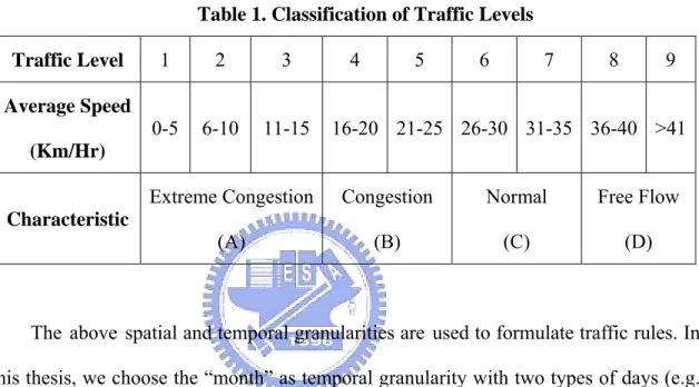
The average speed of collected records between 0-5 km/hr is defined as level 1 and 6-10 km/hr is level 2, as shown in Table 1. We also define some characteristics for traffic status, such as “Congestion (B)” means the average speed falls below 25 km/hr, and if the average speed is below 15 km/hr, called “Extreme Congestion (A)”. “Normal (C)” is the average speed falls between 26~35 km/hr. “Free Flow (D)” is above 36 km/hr,

Table 1. Classification of Traffic Levels

Traffic Level 1 2 3 4 5 6 7 8 9 Average Speed (Km/Hr) 0-5 6-10 11-15 16-20 21-25 26-30 31-35 36-40 >41 Characteristic Extreme Congestion (A) Congestion (B) Normal (C) Free Flow (D)

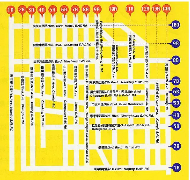
The above spatial and temporal granularities are used to formulate traffic rules. In this thesis, we choose the “month” as temporal granularity with two types of days (e.g. workday and holiday) for calculating the interesting values (e.g. support, confidence). As in spatial granularity, the “road section” granularity is considered in the target area. And the target area of this thesis focuses on the arterial roads of Taipei urban area, as shown in Figure 6.

Figure 6. Road Network in Taipei Urban Area

4.3. Phase II: Traffic Patterns Mining System

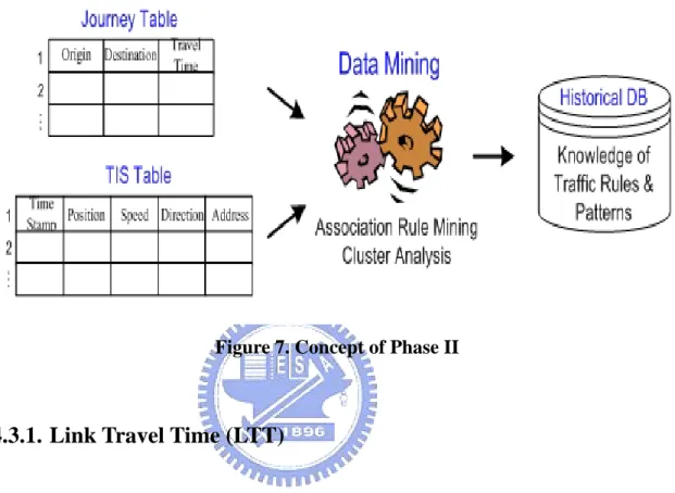
After finishing traffic information generation in Phase I, the traffic information of journey tables are generated and used to discover traffic rules and patterns by data mining technology in phase II, as shown in Figure 7, where the mining results are stored in historical traffic database. There are two types of traffic patterns: link travel time (LTT) and intersection delay (ID). The LTT traffic patterns are used for computing travel time on the target link and the ID traffic patterns are used for predicting intersection

delays of consecutive links. Combining these two types of traffic patterns could generate the historical TTP results and these patterns are discussed in the following sections.

Figure 7. Concept of Phase II

4.3.1. Link Travel Time (LTT)

This section discusses some traffic rules and patterns, which display

the

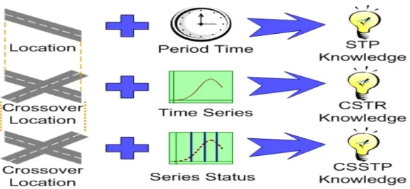
traffic congestion levels and the relationship of spatial and temporal dimensions in traffic network. The influences of traffic network may cause traffic flow to raise the delay of vehicles. Also, LTT traffic patterns are the main component to produce our historical TTP. As shown in Figure 8, there are the three knowledge patterns of LTT: Spatial and Temporal Patterns (STP), Crossover of Spatial and Temporal Rules (CSTR) and Crossover of Spatial and Series Temporal Patterns (CSSTP).

Figure 8. Concept of Three ITT

Spatial and Temporal Patterns (STP)

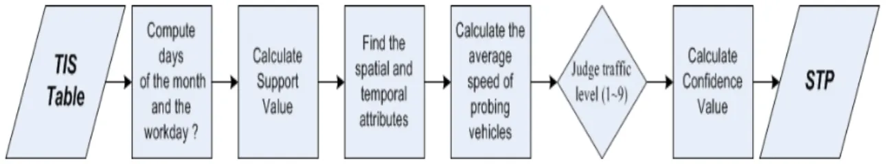
The first knowledge of LTT presents about the traffic condition between time and location as shown in top of Figure 8. We denominate this kind of pattern as “Spatial and Temporal Patterns“. The STP is mined from historical traffic database by aggregating the TIS table in spatial and temporal dimensions. Support and confidence of each STP are determined by calculating numbers of days and times of each traffic levels in every time interval. Spatial dimension stands for the link identification attribute, and temporal dimension is the classified index of time domain. The classified temporal dimension categories include peak or off-peak hour, and holiday or workday, etc. Congestion level, support and confidence can be calculated by aggregating the TIS table in the same spatiotemporal conditions. The STP flow chart is shown in Figure 9 and the format of STP is listed in (3). The Time index are 1~48 and each for half hour of 24 hours a day. If today is holiday then the holiday slot is 1, but for workday is 0. Loc. is road section, Dir. is vehicle’s direction, and traffic level stands for congestion level ranged from 1~9, respectively.

Figure 9. Flow Chart of STP

[Example of STP]

Considering 8 AM Monday (office day), support value on July 2005 (31 days) is (21/31)*100%= 67.74%. The confidence value is concerned the traffic condition of objective location. If congestion occurred in workday 18 times during that month, then the confidence is (18/21)*100%= 85.71%. From above discussion, the meaningful STP is:

STP-(Date, Time index, Holiday, Loc., Dir., Traffic level, Support, Confidence)..(3)

Î (Mon., 16, 0, FuXing S. Sec. 1, ↑, 4, 67.74%, 85.71%)

Traffic status is in congestion.

Additionally, STP are stored in the knowledge class, and can be easily transformed into rules for the TTP inference at run time by combining the link attribute in table of traffic network. The congestion level can be transformed into estimated traveling speed on that link, and thus the estimated travel time can be calculated by dividing the length of the link with the estimated speed.

Crossover of Spatial and Temporal Rules (CSTR)

The second LTT knowledge is used to find the traffic information of crossover road sections, which consists of two space dimension and one time dimension. So the name

of this knowledge is “Crossover of Spatial and Temporal Rules”. The CSTR is generated by integrating two traffic sequences of the crossover road sections. The correlations between two crossover road sections may be independent with each other. Thus, what correlation (positive or negative) in the target crossover is concerned? If positive correlation, it means that the traffic flows of vehicles’ directions on the former road section has a tendency to drift towards the latter road section. This is called as “transmit probability” on this intersection. According to the CSTR knowledge, we can understand the impaction of congested vehicles, and realize the drivers’ behaviors that they used to route. The correlation value between two road sections can be calculated as follows (4).

Correlation = P(A)^P(B) / P(A)P(B) …(4)

Here the equation, P(A)^P(B) = P(A)*P(B), means traffic sequences of two crossover road sections (A and B) are in congested status in the same time interval. Also, support values in CSTR are calculate by P(A)^P(B). The CSTR flow chart is shown in Figure 10. The first process executes to encode the sequence patterns of the target direction road sections. If average speed of road section is below 25 km/sec, encode 1 (Because we are interested in congested status). Higher the average speed 25 km/sec is encoded 0. After this transformation, the road section congestion sequence can be generated. Then, the computation of correlation values of crossover sections can refer to the equation (4) for generating CSTR. Thus, if A and B is negatively correlated, then the result of correlation value is less than 1.

[Example of CSTR]

Considering two STP on Monday of FuXing S. Sec. 1 (↑) and RenAi Sec.3 (Æ), we encode the average speed in binary code with half hour interval from 6 AM to 11 PM, as following:

FuXing S. Sec. 1 (↑): 00111 10101 11111 11011 11111 11111 1110 RenAi Sec.3 (Æ): 00011 11111 11111 00001 10011 11110 1100

Then, the support value is 20/34 = 0.5882, and correlation value is 0.5882 / (22/34) * (28/34) = 1.104 that calculated be equation (4). From above discussion, the meaningful CSTR is:

CSTR-(Date, Holiday, Location, Direction, Support, Correlation) … (5)

Î (Mon., 0, FuXing S. Sec. 1, ↑)

^

(Mon., 0, RenAi Sec. 3 , Æ)

It’s positively correlated congestion in this crossover, Sup.= 58.82%, Corr.= 1.104

Figure 10. Flow Chart of CSTR

Crossover of Spatial and Series Temporal Patterns (CSSTP)

The third LTT knowledge: CSSTP, which is shown in the bottom of Figure 8. The main difference motive between CSSTP and CSTR is, “how long the traffic condition status will continue?” In other words, the CSSTP can find out a period of time that the congestion status will continue on crossover road sections, or it is just a short period phenomenon. This knowledge patterns can provide more useful information for the

traffic center manager, and help them to do some actions for improving the traffic flow. The name of this knowledge patterns is called “Crossover of Spatial and Series Temporal Patterns” (CSSTP). The format (6) and a CSSTP record are listed below:

[Example of CSSTP]

CSSTP-(Date, Time index start, Time index end, Holiday, Loc.1 Dir., Loc.2 Dir., Traffic level, min. Sup., min. Con., min. Corr.) …(6)

Î (Mon., 16, 19, 0, FuXing S. Sec. 1 (↑), RenAi Sec. 3 (Æ), 4, 60%, 80%, 1.1)

Traffic status is congestion in this crossover from 8AM to10AM.

In CSSTP, the ARCS (Association Rule Clustering System) [9] technique is applied to find out the continue traffic condition (e.g. congestion) of CSTR. As the flow chart of Figure 11, first, ARCS use the binning method to replace the data of attributes (e.g. space, time) with their corresponding bin number, and segmentation criteria separate every crossover road sections of CSTR into parts by human expert.

In association rule engine of ARCS, we recomputed support and confidence of CSTR in order to compare the min. support and min. confidence of the heuristic optimizer. Then, we transform these association rules into two dimensions bitmap and use grid clustering technique to find out the temporal continuity of the traffic condition in the same crossover road sections. The bitmap clustering is shown in Figure 12.If the association rules of CSTR are corresponding to threshold of min. support, min. confidence and min. correlation, it will encode “X” on the bitmap. Then, the Euler formulation is used to compute the distance in grid map for clustering the nearest grids. The clustering mechanism may extend the temporal dimension of traffic levels and group them together. (Here, we consider the time dimension). Thus, the results of these groups are regarded as CSSTP. In order to make CSSTP more accurate, the clustering analysis is verified with test data, and use heuristic optimizer to adjust the parameters (e.g. min. support, min conf., min. corr.) in loop procedure. Finally, more accurate results of CSSTP can be generated after the loop process of ARCS.

Figure 12. Bitmap clustering of CSSTP

4.3.2. Intersection Delay

mostly caused by signal delay and queuing delay. Estimation of the intersection delay is too hard to be defined by mathematical model; thus many past researches just give a default values as a solution. However, in urban traffic network, there are too many intersections and each of them has different signal delay (arterial road may have more time slot). Here we proposed two ways to estimate the intersection delay: traffic patterns and meta-rule from expertise. Traffic patterns related to intersection delay can be classified by Through Delay (TD), Left Turn Delay (LTD, as Figure 13) and Right Turn Delay (RTD), which are the delays of three possible directions from one link connect to another link, and can be extracted from the historical journey set of traffic database. In general, TD might be caused by traffic signals of red light or none by green lights. Here, we adopt average TD values for TTP system. The LTD might be the largest average delay value of these three kinds intersection delay, because it combines signal time and queuing time as shown in Figure 13. And normally, RTD is the lowest average delay value in this research.

Figure 13. Example of LTD

Equation (7) shows the general format of TD/LTD/RTD, where P is the pattern type (0-LTD, 1-TD, 2-RTD), SOid and SIid are the two consecutive links ID where

T is the temporal index (0-nonpeak hour, 1-peak hour, 2-default), and Davg is the

average delay time of this pattern.

[TD/LTD/RTD] : (P, SOid, SIid, Tid, Davg) … (7)

Intersection delay pattern can be aggregated by consecutive two TISs with different links in the historical journey set table. Figure 14 shows an example of RTD pattern: a probing vehicle drives on north direction then turn right to east, and report TIS at location A of Link La and consecutively report TIS at location B of Link Lb. The

symbols of the TIS format (T,L,X,Y,D,S) in Figure 14 stand for timestamp (T), link id (L), coordinates (X,Y), direction (D) and speed (S) respectively. The distances da and db

in Figure 14 stand for the distance from A, B to the intersection of links La and Lb

respectively. The right through delay time from the La to Lb can be estimated by

subtracting travel time of da and db from elapsed time between two TIS, A and B. To

sum up, the flow chart of intersection delay is shown in Figure 15.

Intersection delay can be easily estimated by another strategy expert heuristics. Average delay value in the rule of TD/LTD/RTD for each consecutive link is extracted from human experts and stored in the knowledge base. The experiments will compare traffic pattern and expert heuristic strategies to find out which one has better results.

Figure 15. Flow Chart of Intersection delay

4.4. Phase III: Meta Rules and Knowledge Class

The concept of Phase III, as shown in Figure 16, discusses about the interferences (attributes) of TTP and the building of knowledge class for later TTP expert system. Also, the transformation of the results of traffic patterns (ID and STP patterns) from Phase II into travel time rules will be described. The construction of meta-rules, which can dynamic control the variables (αandβ) on the travel time rules of the historical and real-time travel time estimations, will be discussed at last.

Figure 16. Concept of Phase III

4.4.1. Interferences and Attributes of Travel Time Prediction

As shown in Figure 16, the vehicle starts at an origin position to reach its destination has many attributes for computing our TTP, and some of these attributes (facts) are regarded as interferences, which might delay the vehicles to reach the destination. Here, we list and briefly describe all attributes of TTP. First, Time and

Location are not only the important index to present traffic information but also the

basic materials to formulate our traffic patterns and travel time rules. As we mentioned above, in this thesis, 1~48 time index to present 24 hours a day: 1 present 00:00 to 00:30, 2 present 00:30 to 01:00 and so on. The Location in this thesis is considered road sections in Taipei urban network as Figure 6, such as the sections of Zhong Xiao East Road. The Direction of LBS-based vehicles is also an attribute of TTP. Then, after considering time and location facts, the most important fact is Traffic Status, which has level 1-9 of average traffic speed. Then, we use the above facts to construct our STP knowledge.

In TTP, some geometry information is necessary material, such as Road Length and the Coordinates (X, Y) of intersection in GIS map. Because system can not compute the link travel time when it has the average speed in the target road but do not know the length of road. Thus the length of each section (Link) is needed in our target urban network. The coordinates (X, Y) of intersection are referred to GIS map and GPS position. These longitude and latitude of intersections are necessary for TTP system to precisely compute the ID patterns. The default patterns are used to handle missing or no related historical patterns (STP) in historical database. According to the Directorate General of Highways, we use some classified roads for making our default pattern. For example, the speed limit of freeway is 100KM/HR and second main line of urban network is 40KM/HR, etc. Then, TTP system can use this limit speed and the length of road to compute link travel time. Real-Time Events are the significant interferences of TTP. Here, we take incidents, road constructions and heavy raining events into account.

Types of Day, such as holiday and workday are also considered. Because different

traffic flows in the traffic network will have different traffic patterns, and we need to separate it for making our historical TTP more accurate. At last, Meta-rules and

Knowledge Class of traffic patterns (STP, ID patterns) are also the portions of our TTP

considerations, which will be discussed in following sections.

4.4.2. Generation of Travel Time Rules

After data mining process in Phase II, the three knowledge traffic patterns were found. Some of them are meaningful in TTP but some are not. In our goal of TTP expert system, we only use the STP knowledge and transform it into knowledge class [13]. Because, STP knowledge can be easily transformed into travel time rules for the TTP inference at run time by combining the link attributes in the road network table. Also, the

intersection delay patterns will be transformed into knowledge classes. And these knowledge classes can be used in the inference engine of TTP expert system at Phase IV. Here are some transformation examples of STP and ID patterns as shown below.

„ STP to Travel Time Rules

STP- (Date, Time index, Holiday, Location, Dir. , Traffic level, Sup., Conf.) Here, we assume min. sup. =0.7, min. con. =0.8,

Ex: STP - (1, 16, 0, A1, 1, 4, 70%, 85%)

→ If Workday & 8am & A1 E. , then traffic level 4 …… (Travel time rule)

First, according to STP format in (3), time index, holiday, location, direction, and traffic level are chosen to transform the STP into travel time rules. Then, the “if… then…” style is used to formulate our target travel time rules. The fact in RHS of travel time rules is only the traffic level, and the remaining facts are in the LHS of travel time rules. The thresholds of minimum support and minimum confidence are given by human expert for making our travel time rules more robust.

The transformation of ID patterns can refer to the format of ID patterns as (6). Every slot of ID format can be used to formulate travel time rules, where the fact in RHS of travel time rules is only the delay value and the other facts are in the LHS of travel time rules. The example is shown below:

„ ID Patterns to Travel Time Rules [TD/LTD/RTD]: (P, SOid, SIid, Tid, Davg)

4.4.3. Meta Rules Construction

The meta-rule is designed as a reaction mechanism to the current external traffic or non-traffic events in order to raise the precision of the real-time TTP in this section. In equation (1) and (2), control variablesαandβrepresent the weight of real-time and historical TTP respectively. Meta-rule, which is extracted from the expert, is the tuning mechanism for weighted combination of real-time and historical TTP. That is, meta-rules dynamically tune the value of weight control variables:αandβ. For example, if system receives a current external event, such as car accident on a link in the selected path, meta-rule mechanism will then reduce the weight of historical and raise the weight of real-time TTP. Because the effect of that car accident can reflect at that link immediately, so raising the ratio of real-time TTP can get higher precision. Here, the meta-rule is shown below and the style of meta-rules is as same as “if… then…” format of travel time rules. In addition, the initial values of αandβ are given by human expert. In order to emphasize the real-time traffic status is more important in our real-time TTP system, the initial value ofαandβare set 0.7 and 0.3 by human expert, respectively.

[Meta-Rule]: If link is under construction, then α+=0.05 , β-=0.05

On the other hand, some meta-rules may raise the weight of historical TTP in several conditions: One, if there is no event happening or lacks real-time traffic information of LBS-based vehicles, Two, if the support and confidence values of the related traffic patterns (mining from the historical database) are higher than the thresholds. It means that there is a strong support that traffic status is possible to regress to the intents of related historical traffic patterns. Therefore, raising the weight of

historical TTP might get higher precision of TTP. The general format of this type meta-rule is like:

[Meta-Rule]: If link covers fewer probing vehicles, then α-=0.05 , β+=0.05

4.5. Phase IV: Travel Time Prediction

In Phase IV, the TTP calculation of our knowledge-based expert system will be described. At first, when user gives the OD pair, TTP expert system uses this OD to output some suggested paths with travel time results for user. But, how these paths are generated for TTP expert system? And what are the procedure and reasoning step in inference engine for producing the travel time results with these paths? These questions will be discussed in later section.

4.5.1. Candidate Paths Generation

The TTP expert system contains some well solutions (shortest paths), which are corresponding to users’ given OD pairs to output for users. If there are no well paths in TTP expert system, calculating TTP results is in vain. However, the path selection problem in the urban road network is more complicated than in freeway. There are fewer path choices in freeway routing if the OD pair is given. But in urban network, there is a combination explosion problem. There are many strategies for path routing on a given OD pair in the urban network, such as shortest path first, expressway first or signal less path first, etc. The path selection problem is beyond the scope of this thesis. Fortunately, LBS application gives a statistic solution here. The drivers (such as taxi

tend to select heuristic paths depend on their experience and the traffic status. So the candidate path classification subtask of travel time expert system module in Figure 3 is implemented according to this concept. Top 3 paths will be selected from the journey set in the historical traffic database as the candidate paths, and each one of them will be evaluated to decide which path is the suggested path, which will be discussed in later section. The flow chart of candidate paths generation is shown in Figure 17. In this Figure, it uses the journey table and TIS table as data sources, then according to the classified OD pairs to do the statistic process for computing top 3 candidate paths. Finally, TTP system will store these candidate paths in database with human expert for later querying.

Figure 17. Flow Chart of Candidate Paths Generation

4.5.2. Suggested Paths Generation

After generating the candidate paths, TTP system has many candidate paths of each OD pairs. However, the urban traffic network in Taipei is complex and OD pairs might have many combinations of user’s demands (different origins with different destinations). So, here we just assume our candidate paths generation can cover all

users’ demands. On the other hand, these candidate paths are generated by taxi driver’s experience, as we mentioned above. But there still are some disadvantages of these candidate paths. Although the taxi drivers have their experience paths in mind to take passengers to their destination, their “experience shortest paths” may be not the optimal paths in current traffic status. Besides, when taxi drivers were driving their cars, they did not understand the traffic events or congestion links were happening on their experience paths during their trips (seldom of taxi drivers were hearing the traffic reports on radio). Thus, using the statistic process to generate some candidate paths on their experience paths still needs to optimize these paths with current traffic status (such as real-time events or link traffic levels). In this section, the optimized procedure in our designed knowledge based TTP expert system will be described. The concept of our TTP expert system is shown in Figure 18. In this Figure, the input data are OD pair with time, and output data is TTP with suggested paths. The inference engine will use knowledge classes of ID patterns and STP with some auxiliary documents, such as road geometry (length of road sections), meta-rule, default patterns, candidate paths and external real-time events, to compute the real-time and historical travel time.

The procedure of knowledge based TTP expert system is shown in Figure 19. At first, the expert system uses the given OD pair with current time to search the candidate paths, and decomposes these paths to links in order to calculate travel time in each different traffic levels. Then, inference engine of expert system triggers knowledge classes of STP to know the historical traffic level of each links. If link has no corresponding STP, default patterns will be used as the link speed. Later, system uses road geometry document to know each link’s length for computing the historical travel time (divided average link speed). After historical travel time process, the real-time travel time process computes the average speed of each link using the real-time traffic spot schema and collected datasets. Thereafter, system can dynamically set up α and β variables using meta-rules with real-time events and calculate final TTP results for each candidate path. The verification process with OD pairs in dotted line is used for turning robust variables (such as α, β and certainly factors of travel time rules) by journey table’s travel time slots. This verification process has been done during the simulated period.

Chapter 5 Experiment

5.1. System Architecture

The TTP prototype system was implemented based on a real-time LBS: taxi dispatching system (TDS) [12]. The TDS is an online 7*24 system operated in Taipei urban area, and the current fleet size is about 1000 taxis, where the OBU installed on the taxi can report its current status periodically (30 sec), or when some events occur. The events may include spatial trigger event, dispatch/response event, customer on/off taxi events, etc. By translating the OBU reports to TISs, currently the TDS raw data could be half a million TISs per day, and becomes a good data source for this prototype TTP system. At the data collecting and clearing phase, the OBU report raw data has been collected and translated to TIS in a period of 5 minutes in order to catch the real-time traffic information, and all the TISs are filtered out except the OBU being in ‘dispatch’ or ‘occupied’ state since the traffic information extracted from these two states is meaningful. Besides, the OBU report will be filtered out if the location of its TIS is not in the interested links (links in Figure 6). Historical traffic information consisted of journey sets, which are parsed from the raw data by combining the GIS road network. A journey is a tour with explicit origin and destination, and consists of several TISs between origin and destination. For example, ‘dispatch’ state journey starts from the dispatch location to the customer’s location, and ‘occupied’ state journey starts from the customer’s location to customer’s destination.

As shown in Figure 6, the target area of this prototype system focuses on arterial roads in Taipei urban area, and each arterial road may have one or several links. Link attributes are defined and default values are given by domain experts in order to