應用於三維繪圖系統之低複雜度切割演算法與高能源效率幾何引擎設計

國

立

交

通

大

學

資訊科學與工程研究所

碩

士

論

文

應用於三維繪圖系統之

低複雜度切割演算法與高能源效率幾何引擎設計

Power Efficient Geometry Engine Using

Low-Complexity Subdivision Algorithm for 3D

Graphics System

研 究 生：許籐耀

指導教授：范倫達 博士

中 華 民 國 九 十 七 年 十 月

低複雜度切割演算法與高能源效率幾何引擎設計

A Power Efficient Geometry Engine Using Low-Complexity

Subdivision Algorithm for 3D Graphics System

研 究 生：許籐耀 Student：Ten-Yao Sheu

指導教授：范倫達博士 Advisor：Dr. Lan-Da Van

國 立 交 通 大 學

資訊科學與工程研究所

碩 士 論 文

A Thesis

Submitted to Institute of Computer Science and Engineering College of Computer Science

National Chiao Tung University in partial Fulfillment of the Requirements

for the Degree of Master

in

Computer Science

Oct 2009

Hsinchu, Taiwan, Republic of China

應用於三維繪圖系統之

低複雜度切割演算法與高能源效率幾何引擎設計

學生：許籐耀 指導教授：范倫達 博士

國立交通大學 資訊科學與工程研究所

摘 要

在本篇論文中，我們提出了一個低複雜度的三角形切割渲染演算法與具有高 能源效率的幾何引擎架構。所提出的切割演算法與架構能提供近似馮氏渲染的繪 圖品質，同時能藉由調整切割層級達到有動態調整繪圖品質與功率消耗的能力。 目前可支援三種不同層級的切割模式。 本文所提出的幾何引擎架構運用了數項不同的技術來對功率消耗、效能、面 積進行最佳化。例如使用所提出的前向差分切割、邊函數修正、雙空間切割、三 角形濾除與頂點快取記憶體等技術可以有效減少幾何轉換與打光運算。針對複雜 的運算，我們提出了可重組的資料路徑架構並藉由將資料路徑重組成特定的結構 來加速複雜運算的處理。由於重組架構使用相同的硬體進行不同的運算，晶片面 積與成本也能有效的減少。與傳統的切割式渲染演算法相比，分別對於一層與兩 層的切割渲染運算，我們提出的方法可以減少記憶體存取次數達 44.44% 與 68.88%，同時幾何轉換乘法運算量也能分別減少 50% 與 80%。此設計已使用 UMC 90 奈米製程實現，從晶片模擬結果顯示 我們所提出幾何引擎可以達到 16.978 MVertices/(smW)之高能源效率。

A Power Efficient Geometry Engine Using

Low-Complexity Subdivision Algorithm for 3D

Graphics System

Student：Ten-Yao Sheu Advisor：Dr. Lan-Da Van

Institute of Computer Science and Engineering College of Computer Science

National Chiao Tung University

ABSTRACT

In this thesis, a power efficient geometry engine (GE) using a low complexity three-level subdivision algorithm is presented. The proposed subdivision algorithm and architecture is capable of providing low power, scalable and near-Phong shading quality. The forward difference, edge function recovery, dual space subdivision, triangle filtering schemes and post-TnL vertex are employed to alleviate the redundant computation for transforming and lighting of the proposed algorithm and architecture. Due to the three-level subdivision algorithm, one reconfigurable datapth is proposed to reduce the area since the same set of processing elements (PEs) is reused for different operations for the GE. Compared with the conventional subdivision algorithm, the reduction of the number of memory accesses can be attained by 44.44% and 68.88% for level-1 and level-2, respectively. The reduction of the number of multiplications for transforms can be attained by 50% and 80% for level-1 and level-2, respectively. From the implementation results in UMC 90nm, the proposed geometry engine can achieve

誌 謝

感謝指導教授范倫達老師。在碩士班這段時間老師提供了我各方面的協助， 也花了很多時間審查我的論文和思考改進我的研究，使我可以確立並完成我的論 文研究，讓我在研究所的期間收穫豐碩，因此在這邊對老師表達由衷感謝。同時， 亦感謝周懷樸教授、陳紹基教授、簡韶逸教授三位口試委員給予精闢的審查意見。 其次，我也要感謝 VIPLab 的同學、學長姐、學弟妹們，姵妤學姐，特別是旭 昇學長在 EDA 軟體提供了許多協助，以及同窗迪優、宗哲、宗融、晉豪與得安在 研究上給予我很多建議。最後就是可愛的學弟學妹們丞蔚、思翰、庭維、坤隆、 家育、盈里、建勳、曉霜、家榮、睿峻、泊硯，與你們相處的回憶對我來說都是 相當珍貴的。 最後，我要感謝我的父母親還有祖母，你們是我心靈上最大的支柱，你們的 關心和鼓勵都是我最大的動力來源，你們讓我能順利完成學業和此篇論文，非常 感謝你們。

Contents

摘 要 ... I

ABSTRACT ... II

誌 謝 ... IV

CONTENTS ... V

LIST OF TABLES ... VII

LIST OF FIGURES ... VIII

Chapter 1 Introduction ... 1

1.1 Motivation ... 2

1.2 Thesis Organization... 3

Chapter 2 Proposed Low Complexity Subdivision Algorithm ... 4

2.1 Subdivision Using Forward Difference ... 4

2.2 Edge Function Recovery Scheme ... 8

2.3 Dual Space Subdivision Scheme ... 13

2.4 Triangle Filtering Scheme ... 18

Chapter 3 Proposed Geometry Engine Architecture ... 23

3.1 Primitive Input Control (PIC) ... 24

3.2 Primitive Queue (PQ) ... 25

3.3 Dispatch Queue (DQ) ... 25

3.4 Vertex Cache Management Unit (VCMU) ... 26

3.5 Primitive Processing Unit (PPU) ... 27

3.6 Vertex Processing Unit (VPU) ... 28

3.6.1 Processing Element (PE) ... 31

3.6.2 Special Function Unit (SFU) ... 37

3.6.3 FIFO ... 38

3.6.4 Special Function Unit (SFU) ... 39

Chapter 4 Comparison Results and Chip Implementation ... 45

4.1 Complexity Comparison Results... 45

4.2 Chip Implementation and Comparison Results ... 48

Chapter 5 Conclusion ... 52

Bibliography ... 53

Publication List ... 57

List of Tables

Chapter 2

Table 2.1 Complexity analysis of the eye space subdivision ... 16 Table 2.2 Complexity analysis of the perspective correct dual space subdivision

... 17

Table 2.3 Complexity analysis of the perspective incorrect dual space subdivision

... 18

Chapter 3

Table 3.1 Configuration modes for RDP ... 31

Chapter 4

Table 4.1 Complexity comparison results in general representation between conventional subdivision algorithm and proposed subdivision algorithm. ... 46 Table 4.2 Complexity comparison results for level-1 case (NS = 2, NG = 3, NA = 5). ... 47

Table 4.3 Complexity comparison for level-2 case (NS = 4, NG = 12, NA = 5). ... 47

Table 4.4 Chip characteristics of the proposed GE architecture ... 48 Table 4.5 Comparison results among the existing work ... 51

List of Figures

Chapter 2

Fig. 2.1 Illustration for subdivision using forward difference ... 5

Fig. 2.2 Examples of rasterization anomaly: (a) Teapot, (b) Pawn, (c) Venus, (d) Couch. ... 7

Fig. 2.3 Illustration of the rasterization anomaly ... 8

Fig. 2.4 Illustration of the rasterization anomaly ... 9

Fig. 2.5 Illustration of computing the edge functions for small triangles. ... 11

Fig. 2.6 Rendering results with the proposed edge function recovery scheme: (a) Teapot, (b) Pawn, (c) Venus, (d) Couch. ... 12

Fig. 2.7 Flow chart of the transforms in the geometry engine. ... 13

Fig. 2.8 Data flow of eye space subdivision ... 14

Fig. 2.9 Data flow of dual space subdivision ... 15

Fig. 2.10 Data flow of the triangle filtering scheme ... 19

Fig. 2.11 Illustration of the triangle setup variable sharing ... 22

Chapter 3 Fig. 3.1 Overall architecture of proposed GE architecture. ... 24

Fig. 3.2 Illustration of the dispatch queue ... 25

Fig. 3.3 Illustration of the vertex cache management unit ... 27

Fig. 3.4 Block diagram of the primitive processing unit ... 28

Fig. 3.5 Block diagram of the vertex processing unit ... 30

Fig. 3.6 Block diagram of the processing element ... 33

Fig. 3.7 Illustration of multiplication operation ... 34

Fig. 3.8 Illustration of square operation ... 35

Fig. 3.9 Illustration of MAC operation ... 36

Fig. 3.10 Illustration of addition/subtraction operation ... 37

Fig. 3.11 Block diagram of the special function unit.. ... 39

Fig. 3.12 Interconnection of the transform dp configuration mode. ... 41

Fig. 3.13 Interconnection of the light dp configuration mode. ... 41

Fig. 3.14 Interconnection of the vector normalization configuration mode ... 43

Fig. 3.15 Interconnection of the perspective division configuration mode... 43

Fig. 3.16 Interconnection of the vector subtraction configuration mode ... 44

Chapter 4 Fig. 4.1 Chip layout of the GE. ... 49

Fig. 4.2 Rendering result of different subdivision levels: (a) level-0, (b) level-1, (c) level-2.. ... 50

Chapter

1

Introduction

Nowadays, 3D graphics functions are integrated into the wireless- and wired-multimedia terminals such as mobile devices and 3D TV systems [1]. 3D graphics system is composed of geometry engine (GE) and rasterization engine [2]. In GE, Gouraud shading [3] with per-vertex lighting is widely used because it only applies reflection model [4] on the vertices of the polygons and uses bilinear interpolation to obtain the intensities for the pixels inside the polygons. Although Gouraud shading has less computation complexity than other approaches, it suffers from Mach band effects and produces polygonal highlights on the rendered objects. Phong shading [5] uses bilinear interpolation to obtain the normal vectors for the internal pixels and applies the reflection model on each pixel. Phong shading can produce more smooth and accurate highlights than Gouraud shading. However, it needs to re-normalize the normal vector and computes the light intensity for every pixel inside the polygon. Phong shading possesses high shading quality, but consumes much more power because of the huge computation requirement.

Recently, low computation, satisfactory quality, and power efficiency are the important research issues for hardware design. In order to have near-Phong shading quality with low computation, several approximate Phong shading schemes have been proposed as follows. The Taylor expansion [6] is used to approximate Phong reflection

multi-light sources. Spherical interpolation algorithms [7][8] aim to avoid re-normalizing the normal vectors, but the setup must be performed for each scan line and for each light source. Thus, the setup cost is expensive for thin polygons and the multi-light source scenes. The mixed shading [9][10] combines two shading methods. When the highlight covers the polygon, it is rendered using Phong shading. Otherwise, Gouraud shading is employed. Although deferred shading [2] removes the lighting operations on the hidden pixels, the lighting equation is still applied to the visible pixels. To completely eliminate per-pixel lighting quadratic interpolation, the work in [11][12] uses a quadratic function to interpolate light intensities between six points. The quadratic scheme would incur Mach band effect on the edge if the triangle is too large. Therefore, an error control scheme is proposed in [11] to solve this problem. Subdivision scheme [10][13][14][15][16] is another approach to approximate Phong shading. It subdivides a triangle into smaller ones and renders them individually with Gouraud shading. Compared with other per-pixel lighting approximate schemes, only vertices are lit. One attractive feature of subdivision scheme is its ability to scale shading quality dynamically. If higher shading quality is demanded, more small triangles are generated. Otherwise, fewer triangles are generated to reduce the processing time and power consumption. From another point of view, the power can be used more efficiently if the shading quality is scalable.

1.1 Motivation

Although the conventional subdivision algorithm inherently provides scalable and near-Phong shading quality, the computational complexity and power consumption are still large for GE. Thus, we are motivated to propose a low complexity subdivision algorithm and the corresponding power efficient and scalable-quality geometry engine in the thesis.

1.2 Thesis Organization

The rest of the thesis is organized as follows. The proposed subdivision algorithm and the corresponding complexity analysis are described in Chapter 2. In Chapter 3, the proposed GE architecture is presented. The comparison results and chip implementation are addressed in Chapter 4. Last, a brief statement concludes the presentation of this thesis.

Chapter

2

Proposed Low Complexity Subdivision

Algorithm

In this chapter, a low complexity subdivision algorithm to approximate Phong shading is proposed. To reduce the redundant memory accesses, the forward difference technique is used to subdivide triangles in the proposed algorithm. Since the forward difference technique is numerical instable, there may be rasterization anomalies on the rendered objects. Hence, an edge function recovery scheme is proposed to remove the rasterization anomalies. In the subdivision-based approximate Phong shading algorithm, the increased number of triangles becomes a potential problem to the computation and power consumption. In order to reduce the complexity of the proposed algorithm, the dual space subdivision scheme, triangle filtering scheme and the triangle setup variable sharing scheme are also presented. The proposed algorithm and schemes are described in detail in the following subsections.

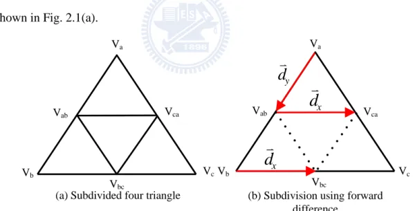
2.1 Subdivision Using Forward Difference

Forward difference [13] method is widely used to evaluate the polynomial function. Herein, use it to reduce the memory accesses for triangle subdivision. An example is illustrated in Fig. 2.1. To subdivide the triangle Δ VaVbVc in Fig. 2.1 (a), the intermediate vertices: Vab, Vbc, Vca are computed. Then these new vertices together with

the original vertices will be packed and new triangles are generated as: Δ VaVabVca,

Δ VabVbcVca, Δ VabVbVbc and Δ VcaVbcVc. These new triangles will be output for next-stage processing. The forward difference method is used to compute the intermediate vertices. The first step is to compute the difference vectors d_x and d_y in horizontal and vertical direction using Eq. (2.1) and Eq. (2.2).

S b c x V V N d ( - )/ (2.1) S a b y V V N d ( - )/ (2.2)

, where NS= 2L denotes the number of the segments on each edge of the original triangle and L is a non-negative integer. Without loss of the generality, we set the NS = 2 as shown in Fig. 2.1(a).

(b) Subdivision using forward difference

Va

Vb Vc

(a) Subdivided four triangle Va Vb Vc Vab Vbc Vca Vab Vbc Vca y

d



x

d



x

d



Fig. 2.1. Illustration for subdivision using forward difference.

Once the difference vectors are computed, the intermediate vertices can be generated by Eqs. (2.3), (2.4) and (2.5) as shown in Fig. 2.1 (b).

y a ab V d

x ab ca V d V    (2.4) x b bc V d V    (2.5)

Computing the intermediate vertices using the forward difference method is more efficient than other methods because generating one intermediate only needs one memory access to store the vertex. Compared with the conventional recursive-based subdivision algorithms [10][13][14][15][16], the forward difference method is stack free and hence the number of memory accesses can be reduced. In other words, the power can be alleviated. However, the subdivision algorithm using forward difference would result in the rasterization anomaly where pixels are lost on the rendered object. As shown in Fig. 2.2(a), (b), (c), (d), the empty pixels on the teapot, pawn, Venus, and couch are the lost pixels. The cause of the anomaly is the numerical instability of subdividing the triangle using the forward difference scheme. An example is illustrated in Fig. 2.3, where two adjacent triangles are subdivided using forward difference. In Fig. 2.3 (a), Vm denotes one intermediate vertex on the sharing edge of two triangles. It can be obtained from subdividing either the left triangle or the right triangle if the calculation has no error. In Fig. 2.3 (a), the vertex Vc is the intermediate vertex in the subdivided left triangle and is computed from the vertex Vb using the difference vector

x

d twice. The vertex Vc has the same coordinate as the vertex Vm if the calculation has no error. However, the calculation has the quantization error such that the vertex Vc has different coordinate from the vertex Vm. For the same reason, in the right triangle of Fig. 2.3 (a), the vertex Vd computed from vertex Va with forward difference vector dy

 has different coordinate from the vertex Vm. As a result, the small triangles defined by vertex Vc and Vd respectively are not adjacent to each other. Fig. 2.3 (b) shows the

rasterization result of the sharing edge. Since the pixels are lost on the sharing edge after rasterization, the rasterization anomaly occurs.

(a) Teapot (b) Pawn

(c) Venus (d) Couch Fig. 2.2. Examples of rasterization anomaly.

Fig. 2.3. Illustration of the rasterization anomaly.

2.2 Edge Function Recovery Scheme

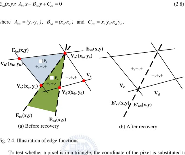
In order to remove the rasterization anomaly, a recovery scheme based on the edge function method is proposed. The edge function method [16] is used in some raster engine to decide whether a pixel is in the triangle. The edge function is a line equation through the two vertices of the triangle edge. For example, in Fig. 2.4 (a), the edge function Eab of the left triangle defined by vertices Va and Vb is expressed in Eq. (2.6), where (xa, ya) and (xb, yb) are the coordinates of vertex Va and Vb.

0    _{ab ab} ab ab(x,y): A x B y C E (2.6) where Aab (ya-yb), Bab (xb-xa) and Cab  xayb-xbya.

The other two edge functions Ebc and Eca can also be similarly derived as follows.

0    bc bc bc bc(x,y): A x B y C E (2.7) where A_bc (y_b-y_c), B_bc (x_c-x_b) and C_bc  x_by_c-x_cy_b. (b) Rasterization result (a) After subdivision

x

d



y

d



a

V

b

V

m

V

' a

V

c

V

0    _{ca ca} ca ca(x,y): A x B y C E (2.8) where Aca (yc-ya), Bca (xa-xc) and Cca xcya-xayc. +,+,+ +,+,-+,+,+ +,+,+ +,+,+ P1 P2

(a) Before recovery (b) After recovery

Va:(xa, ya) Ve Vb:(xb, yb) Vc:(xc, yc) Vd:(xd, yd) Eab(x,y) Ebc(x,y) Eca(x,y) Ead(x,y) E'ca(x,y) E' ad(x,y) Vc Vd

Fig. 2.4. Illustration of edge functions.

To test whether a pixel is in a triangle, the coordinate of the pixel is substituted to three edge functions. If the signs of the three calculation result are all positive, the pixel is regarded as an internal point in the triangle. For example, in Fig. 2.4 (a), the pixel P1 inside the blue triangle has three positive signs of all the edge functions Eab, Ebc and Eca.

As demonstrated in Fig. 2.3 (a), the intermediate vertices Vc and Vd of the two triangles have different coordinates. Therefore, they define two different edge functions

Eca andEad, respectively. The different edge functions Eca andEad are shown in Fig. 2.4 (a). During rasterization, the pixel, for example, P1 is regarded as an internal pixel of the left triangle because it locates in the blue region which is the positive region for all the edge functions Eab, Ebc and Eca. Therefore, P1 will be rendered correctly. The pixel, for example, P2 in the green region has negative value for both the edge functions Eca and

Ead and is regarded as outside of both the triangles. As a result, the pixels in the green region will be discarded from the pipeline and not be rendered. Therefore, the

rasterization anomaly occurs. To eliminate the anomaly, the edge function Eca derived from the left triangle and the Ead derived from the right triangle must be the same. As illustrated in Fig. 2.4 (b), the pixels inside the green region in Fig. 2.5(a) are located at one of the triangles because E’ab and E’ad are the same.

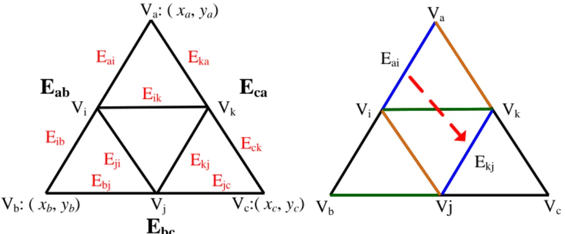
To obtain the same edge function derived, it is improper to use the coordinate of the vertex Vc and Vd for the calculation in Fig. 2.3 (a). Therefore, an edge function recovery scheme is applied to correct edge function calculation. The proposed scheme takes the advantage of linear property of line equation and computes the edge functions for the generated triangles. In Fig. 2.5 (a), a triangle is subdivided into four triangles. After subdivision, the edge functions of the small triangles can be computed in the following steps.

Step 1: Compute the edge functions: Eab, Ebc, and Eca of the original triangle using Eqs. (2.6), (2.7) and (2.8).

Step 2: Compute the constant difference values: ∆Cab, ∆Cbc and ∆Cca in Eqs. (2.9), (2.10), and (2.11). The slopes of the three edge functions are expressed in the following.

) ( 2 1 )) )( ( ) )( (( 2 1 bc ab bc ab b a b c a b b c ab B A A B x x y y y y x x C          (2.9) ) ( 2 1 )) )( ( ) )( (( 2 1 bc ab bc ab c b b a b c b a bc B A A B x x y y y y x x C          (2.10) ) ( 2 1 )) )( ( ) )( (( 2 1 ab ca ab ca a c a b c a a b ca B A A B x x y y y y x x C          (2.11)

of small triangles in Fig. 2.5 with the use of the computed original edge functions and the difference values. For example, Ekj can be computed using Eq. (2.12).

Va Vb Vc Vi Vk Vj Eai Ekj Vi Vk Vj Eai Ekj Ebj Eka Eik Eji Ejc Eck Eib

E

ab

E

ca

E

bc Va: ( xa, ya) Vc:( xc, yc) Vb: ( xb, yb)

Fig. 2.5. Illustration of computing the edge functions for small triangles.

0

: _kj  _kj  _kj 

kj A x B y C

E (2.12)

, where Akj  Aab, Bkj Bab, Ckj Cab Cab. The constant term Ckj can be derived

from the constant term Cab of the edge function Eab by adding the difference value ∆Cab in Eq. (2.9). The other edge functions can be computed in the similar behavior. Finally, the small triangles can be rendered with these edge functions. By the proposed method, the derived edge functions on the sharing edge of any adjacent triangles are the same. Therefore, the rasterization anomaly can be eliminated. The rendering results using the proposed edge function recovery scheme are shown in Fig. 2.6 (a), (b), (c), (d).

(a) Teapot (b) Pawn

(c) Venus (b) Couch Fig. 2.6. Rendering results with the proposed edge function recovery scheme.

In Eq. (2.6), evaluating one edge function requires three subtractions and two multiplications. For a subdivided triangle with Ns segments on each edge, there are total

3NS edge functions to be computed and computation requires 3NS(2 muls + 3 subs) = 6NS muls + 9NSsubs = 6NS muls + 9NSadds (subtraction is regarded as addition). The proposed recovery scheme computes each edge function for the subdivided triangle by adding one difference values. Therefore the computation complexity can be reduced to 3(2 muls + 3 adds) + 3(2 muls + 1 add) + (3NS - 3)(1 add) = 12 muls + (3NS + 9) adds. Thus, the edge function recovery scheme implies an efficient method for computing the

edge functions of subdivided triangles.

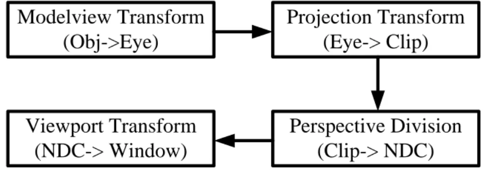
2.3 Dual Space Subdivision Scheme

In the geometry engine, a sequence of transforms is applied to the vertices. A flow chart of the transforms is shown in Fig. 2.7.

Modelview Transform

(Obj->Eye)

Projection Transform

(Eye-> Clip)

Perspective Division

(Clip-> NDC)

Viewport Transform

(NDC-> Window)

Fig. 2.7. Flow chart of the transforms in the geometry engine.

The modelview transform transforms the vertex from object space to eye space by multiplying a 4x4 modelview matrix below.

                                         obj obj obj obj eye eye eye eye w z y x m m m m m m m m m m m m m m m m w z y x 15 14 13 12 11 10 9 8 7 6 5 4 3 2 1 0 (2.13)

In the projection transform, the eye space coordinate is transformed to clip space by multiplying a 4x4 projection matrix below.

                                         eye eye eye eye clip clip clip clip w z y x p p p p p p p p p p p p p p p p w z y x 15 14 13 12 11 10 9 8 7 6 5 4 3 2 1 0 (2.14)

After clipping, the vertices in the clip space will be projected to the projection plane by dividing the w component below. After the perspective division, the

normalized device coordinate (NDC) of each component in the range of [-1, 1] can be expressed in Eq. (2.15).                      clip clip clip clip clip clip NDC NDC NDC w z w y w x z y x / / / (2.15)

Finally, through the viewport transform (viewport mapping), the NDC will be transformed to the window (screen) coordinate.

                           offset NDC scale offset NDC scale offset NDC scale window window window z z z y y y x x x z y x (2.16)

The conventional subdivision-based algorithm subdivides the triangles in the object space or the eye space. As illustrated in Fig. 2.8, the subdivision is performed at the early stage of the pipeline. Because the subdivision generates a large number of vertices, theses vertices bring overhead to the computation and the power consumption to the later stages of pipeline. To reduce the complexity, the dual space subdivision is proposed. ModelView Transform Eye-space coordinate Eye-space normal Perspective Division Viewport Transform Projective Transform Lighting Eye-space coordinate Eye-space normal Eye-space coordinate Eye-space normal Screen-space coordinate Eye-space Subdivision

ModelView Transform Projective Transform Perspective Division Viewport Transform Lighting Screen-space coordinate Eye-space coordinate Eye-space normal Eye-space Subdivision Screen-space Subdivision

Fig. 2.9. Data flow of dual space subdivision.

As illustrated in Fig. 2.9, the subdivision of the proposed scheme is performed after the viewport transform of the pipeline. It subdivides both the coordinates in eye space and window space. The eye space coordinate is required for point-light calculation and the screen space coordinate is used for edge function calculation and other geometry operations. By skipping these transforms including projection transform, perspective division and viewport transform, the computational complexity is remarkably reduced.

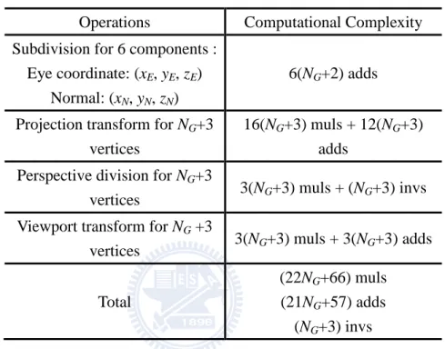
The complexity analysis of the eye space subdivision of a single triangle is given in Table 2.1. The left column lists the operations of subdivision and the corresponding complexity is listed in the right column. NG is defined as the number of the generated intermediate vertices during subdivision. After the triangle is subdivided, there are (NG+3) vertices including the original three vertices. First, the triangle is subdivided in eye space. Each step of the subdivision algorithm involves two vector-additions for eye coordinate (xE, yE, zE) and normal vectors (xN, yN, zN) with total six additions. Therefore, the addition complexity of subdivision is 6(NG+2) additions where two is the number of steps to calculate the difference vectors. After subdivision, all (NG+3) vertices will be transformed by projection transform, perspective division and viewport transform. As described in this subsection, the projection matrix is a 4x4 matrix and the computational complexity of the projection transform is equal to 16(NG+3) muls + 12(NG+3) adds. The perspective division for a vertex requires three multiplications and one inverse and therefore the total computational complexity is 3(NG+3) muls + (NG+3) invs for (NG+3)

vertices. The viewport transform requires three multiplications and three additions for each vertex. The computational complexity is 3(NG+3) muls + 3(NG+3) adds for (NG+3) vertices.

Table 2.1: Complexity analysis of the eye space subdivision

Operations Computational Complexity

Subdivision for 6 components : Eye coordinate: (xE, yE, zE)

Normal: (xN, yN, zN)

6(NG+2) adds

Projection transform for NG+3 vertices

16(NG+3) muls + 12(NG+3) adds

Perspective division for NG+3

vertices 3(NG+3) muls + (NG+3) invs

Viewport transform for NG +3

vertices 3(NG+3) muls + 3(NG+3) adds

Total

(22NG+66) muls (21NG+57) adds

(NG+3) invs

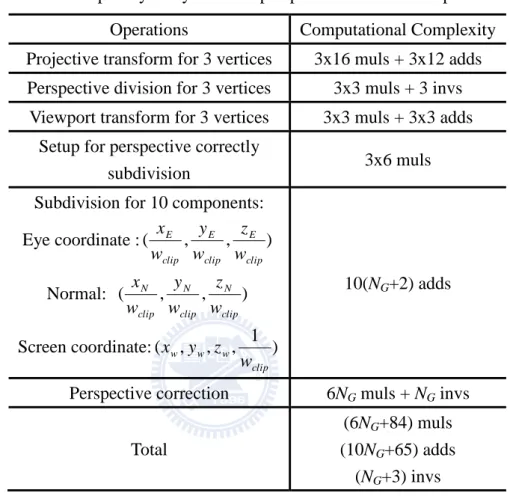
Compared to the eye space subdivision, the dual space subdivision subdivides triangles after the viewport transform. Thus, the projective transform, perspective division and viewport transform are performed for the three vertices. The complexity is listed in Table. 2.2. After the viewport transform, the eye coordinates, normal vector and the window coordinate will be subdivided. To have perspective correct eye coordinates and normal vectors for the intermediate vertices, a setup for perspective correction is performed by dividing the eye coordinates and normal vectors by the wclip term. The computational complexity of the setup is six multiplications for each vertex. After setup, the subdivision is performed for the coordinates in two spaces and the normal vector and the computational complexity is 10(NG+2) additions. The final step is perspective correction which divides the eye coordinates and normal vectors by the 1/wclip term of

intermediate vertices. Since there are NG intermediate vertices and six divisions are required for each perspective correction, the computational complexity is 6NG muls +

NG invs.

Table 2.2: Complexity analysis of the perspective correct dual space subdivision

Operations Computational Complexity

Projective transform for 3 vertices 3x16 muls + 3x12 adds Perspective division for 3 vertices 3x3 muls + 3 invs

Viewport transform for 3 vertices 3x3 muls + 3x3 adds Setup for perspective correctly

subdivision 3x6 muls

Subdivision for 10 components:

Eye coordinate :( , , ) clip E clip E clip E w z w y w x Normal: ( , , ) clip N clip N clip N w z w y w x Screen coordinate:( , , , 1 ) clip w w w w z y x 10(NG+2) adds

Perspective correction 6NG muls + NG invs

Total

(6NG+84) muls (10NG+65) adds

(NG+3) invs

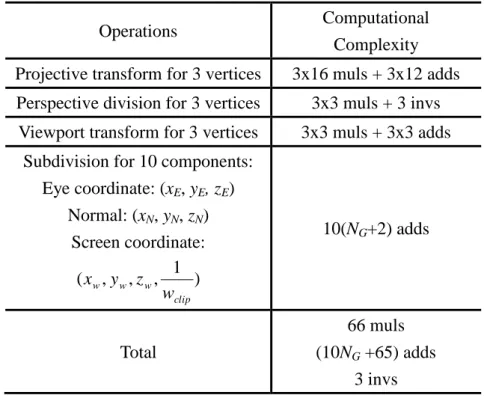
The dual space subdivision is able to provide the perspective correct eye coordinates and normal vectors for light intensity calculation. The computation can be further reduced while the perspective incorrectly subdivision is used and the setup and correction can be skipped. This perspective incorrectness of the intensity on the rendered object can be neglected because human eye is not sensitive to the light intensity of small difference. The complexity of the proposed perspective incorrectly dual space subdivision scheme is listed in Table. 2.3.

Table 2.3: Complexity analysis of the perspective incorrect dual space subdivision

Operations Computational

Complexity Projective transform for 3 vertices 3x16 muls + 3x12 adds

Perspective division for 3 vertices 3x3 muls + 3 invs Viewport transform for 3 vertices 3x3 muls + 3x3 adds

Subdivision for 10 components: Eye coordinate: (xE, yE, zE) Normal: (xN, yN, zN) Screen coordinate: ) 1 , , , ( clip w w w w z y x 10(NG+2) adds Total 66 muls (10NG +65) adds 3 invs

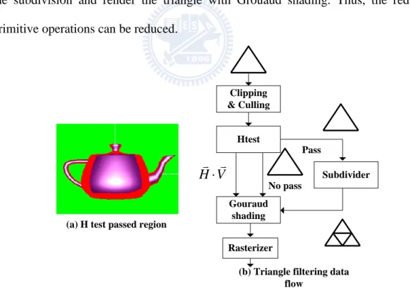
2.4 Triangle Filtering Scheme

To reduce the computation for primitive-level operations, the filtering scheme as shown in Fig. 2.10 is added to the proposed algorithm. The filtering scheme is a hybrid scheme that combines culling/clipping before subdivision and highlight test.

The backface culling in the graphics pipeline is used to test whether a triangle is a backface to the eye direction by the sign of the inner product of the face normal vector and eye direction vector. If a triangle is a backface, it will be discarded and not rendered. In the subdivision algorithm, a triangle will be subdivided into small ones. Performing culling test for these triangles individually brings significant overhead to the computation and power consumption. Because the generated triangles and the original triangle are on the same plane, the face normal vectors are parallel to each other. Therefore, the inner products of these face normal vectors and the eye direction vector will be the same. The statement implies that there is no need to perform backface culling test for each generated triangle since the results will be the same. Hence, in the

proposed algorithm, the subdivision is performed after culling test. If the original triangle is culled, the subdivision is unnecessary. Otherwise, all generated triangles are rendered without culling test. Clipping is another primitive level operation in the pipeline. Since the subdivision is performed after clipping, the generated triangles of the clipped original triangle are guaranteed to be inside the view frustum. Therefore, it is not necessary to re-clip these triangles.

To reduce the redundant subdivision, the subdivision-based algorithm usually includes the highlight test scheme. In the proposed algorithm, the mixed-shading [9][10] for the highlight test is adopted. The scheme tests the HV term of the original three vertices. While one of the H V term is greater than the threshold value, the triangle will be subdivided. If all HV terms are smaller than the threshold value, we bypass the subdivision and render the triangle with Grouaud shading. Thus, the redundant primitive operations can be reduced.

Htest Clipping & Culling Gouraud shading Subdivider Pass Rasterizer (a) H test passed region

(b) Triangle filtering data flow

No pass

V H 

Fig. 2.10. Data flow of the triangle filtering scheme.

2.5 Triangle Setup Variable Sharing Scheme

triangle setup variable sharing scheme is exposed in this section. The concept of the setup reusing result has been shown in [15]; however, the detailed description is not given. During rasterization, the vertex attributes are linearly interpolated for each pixel. These attributes include screen coordinates, texture coordinates, depth values, fog factors, light intensities and etc. The interpolation usually makes the use of the plane equation [17]. An example is given in Fig. 2.11, where (xi, yi) is the window coordinates of the triangle and ui is the attribute to be interpolated. The attribute plane defined by ui is obtained by solving Eq. (2.17).

                    i i i i i i i i i C y B x A u C y B x A u C y B x A u 2 2 2 1 1 1 0 0 0 (2.17)

After solving the plane coefficients Ai, Bi and Ci, the attribute ui for any pixel in the triangle can be obtained by substituting the coordinate into Eq. (2.17). Generally, Eq. (2.17) can be recast in Eq. (2.18) and Eq. (2.19).

           1 1 1 ] [ ] [ _{0 1 2} 2 1 0 2 1 0 y y y x x x C B A u u u _{i i i} (2.18) -1 2 1 0 2 1 0 2 1 0 1 1 1 ] [ ] [            y y y x x x u u u C B Ai i _i (2.19)

In Eq. (2.19), the coefficients [Ai ,Bi, Ci] of any attribute plane can be computed by multiplying a 3x3 inverse matrix, where the inverse matrix is composed of the coordinates [xi, yi, 1] of the triangle. Therefore, once the inverse matrix is available, it

can be used to compute any coefficient for interpolating the attributes of the same triangle. Thus, the cost for setup one attribute is generally a 3x3 matrix multiplication.

The generated triangles of the subdivision algorithm increase the complexity for triangle setup. Because the generated triangles are on the same plane, they define the same attribute plane for each attribute. The coefficients of the attribute planes can be shared by the generated triangles without re-computing these coefficients. As illustrated in Fig. 2.11, the triangle is subdivided into four small triangles and therefore the original setup cost for one vertex attribute of these triangles are four 3x3 matrix inversions and four 3x3 matrix multiplications. With the setup variables sharing scheme, the setup only requires one 3x3 matrix inversion and one 3x3 matrix multiplication because the pre-computed variables are shared by the small triangles. Reusing these coefficients eliminates the subdividing and the setting up vertex attributes for the small triangles. Most rasterization algorithms start rasterization from a pixel with initial attribute values and evaluate the attribute values of next pixel in an incremental manner. It is necessary to compute the initial attribute values for each generated triangles in Eq. (2.20). It takes three multiplications to re-setup for each generated triangle in tile-based traversal scheme [16].                     1 ] [ y x C B A C y B x A u _{i i i i i i} (2.20)

(x0, y0, u0) (x1, y1, u1) (x2, y2, u2) Initial Point 1 Initial Point 2 Initial Point 3 x  y 

Chapter

3

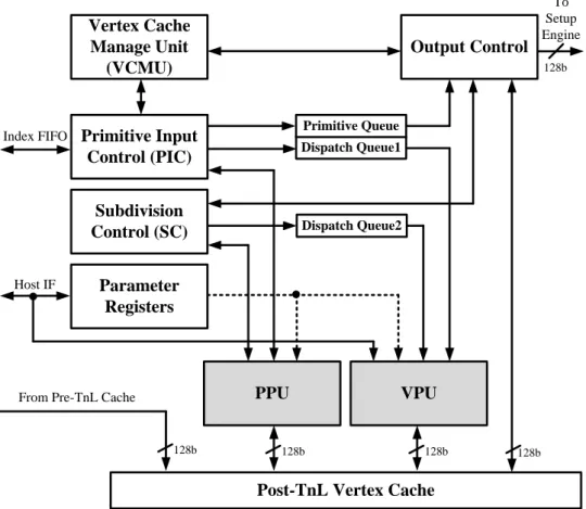
Proposed Geometry Engine Architecture

In this chapter, a power efficient geometry engine (GE) architecture for 3D graphics pipeline architecture is proposed. Several kernel blocks including the primitive input control (PIC), the primitive processing unit (PPU), vertex processing unit (VPU) and vertex cache management unit (VCMU) are proposed to optimize the power consumption and to support the scalable quality mechanism via the proposed subdivision algorithms. The proposed GE supports the scalable quality mechanism via the proposed subdivision algorithm. The users can choose the most efficient configuration for the graphics processing according to the requirements of the shading quality and the power budget. The supported scalable quality levels are level-0, level-1 and level-2. The overall architecture of the proposed GE is depicted in Fig. 3.1 and the detailed descriptions of each block are given in the following subsections.

Post-TnL Vertex Cache Dispatch Queue1 128b 128b 128b To Setup Engine

From Pre-TnL Cache Host IF Index FIFO 128b Primitive Input Control (PIC) Vertex Cache Manage Unit (VCMU) 128b Subdivision Control (SC) Parameter Registers Primitive Queue PPU VPU Output Control Dispatch Queue2

Fig. 3.1. Overall architecture of proposed GE architecture.

3.1 Primitive Input Control (PIC)

The primitive input control (PIC) processes the input primitive information from the host. The PIC reads one index from index FIFO at a time and accesses cache tag to check whether the vertex with the index exists in the vertex cache. Once the cache misses, the PIC requests fetching the vertex data (object coordinate and normal vectors) from the pre-TnL cache. The vertex data returned from the pre-TnL cache will be stored in the post-TnL cache. If the cache hits, the vertex data are not fetched because it is already in the post-TnL cache. The triangles defined by the indices are assembled in PIC and then the backface culling test is issued for the assembled triangles. If the triangle is backface, it will be discarded from PIC. Otherwise, the triangle is pushed to the primitive queue (PQ) and the vertices that belong to the triangle are push the dispatch queue 1 (DQ1) for further processing.

3.2 Primitive Queue (PQ)

The primitive queue (PQ) is a FIFO that buffers the triangles for processing. Each entry of PQ stores the cache entries of three vertices of a triangle. The triangle that passed the culling test is pushed to PQ by PIC. After all vertices of the triangle are transformed and lit, the output control pops the triangle from PQ and read the vertex data (window coordinate and light intensity) of the triangle from vertex cache memory and then output to the setup engine.

3.3 Dispatch Queue (DQ)

The dispatch queue (DQ) is used to keep the vertices under processing. As illustrated in Fig. 3.2, the dispatch queue contains two vertex-cache-entry buffers. The vertex-cache-entry buffer contains the entry addresses of the vertices in the cache. The VPU can access the vertex data with this information. When the vertices in buffer 1 in Fig. 3.2 are processed in VPU, the PIC is able to continue pushing unprocessed vertices into buffer 2 in Fig. 3.2. After all vertices of buffer 1 are processed and buffer 2 is full, the buffers swap. Then, the VPU processes the vertices in buffer 2 and the PIC pushes the unprocessed vertices to buffer 1. With the ping-pong buffer architecture, the PIC and VPU can operate concurrently and thus the performance is increased. In DQ, the size of each buffer is six which is the optimized size for the three-level subdivision algorithm.

V6 V5 V4 V3 V2 V1 V12 V11 V10 V9 V8 V7 5b 5b 5b To VPU 5b 5b From PIC/SC 5b

Vertex cache entry buffer 1

Vertex cache entries buffer 2

3.4 Vertex Cache Management Unit (VCMU)

The vertex cache manage unit (VCMU) is a vertex cache tag unit for the post-TnL vertex cache. The post-TnL cache contains 16-tag entries and each entry has seven fields as illustrated in the first entry in Fig. 3.3. Compare with other works [19], the tag entry contains a reference count field to trace the number of references to the vertex in the tag entry. The primitive processing unit (PPU), VPU, and PIC can operate concurrently. The reference count field is necessary to prevent the data of the vertices which are under processing from being replaced by the incoming vertices. When the PIC requests the VCMU to check whether a vertex exists in the cache, the searched vertex index is compared with the index field of each tag entry. When the index matches one of the valid tag entries, the Entry_hit signal of the tag entry asserts and the VCMU returns hit signal. Since one more vertex enters the pipeline and refers to the data in the cache entry, the value of the reference count field of the tag entry is added by one. The entry address of the vertex is obtained by encoding the hit_vector in Fig. 3.3 and returned to PIC. If the index does not match any tag entry, the VCMU returns miss signal. Before PIC requests fetching the vertex data, the VCMU searches for one free tag entry and allocates it to the vertex. A tag entry is available to be allocated when the valid field is 0 or the reference is 0. When these conditions are met, the Entry_free signal asserts. The allocated entry address for the vertex is obtained by encoding the free_vector in Fig. 3.3 and returned to PIC. In Fig. 3.3, the reference count in the tag entry subtracts by one when a vertex referring to it exits the pipeline. When the cache hits, the in_pipe and lit fields indicate that the vertex is processed in the pipeline and lit, respectively. When one of the two fields is set to 1, the vertex is not pushed into DQ since it is already been transformed and lit. The window coordinate and intensity can be read from the cache directly. The Htest_result field stores the result of the highlight test

for the subdivision algorithm. With this field, the power can be reduced because the highlight test for the stored vertex is only performed once and the result can be reused by the triangles the vertex.

Tag Entry 1

Entry hit_0 Entry free_0 Entry hit_1 Entry free_1

…

…

Tag Entry 15

Entry hit_15 Entry free_15 Entry free_vector Entry hit_vector 16b 16b Index to search 10b Index Zero_ref In_pipe Lit Htest_result

Ref_count

=

0 1 Valid 10b 1b 1b 1b 0 1 0 1

Tag

Entry 0

…

…

Fig. 3.3. Illustration of the vertex cache management unit.

3.5 Primitive Processing Unit (PPU)

The primitive processing unit (PPU) performs primitive-level operations including backface culling and subdivision algorithm. The backface culling is performed in object space [20] to remove the unnecessary transforms for the vertices of the culled triangles. The subdivision algorithm makes the use of the forward difference to subdivide the triangles. These operations are similar such that the datapath architecture can reused for area efficiency. The block diagram of the proposed PPU architecture is depicted in Fig. 3.4, where the bit with of each node has been marked for clear representation. As illustrated in Fig. 3.4, before culling or subdivision starts, the controller loads the data

of the three vertices of the triangle in the cache into the input buffers. The eye position in the object space is stored in the eye position buffer which is set by the host when the eye position is updated. The PPU is able to write the data into the vertex cache because the subdivision algorithm generates intermediate vertices. These vertices are written back to the cache and be read by the VPU for further processing.

Control Unit

To vertex cache read channel

From vertex cache read channel

From primitive input ctrl/ subdivision ctrl

Vertex0 input buffer (128b) Vertex1 input buffer (128b) Vertex2 input buffer (128b) 128b

Datapath

128b 128b 128b

Eye position buffer (96b)

128b

To vertex cache write channel 96b 128b MUL (16bx16b) ADD_SU B(32b) SUB3 (32b) SUB2 (32b) SUB1 (32b) Hdiff (128b) R0 (32b)

Intermediate value registers Vdiff (128b)

Vtmp (128b)

Htmp (128b) R1 (32b)

Fig. 3.4. Block diagram of the primitive processing unit.

3.6 Vertex Processing Unit (VPU)

The vertex processing unit (VPU) performs vertex-level operations including vertex transformation and lighting operation. The operations covers modelview transform, projection transform, perspective division, normal transform, viewport transform, vector normalization and Blinn-Phong reflection model. The Blinn-Phong

reflection model [4] can be formulated in Eq. (3.1). s n d a N L I N H I I I  ( ) (  ) (3.1) Where Ia, Id, Is,N 

,L,H denote the ambient intensity, diffuse intensity, specular intensity, normalized normal vector, normalized light vector, and normalized halfway vector, respectively. The halfway vector

2 V L H    _

 is the vector between the light direction vector L and the viewing vector V. In Fig. 3.1, so as to maximize the performance, the VPU is designed to process a batch of vertices in DQ at the same time. The block diagram of VPU architecture is depicted in Fig. 3.5, where the bit width of each node has been marked for clear representation. The vertex data are read from the read channel of the vertex cache. Then, they are transformed and lit in the reconfigure datapath (RDP). The register file stores the intermediate values for the vertices under processing. The constant memory stores the matrix parameters and the light parameters for transforms and lighting, respectively. The content of the constant memory is set by the host before the GE starts. Finally, the vertices are read from the register file and written back to vertex cache when all vertices in the batch are transformed and lit.

Control Unit

To vertex cache read

channel Constant Memory (16x128) Register file (48x128) Reconfigurable Datapath From vertex cache read

channel

Output data buffer

32b 32b 32b 32b Configuratio n Rom (6x90) 92b 128b 128b 128b 128b 128b

To vertex cache write channel To vertex cache write

channel

128b From dispatch queue

PE1 PE2

PE3 SFU

FIFO

Write back path

Fig. 3.5. Block diagram of the vertex processing unit.

Considering the trade-off for the power, area and vertex processing performance of the GE architecture, the operations listed in Chapter 3 are disassembled into the simpler atomic operations. For example, the modelview transform involves a 4x4 matrix multiplication which can be achieved by four dot product operations. The un-disassembled operations and the atomic operations define the minimum set of operations supported by the RDP. The RDP can be configured to different modes to achieve these operations. These configuration modes are summarized in Table 3.1. The RDP is a pipelined SIMD datapath architecture for high performance vertex processing. The RDP is composed of three processing elements (PEs), one special function unit (SFU) and one FIFO as shown in Fig. 3.5. By reconfiguring three PEs, the SFU and the interconnection between these PEs, the RDP can realize all the transform and lighting operations listed in Table 3.1. For a complicated operation such as the vector

normalization, the RDP is configured to be an efficient pipelined datapath. By processing a batch of vertices at the same time and filling the pipeline, the average cycle for the operation is reduced compared with other architectures that process one vertex one at one time. The detailed descriptions about the RDP are given in the following subsections.

Table 3.1: Configuration modes for RDP Configuration

Mode Function Description

trans_dp Dot product for transform light_dp Dot product for lighting

vec_norm Vector normalization

Pd Perspective division

Pow Powering

vec_sub Vector subtraction

3.6.1 Processing Element (PE)

The architecture of the processing element (PE) is illustrated in Fig. 3.6, where the PE is a three-stage pipeline. At the first stage, the 32-bit fixed-width Booth multiplier multiplies two numbers and generates two partial products. The 32-bit fixed-width Booth-based squarer [21] is used to perform squaring operation. A dedicated squarer consumes less power dissipation than that of a general-purpose multiplier. The outputs of the squarer are two partial products. At the second stage, the 32-bit 4-2 compressor is used to add four inputs and generates two partial products. Finally, at the last stage, the adder-subtractor unit adds or subtracts two numbers and produces the final output. The function of the adder-subtractor is controlled by the MODE signal in Fig. 3.6. The multiplexers in PE control the data flow for different operations. The PE can be

multiplication-accumulation (MAC), addition (ADD) and subtraction (SUB) as shown in Figs. 3.7, 3.8, 3.9, and 3.10, respectively.

The datapath of multiplication (MUL) operation is illustrated in Fig. 3.7 and marked with dashed lines. The first stage of MUL generates the partial products by multiplying two numbers of the input registers REG_B and REG_C. The partial product outputs are registered in the pipeline registers REG_F and REG_G and then are summed up in the adder-subtractor unit. The datapath of square (SQR) operation is illustrated in Fig. 3.8. The squarer squares the number in the input register REG_D and generates two partial products. The partial products are registered in the pipeline register REG_H and REG_I and then are summed up in the adder-subtractor unit. The datapath of the multiplication-accumulation (MAC) operation is illustrated in Fig. 3.9. For the MAC operation, the number in the input register REG_B is multiplied by the number in the input register REG_C and the result is added to the number in the input register REG_A to produce a result of MAC. At the first stage, the numbers in REG_B and REG_C are multiplied and the partial products are registered in the pipeline register REG_F and REG_G. The number in the register REG_A is directly passed to the pipeline register REG_E. At the second stage, the partial products in REG_F and REG_G and the number in REG_E are added with the 4-2 compressor and the resulting partial products are registered in the REG_J and REG_K. At the last stage, the partial products in register REG_J and REG_K are summed up in the adder-subtractor unit to produce the result. The datapath of addition (ADD) and subtraction (SUB) operations are illustrated in Fig. 3.10. The pipeline registers REG_J and REG_K are configured to be the input registers for the ADD and SUB operations. The numbers in REG_J and REG_K are added or subtracted according to the target operations.

32x32 Fixed-width

Booth multiplier Fixed-width sqrarer REG_H REG_G REG_I REG_F REG_D REG_C REG_B REG_A REG_E 4-2 compressor 0 0 In. E port In. F port In. G port In. H port REG_K REG_J In. I port In. J port Add-Sub In. MODE In. D port In. C port In. B port In. A port Out. A port Out. B port Out. C port Out. D port Out. E port Out. F port 32b 32b 32b 32b 32b 32b 32b 32b 32b 32b 32b 32b 32b 32b 1b 32b 32b 32b 32b 32b 32b 32b 32b 32b 32b Mux Mux Mux Mux

Mux Mux Mux Mux

M u x M u x

32x32 Fixed-width

Booth multiplier Fixed-width sqrarer REG_H REG_G REG_I REG_F REG_D REG_C REG_B REG_A REG_E 4-2 compressor 0 0 In. E port In. F port In. G port In. H port REG_K REG_J In. I port In. J port Add_Sub In. MODE In. D port In. C port In. B port In. A port Out. A port Out. B port Out. C port Out. D port Out. E port Out. F port 32b 32b 32b 32b 32b 32b 32b 32b 32b 32b 32b 32b 32b 32b 1b 32b 32b 32b 32b 32b 32b 32b 32b 32b 32b Mux Mux M u x M u x

32x32 Fixed-width

Booth multiplier Fixed-width sqrarer REG_H REG_G REG_I REG_F REG_D REG_C REG_B REG_A REG_E 4-2 compressor 0 0 In. E port In. F port In. G port In. H port REG_K REG_J In. I port In. J port Add_Sub In. MODE In. D port In. C port In. B port In. A port Out. A port Out. B port Out. C port Out. D port Out. E port Out. F port 32b 32b 32b 32b 32b 32b 32b 32b 32b 32b 32b 32b 32b 32b 1b 32b 32b 32b 32b 32b 32b 32b 32b 32b 32b M u x M u x

32x32 Fixed-width

Booth multiplier Fixed-width sqrarer REG_H REG_G REG_I REG_F REG_D REG_C REG_B REG_A REG_E 4-2 compressor 0 0 In. E port In. F port In. G port In. H port REG_K REG_J In. I port In. J port Add_Sub In. MODE In. D port In. C port In. B port In. A port Out. A port Out. B port Out. C port Out. D port Out. E port Out. F port 32b 32b 32b 32b 32b 32b 32b 32b 32b 32b 32b 32b 32b 32b 1b 32b 32b 32b 32b 32b 32b 32b 32b 32b 32b M u x M u x

32x32 Fixed-width

Booth multiplier Fixed-width sqrarer REG_H REG_G REG_I REG_F REG_D REG_C REG_B REG_A REG_E 4-2 compressor 0 0 In. E port In. F port In. G port In. H port REG_K REG_J In. I port In. J port Add_Sub In. MODE In. D port In. C port In. B port In. A port Out. A port Out. B port Out. C port Out. D port Out. E port Out. F port 32b 32b 32b 32b 32b 32b 32b 32b 32b 32b 32b 32b 32b 32b 1b 32b 32b 32b 32b 32b 32b 32b 32b 32b 32b Mux Mux M u x M u x

Fig. 3.10. Illustration of addition/subtraction operation.

3.6.2 Special Function Unit (SFU)

The special function unit (SFU) provides various arithmetic operations including the inverse (INV), inverse-square-root (InvSqrt) and power (POW) operations. These operations are used for vertex processing. To achieve low-power arithmetic operations, the SFU adopts the logarithmic number system (LNS) [22-24] where the complicated arithmetic operations are replaced by the simple arithmetic.

The architecture of SFU is depicted in Fig. 3.11, where the bit width of each node has been marked for clear representation. For the INV and the InvSqrt operations, the

logarithmic convertor as shown in the top gray region of Fig. 3.11 converts the input number m to its logarithmic number M. Then, the number M is inversed through the Inv block to produce the result ~M. In the shift block, the number ~M is shifted right one bit to obtain (~M)>>1 for InvSqrt operation or directly bypassed for Inv operation. The behavior of the shift block controlled by the Config[1] port. The output logarithmic number (~M)>>1 or ~M of the shift block is then converted to their ordinary fixed-point number m 1 or m 1

by the antilogarithmic convertor as shown in the bottom gray

region of Fig. 3.11.

For the POW operation n

m , the number m is converted to its logarithmic number

M. To compute nM, the multiplier is required for multiplication. However, the real multiplier is not included in SFU to achieve area and power-efficient feature. Because the processing element (PE) in the RDP shown in Fig. 3.6 can be configured to be a multiplier to compute nM. In Fig. 3.11, the logarithmic number M is outputted to a PE which is configured as a multiplier and multiplies to the number n. The result nMis then returned from the PE and converted to its ordinary number n

m . The Config[2] controls the source for the antilogarithmic convertor.

3.6.3 FIFO

As mentioned above, the RDP constructs an efficient pipeline datapath for complicated operations. In some configuration modes, some of the input data are used in the later stage of the pipeline. However, bypassing these data with pipeline registers stage by stage is not efficient for power consumption. To avoid the unnecessary data transfers between the pipeline registers, the FIFO is included in the RDP.

Input Register Normalize neg sign Log Converter Pipeline Register Shift Pipeline Register Antilog Converter Pipeline Register Underflow Detection Output register neg Ash 32b 31b 31b exp norm 5b 16b neg 1b 1b 5b 16b 16b 16b 16b 17b 17b 17b 32b 32b 5b 5b 5b neg Config[2] Config[1] Config[0] To multiplier From multiplier 5b 16b Output Register Inv 1b Mux

Fig. 3.11. Block diagram of the special function unit.

3.6.4 Interconnection of Configuration Modes

In this section, the interconnections between the building blocks for different configuration modes are described. For clearly explanation, the block diagram of the processing element (PE) is simplified. The geometry transforms in Eq. (2.13) and Eq. (2.14) multiply a 4x4 matrix by a 4x1 column vector. The matrix-vector multiplication

can be replaced by four 4-component inner product operations. In Eq. (3.2), the 4-component inner product calculation employs four multiplications and therefore requires four multipliers.





_{1 2 1 2 1 2 1 2} 2 2 2 2 1 1 1 1 x x y y z z w w w z y x w z y x                     (3.2)

Because the term wobj in the column vector in Eq. (2.14) is always one and the projection matrix in Eq. (2.15) is a sparse matrix, these transforms can be achieved by the 3-component inner products and the additions as expressed in Eq. (3.3). The datapath for the operation in Eq. (3.3) is composed of three processing elements (PE) and the interconnections between PEs are illustrated in Fig. 3.12. At the first stage, the three multiplications are performed using the partial-product multiplier in the PEs, respectively. The addend w is directly passed to the next stage. At the second stage, the partial products and the addend w are compressed by the 4-2 compressor. Finally, the resulting partial products are summed up in the adder-subtractor unit of the central PE to produce the result.





1 2 1 2 1 2 1 2 2 2 1 1 1 1 1 w z z y y x x z y x w z y x                    (3.3)