減少H.264/AVC的框間模式選取中所使用的測試次數並以多執行緒加速運算

國

立

交

通

大

學

資訊科學與工程研究所

碩

士

論

文

減少 H.264/AVC 的框間模式選取中所使用

的 測 試 次 數 並 以 多 執 行 緒 加 速 運 算

Reducing the number of used tested modes in inter mode

decision for H.264/AVC and accelerating with

multithreading

研 究 生：葉柏宏

指導教授：林正中 教授

減少 H.264/AVC 的框間模式選取中所使用的測試次數並以多執行緒 加速運算

Reducing the number of used tested modes in inter mode decision for H.264/AVC and accelerating with multithreading

研 究 生：葉柏宏 Student：Po-Hung Yeh 指導教授：林正中 Advisor：Cheng-Chung Lin 國 立 交 通 大 學 資 訊 科 學 與 工 程 研 究 所 碩 士 論 文 A Thesis

Submitted to Institute of Computer Science and Engineering College of Computer Science

National Chiao Tung University in partial Fulfillment of the Requirements

for the Degree of Master

減少 H.264/AVC 的框間模式選取中所使用的測試次數並以多執行緒 加速運算 學生：葉柏宏 指導教授：林正中 博士 國立交通大學資訊科學與工程研究所 碩士班

摘 要

模式選取在 H.264 的編碼程序中由於它的時間複雜度是一個瓶 頸。在本文中，我們提出了一種新的方法來將框間模式選取的測試 次數由原來的七次降為三次。詳細地，我們辨認最小的兩個框間模 式的輕量成本，並檢查它們的相鄰與否，來決定保留或捨棄一些模 式。我們還平行化一部分的程式碼來加快執行時間。實驗結果證明， 無論何種視訊類型的情況，所提出的方法在執行時間方面改進了效 能，並仍保持幾乎相同的視訊品質與幾乎沒有改變的編碼視訊大小。 關鍵字：模式選取，框間模式，H.264，成本，提前終止，山谷 [葉柏宏君於碩士論文口試通過後，由於健康因素無法於短期內完成 其論文之結構修正，僅能以此論文初稿形式作結] -林正中

Reducing the number of used tested modes in inter mode decision and accelerating with multithreading

Student: Po-Hung Yeh Advisor: Dr. Cheng-Chung Lin

Institute of Computer Science and Engineering National Chiao-Tung University

ABSTRACT

Mode decision at the encoder processing of H.264 is a bottleneck due to its time complexity. In this paper, we propose a new method to reduce the original 7 inter modes to 3. In particular, we identify the smallest 2 light-weight costs of inter modes, and check if they are neighbors or not, to determine whether to save or discard some of the modes. We also parallelize a part of the code to speed up the executing time. The experimental results demonstrate that the proposed methods improve the performance in terms of executing time, regardless of the video types in consideration, and still keep almost the same video quality with almost no change in encoded video size.

誌 謝

首先我要感謝老師的指導提點、學長的幫助，和同學們之間的討 論，讓這篇論文能順利完成，在此致上最誠摯的謝意。 我要特別感謝鍾崇斌教授的指導和翁綜禧學長的協助，他們針對 我以往未曾注意到的弱點提出建言，這正是過去的我所欠缺、未曾 經歷的。以前的我只會精益求精，追逐成功，但他們讓我學習如何 面對失敗挫折克服自身的缺點，度過困難，待人處世，如何看待問 題，讓我更加強韌、茁壯、成熟。 感謝這一路走來曾經鼓勵我、幫助我的人，因為有你們才有現在 的我。 最後謝謝我的父母、姊姊的支持和陪伴，讓我前行。 僅以此篇獻給你們！

Table of Contents

摘 要 ... i ABSTRACT ... ii 誌 謝 ... iii Table of Contents ... iv List of Figures ... v List of Tables ... vi Chapter 1. Introduction ... 1 1.1 Background ... 4 1.2 Related Work ... 7

1.3 Observation and Objective ... 9

Chapter 2. Background ………..11

Chapter 3. The proposed method - Two valleys approximation approach ...11

List of Figures

Figure 1 : Inter coding with 5 reference frames. ... 6 Figure 2 : The valley of early termination. ...10 Figure 3 : Reference [5] performs the 1st reference frame ME to select

the ideal mode. ...12 Figure 4 : RD curves for “Claire” (QCIF). ...21 Figure 5 : RD curves for “Stefan (CIF)”. ...21

List of Tables

Table 1 : Experimental Results for QP=28. ...18

Table 2 : Comparisons with Zhan’s method in [7] when QP=28. ...18

Table 3 : Comparisons with Ma’s method in [8] when QP=28...19

Table 4 : Results for “Claire” (QCIF). ...20

Chapter 1. Introduction

1.1 Overview of H.264

H.264/MPEG-4 AVC [1][2] is a standard for video compression developed by the ITU-T Video Coding Experts Group (VCEG) together with the ISO/IEC Moving Picture Experts Group (MPEG). The encoding schemes of H.264 have 2 types, which are intra and inter coding based on spatial and temporal characteristics, respectively.

The is shown in Figure 1-1 [3].

Figure 1-1: The encoder block diagram of H.264 [3].

Intra-prediction

The earlier video coding standards such as MPEG-4 and H.263 [,] perform motion estimation between only one previous picture and the current picture for the P-picture encoding, that is, only recently previous I- or P-picture is used as a reference picture. The drawback is if a part of the subject picture is lost due to channel error or packet loss,…. To the H.263 v. 2 (H.263+) Annex N, in order to suppress temporal error propagation, it started to provide reference picture selection mode. H.263++ for both error resilience and coding efficiency. and be adopted in H.264. In the H.264/AVC standard, in order to improve coding

efficiency, it provides various block sizes and multiple reference frame based motion estimation.

MB reconstruction

Figure 1-2 shows the run-time percentage of several major function modules in the H.264 encoder [4]. As can be seen from Fig. 1-2, motion prediction and mode decision take the largest portion of computational complexity. Hence, in order to reduce the complexity of H.264 encoder, it is worth to develop the fast inter mode decision.

1.2 Issue

1.3 Motivation

Some studies [3]-[5] focus on exploiting the parallel opportunities for intra mode decision. However, there are a few studies to discuss

about inter mode decision level in parallel. We will try to seek the level(s) in inter mode decision hierarchy which can be executed in parallel.

Chapter 2. Background

2.1 Mode decision scheme in H.264

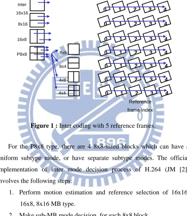
A 16x16-pixel luminance MB (macroblock) to be encoded has 7 inter prediction modes distinguished by different block sizes, including MB partitions of sizes 16x16, 16x8, 8x16, and P8x8, where P8x8 can be sub-divided into sub-MB partitions of sizes 8x8, 8x4, 4x8, and 4x4, as shown in Fig. 1. There is also a 16x16 SKIP mode, which is reserved for two MBs that have no residual. For each valid mode, inter prediction involves two steps, including motion estimation (ME) and reference frame selection. More specifically, inter prediction performs motion estimation for every ref. frame, searches the best predictive block in a search window, and then selects the best ref. frame, as illustrated in Fig.1.

In the selection of the best predictive block, H.264 adopts the RDO (rate-distortion optimized) criterion as the performance index (which is referred as RD cost):

smaller RD value is, the better the performance of video compression becomes.

The cost used by motion estimation is named MCOST shown next:

 J_MotionSAD(s,c)_MotionR



mv



,  

where SAD( cs, ) is the sum of absolute differences between each pixel in the original block s and the predictive block c . mv is the motion vector difference between predicted mv and actual mv. R



mv



is the number of bits representing mv via table lookup. It is a light-weight cost, which means it is a predictive value, not the real reconstructed value.

When RDO option is enabled, mode decision will adopt the mode cost called the RDOcost shown next:

 J_ModeSSD



s,c,Mode|QP



_ModeR



s,c,Mode|QP



,  

where R



s,c,Mode|QP



denotes the bit number for coding this block associated with choosing Mode , SSD is the sum of squared difference

between the original block s and the reconstructed block c , and  is the Lagrange multiplier, QP is the macroblock quantization parameter.

Figure 1 : Inter coding with 5 reference frames.

For the P8x8 type, there are 4 8x8-sized blocks which can have a uniform subtype mode, or have separate subtype modes. The official implementation of inter mode decision process of H.264 (JM [2]) involves the following steps:

8x8 16x8 8x16 Inter 16x16 8x4 4x8 4x4 0 1 2 3 4 0 1 2 3 4 0 1 2 3 4 0 1 2 3 4 0 1 2 3 4 0 1 2 3 4 0 1 2 3 4 Reference frame index P8x8

When RDO option is enabled, for candidate blocks of each mode, the stage of reconstructing the block and computing RDOcost is time consuming. To speed up the computation, a number of techniques under the name of fast inter mode decision (as opposed to exhaustive mode decision) try to exclude some unlikely modes depending on spatial and temporal characteristics, leading to suboptimal result.

2.2 Related Work Brief Review

Exhaustive inter mode decision requires a lot of time to perform ME and compute RDOcost for each mode. Hence many studies focus on reducing the number of modes to be checked.

One of the approaches to reduce computation is the use of early termination [3]-[4]. The algorithm first performs ME and reference frame selection, and then computes RDOcost for a set of modes (16x16 8x8 4x4) to check the characteristics of the cost curve. If it is monotonically decreasing



J_Mode



1616



J_Mode



88



J_Mode



44





, which implies that the encoded MB has the tendency to use larger block sizes, the algorithm will examine the larger blocks, namely, 16x8 or 8x16 modes to obtain the minimizing one and then terminate. On the other hand, if the cost curve is monotonically increasing















J_Mode1616 J_Mode 88 J_Mode 44



, the algorithm will examine the smaller blocks, namely, 8x4 or 4x8 modes to obtain the minimizing

one and then terminate. If the cost curve does not meet any of the monotonic criteria, all other modes must be tested.

Inter coding has multiple reference frames (MREF), and performs ME for every ref. frame before computing mode cost. Many studies focus on analyzing the statistical characteristics of MREF. An observation is that the best selected reference frame is often the nearest one to the current frame [5]. In [5], the algorithm uses MCOST predicted in the 1st reference frame to select the mode with the minimum cost. In [6], fast multi-reference frames motion estimation (MRFME) not only selects the minimizing mode after the 1st reference frame prediction, but also uses a threshold to determine a potential set of modes for further exploration.

Some researchers exploit the spatial and temporal correlations of MBs in adjacent frames to determine the candidate lists. Zhan et al. [7] obtain the current MB (x,y) on the current frame and seek the co-located MB on the previously encoded reference frame, in order to find the best modes of the co-located MB and its surrounding MBs to adjust the candidate list. Ma et al. [8] use neighboring MBs of current or previous frame and motion history to tune the probability of the modes, which is

modes, such that the same amount of tasks can be dispatched to each thread at a time. Accordingly, this study does not use the dynamic reduction mechanism.

2.3 Observation and Objective

We can view the monotonic criterion of early termination [3] [4] from a different perspective. Once the monotonic criterion is met, the cost curve exhibits a single valley, as shown in Fig. 2. Once the valley is identified, we can compute the RDOcosts at the neighboring two points around the valley, and then find the minimum RDOcost among these three points. As illustrated in Fig. 2, the points are clustered at 1 valley (either A1 at 16x16, or A2 at 16x8/8x16) no matter the final results of



168



Mode

J and J_Mode



816



is smaller than J_Mode



1616



or not. In other words, our computation is just based on the valley and its two nearest neighbors. 16x16 16x8 8x16 8x8 8x4 4x8 4x4 16x16 16x8 8x16 8x4 4x8 4x4 8x8 Mode type J( R D O c o st ) A1 A2

Figure 2 : The valley of early termination.

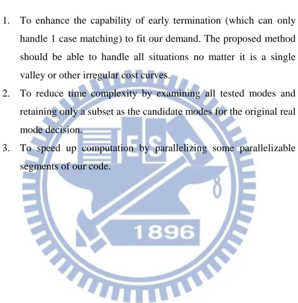
The aims of this study are three-fold:

1. To enhance the capability of early termination (which can only handle 1 case matching) to fit our demand. The proposed method should be able to handle all situations no matter it is a single valley or other irregular cost curves.

2. To reduce time complexity by examining all tested modes and retaining only a subset as the candidate modes for the original real mode decision.

3. To speed up computation by parallelizing some parallelizable segments of our code.

Chapter 3. The proposed method - Two valleys approximation

approach

RDOcost will obtain better Rate-Distortion Optimized compression

quality (including video quality and encoding video sizes), but is computationally expensive. When enable one mode, motion estimation, reference frame selection, reconstruct MB need be performed before computing RDOcost .

MCOST used by motion estimation on each reference frame is a

low-complexity cost than RDOcost . Reference [5] observes the optimal motion vectors are often determined by the nearest reference frame to the current frame. Which means the smallest MCOST of one mode belongs to the first reference frame than others is very often. In [5], the algorithm performs the 1st reference frame ME to select the mode with the best

MCOST , as illustrated in Fig. 3. The research [5] provides an approach

with a light-weight cost to predict the possible modes. Although it can use a fast approach to predict some possible modes, the compression quality is not like the result of using RDOcost . Why not using MCOST to predict RDOcost , just retaining a subset of modes to compute real

RDOcost . This method can collect the costs of all 7 modes and draw the

Figure 3 : Reference [5] performs the 1st reference frame ME to select the ideal mode.

In the previous section, chapter 1.3, we have discussed the monotonic criterion of early termination [3] [4], if one valley is formed, the mode with the smallest cost and its neighboring mode will be tested. The cost curve of early termination is “before completion”. We know the mode with the smallest RDOcost will produce the optimal compression quality. However, whenever testing one mode using RDOcost , it needs to spend a lot of time. The process of early termination is as follows, (and shown in Fig. 2,) in the first phase, the algorithm only tests 3 modes

8x8 16x8 8x16 Inter 16x16 8x4 4x8 4x4 0 0 0 1 2 3 4 0 0 0 0 MCOST P8x8

We have a tool to collect complete 7 modes’ light-weight cost curve, and have a model view to know how to obtain a suboptimal result in a limited number of tested modes. The MCOST (obtained from the 1st reference frame prediction [5]) can predict RDOcost . The half-complete cost curve (inspired by early termination [3] [4]) will process one valley form, to retain the mode with the current smallest cost and its two neighboring modes. We can use the essence to the complete light-weight cost curve.

We will propose our method: Two valleys approximation approach

After the 1st reference frame ME [5], we have MCOST of 7 modes. The cost curve only needs 5 points, so we let the rectangle modes to retain the better one. The remaining 5 modes are 16x16, min(16x8, 8x16), 8x8, min(8x4, 4x8), 4x4, denoted as N1, N2, N3, N4, N5. We just identify the smallest 2 light-weight costs of the 5 modes. If they are neighboring, just retaining the mode with the smallest cost and its 2 neighbors. If they are separated, retaining the 2 modes, adding the lowering valley’s one neighbor as the third candidate. Limit these 3 modes to compute RDOcost , not to expand too many candidate modes that the consumption of the computation time.

The pseudo code is described as follows:

modes.

2. Reduce from 7 to 5 modes, denoted as a set N with elements 5 1 ~ N N , as follows:



16 16



1JMCOST  N ,











16 8, 8 16



min 2  JMCOST  JMCOST  N ,



8 8



3 JMCOST  N ,











8 4 , 4 8



min 4  JMCOST  JMCOST  N ,



4 4



5 JMCOST  N .

3. Reduce from 5 to 3 modes, denoted as a set C. Compute the top-2 minima of J_MCOST

 

N_i , with i1~5. Denote the mode with the smallest MCOST as N_min1 and the bigger one as N_min2.

4. Let d  min1min2 , if d 1, namely N_min1 and N_min2 are adjacent, go to step5; otherwise, go to step6.

5. Let CN_min1, and N_min1’s 2 neighbors, go to step7.

6. Let CN_min1, N_min2, N_min1’s neighbor, which has smaller MCOST go to step7.

7. Use SKIP mode and the 3 modes in C for real mode decision, and choose the best mode from the union of C and SKIP mode.

2

N (min(16x8, 8x16)) modes by 2 threads, if these two modes are both

in C. Note that the 4 8x8 sub-MBs of the P8x8 mode use the same subtype in the steps 1-6, and use separated subtype modes in step 7.

The task of each thread is independent, and the workloads dispatched to each thread are more or less equal in our design. As how to distribute the threads to map the available computing units, this is determined by the scheduling policy of the library of parallel language or the implement design for a cluster. Here we use the parallel language library that support load balance [9] to be used in our method.

Chapter 4. Experimental results

4.1 Introduction

The proposed algorithm was implemented based on H.264 reference encoder JM 16.2 [2] which uses 7-mode decision. The encoder with 5 reference frames adopts the following settings: full search, search range

32

 , CABAC entropy coding method, and quantization parameter (QP) = 28, 32, 36, 40. The simulation environment is based on Pentium Dual 2.0 GHz, 2 GB DDR2, Fedora 9 Linux kernel 2.6.25, gcc 4.3.0 compiler with OpenMP 2.5 library.

The tested sequences for our experiments are QCIF format: Carphone, Claire, Coasguard; CIF format: Coasguard, Container, Mobile, News, Satefan. The structure of encoded frames is IPPP, in which each sequence will be encoded to the first frame, I frame, and 99 P frames that disable intra modes for inter slices. The frame rate is 30 per second.

Our experiments are based on 3 different conditions, including original 7-mode decision (Original), the proposed algorithm (Proposed),

of different values of QP on the same video sequence, where the results are shown via RD curves.

4.2 Experiment 1.

In this experiment, we use all video sequences with QP=28, to evaluate 3 performance metrics, including time reduction



Time



, PSNR gain



PSNR



, and bitrate reduction



Bitrate



, as defined next:

    100% original original proposed Time Time Time Time     PSNRPSNR_proposedPSNR_original       100% original original proposed Bitrate Bitrate Bitrate Bitrate  

PSNR is the peak signal to noise ratio, which reflects the encoded video quality. A higher value of PSNR indicates the less distortion. In our experiment, we only adopt luminance Y-PSNR, which is the most

important part of PSNR. Bitrate is the bit number needed to encode a video sequence.

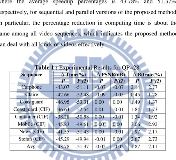
The results for all selected video sequences are shown in Table 1, where the average speedup percentages is 43.78% and 51.37%, respectively, for sequential and parallel versions of the proposed method. In particular, the percentage reduction in computing time is about the same among all video sequences, which indicates the proposed method can deal with all kinds of videos effectively.

Table 1 : Experimental Results for QP=28.

Sequence Time(%) PSNR(dB) Bitrate(%)

P P(t2) P P(t2) P P(t2) Carphone -43.07 -51.11 -0.07 -0.07 2.14 2.77 Claire -42.66 -52.48 -0.09 -0.05 0.45 1.28 Coastguard -46.95 -53.31 0.00 0.00 1.49 1.37 Coastguard (CIF) -46.64 -52.54 0.01 -0.01 1.84 1.73 Container (CIF) -38.28 -50.58 0.00 -0.01 1.34 1.92 Mobile (CIF) -45.83 -49.61 0.00 0.00 3.06 2.92 News (CIF) -41.55 -51.43 0.00 -0.01 1.97 2.17 Stefan (CIF) -45.29 -49.94 -0.01 0.00 2.67 2.73 Avg. -43.78 -51.37 -0.02 -0.02 1.87 2.11

Claire [7] -70.21 -0.09 1.11 Proposed _{-42.66 -0.09 0.45} P (t2) _{-52.48 -0.05 1.28} Coastguard [7] -30.64 -0.01 0.14 Proposed _{-46.95 0.00 1.49} P (t2) _{-53.31 0.00 1.37} Container (CIF) [7] -63.24 -0.04 0.54 Proposed _{-38.28 0.00 1.34} P (t2) _{-50.58 -0.01 1.92} Stefan (CIF) [7] -22.89 -0.02 0.14 Proposed _{-45.29 -0.01 2.67} P (t2) _{-49.94 0.00 2.73}

Table 3 : Comparisons with Ma’s method in [8] when QP=28.

Sequence Method Time

(%) PSNR (dB) Bitrate (%) Coastguard (CIF) [8] -51.74 -0.04 1.64 Proposed _{-46.64 0.01 1.84} P (t2) _{-52.54 -0.01 1.73} Container (CIF) [8] -61.43 -0.06 4.89 Proposed _{-38.28 0.00 1.34} P (t2) _{-50.58 -0.01 1.92} Mobile (CIF) [8] -45.97 -0.05 3.43 Proposed _{-45.83 0.00 3.06} P (t2) _{-49.61 0.00 2.92} Stefan (CIF) [8] -55.90 -0.05 4.39 Proposed _{-45.29 -0.01 2.67} P (t2) _{-49.94 0.00 2.73}

Zhan’s method [7] is faster on the sequences with large static areas (Claire, Container), but the proposed method (especially the parallel version) reduces the execution time evenly. In comparison with Ma’s method [8], for the sequence with low-speed motion (Container), the

proposed method (t2) is slower than theirs, but with a better bitrate. For the other sequences, there are no big differences in performance.

4.3 Experiment 2.

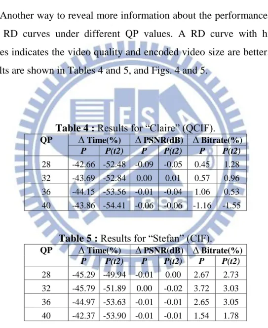
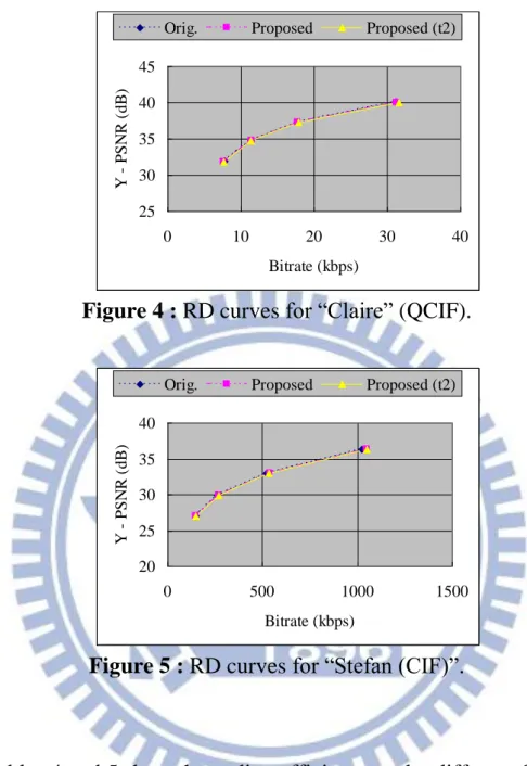
Another way to reveal more information about the performance is to plot RD curves under different QP values. A RD curve with higher values indicates the video quality and encoded video size are better. The results are shown in Tables 4 and 5, and Figs. 4 and 5.

Table 4 : Results for “Claire” (QCIF).

QP Time(%) PSNR(dB) Bitrate(%) P P(t2) P P(t2) P P(t2) 28 -42.66 -52.48 -0.09 -0.05 0.45 1.28 32 -43.69 -52.84 0.00 0.01 0.57 0.96 36 -44.15 -53.56 -0.01 -0.04 1.06 0.53 40 -43.86 -54.41 -0.06 -0.06 -1.16 -1.55

Table 5 : Results for “Stefan” (CIF).

QP Time(%) PSNR(dB) Bitrate(%)

P P(t2) P P(t2) P P(t2)

25 30 35 40 45 0 10 20 30 40 Bitrate (kbps) Y P S N R ( dB )

Orig. Proposed Proposed (t2)

Figure 4 : RD curves for “Claire” (QCIF).

20 25 30 35 40 0 500 1000 1500 Bitrate (kbps) Y P S N R ( dB )

Orig. Proposed Proposed (t2)

Figure 5 : RD curves for “Stefan (CIF)”.

Tables 4 and 5 show the coding efficiency under different QP values for “Claire” and “Stefan”, respectively. From the original data of Tables 4 and 5, we can generate Figs. 4 and 5, in which we can observe that the RD-curves of the proposed method are very close to the original one. This indicates the proposed method can generate videos with similar quality, and only a little increase in bit numbers.

Chapter 5. Conclusions

In this paper, we have proposed a method that can always reduce the number of modes from 7 to 3, based on the cost curve of the modes and their light-weight costs. We use the method to distribute the computation tasks evenly to achieve better parallelization, such that the overall computing time can be optimized.

The experimental results demonstrate that the proposed method can speed up computation by 40%, with almost the same video quality and a little increase in encoded video size. The multithreaded version of the proposed method again speeds up the computation by 5-10% when compared to the sequential version.

Reference

[1] ITU-T Rec. H.263, “Video Coding for Low Bit Rate

Communication,” v1, Nov. 1995; v2, Jan. 1998; v3, Nov. 2000. [2] ISO/IEC 14496-2. MPEG-4 Information Technology Coding of

Audio-Visual Objects Part 2: Visual, 2000.

[1] Draft ITU-T Recommendation and Final Draft Interna-tional Standard of Joint Video Specification (ITU-T Rec. H.264/ ISO/ IEC14496-10 AVC), Mar. 2003.

[2] T. Wiegand, G. J. Sullivan, G. Bjontegaard, and A. Luthra, “Overview of the H.264/AVC video coding standard,” IEEE

Transactions on Circuits and Systems for Video Technology, vol. 13, no. 7, pp. 560–576, July 2003.

[3] S.-K. Kwon, A. Tamhankar and K.R. Rao, “Overview of

H.264/MPEG-4 part 10,”, Elsevier Journal of Visual Communication and Image Representation, vol.17, no.2, pp.186-216, April 2006. [2] H.264/AVC JM Reference Software,

http://iphome.hhi.de/suehring/tml/

[3] N.-M. Cheung, O. C. Au, M.-C. Kung, and X. Fan, “Parallel

rate-distortion optimized intra mode decision on multi-core graphics processors using greedy-based encoding orders,” IEEE Int. Conf. Image Process (ICIP '09), pp. 2309–2312, Nov. 2009.

[4] N.-M. Cheung, O. Au, M. Kung, H. Wong, and C. Liu, “Highly parallel ratedistortion optimized intra mode decision on multi-core graphics processors,” IEEE Trans. Circuits Syst. Video Technol. (Special Issue on Algorithm/Architecture Co-Exploration of Visual Computing), vol. 19, no. 11, pp. 1692–1703, Nov. 2009.

[5] M. Shafique, L. Bauer, and J. Henkel, “A Parallel Approach for High Performance Hardware Design of Intra Prediction in H.264/AVC Video Codec” (DATE '09), Design, Automation & Test in Europe Conference & Exhibition, pp 1434-1439, Apr. 2009.

[4] P. Yin, H. Y. Cheong, A. M. Tourapis, and J. Boyce, “Fast mode decision and motion estimation for JVT/H.264,” IEEE ICIP, vol. 3, pp. 853–856, Sep. 2003.

[4] Y. Cheng, S. Xie, J. Guo, Z. Wang, M. Xiao, “A fast inter mode selection algorithm for H.264,” 1st Int. Symp. on Pervasive Computing and Applications, pp. 821–824, Aug. 2006.

[5] Y. W. Huang, B. Y. Hsieh, T. C. Wang, S. Y. Chien, S. Y. Ma, C. F. Shen, and L. G. Chen, “Analysis and re-duction of reference frames for motion estimation in MPEG-4 AVC/JVT/H.264,” IEEE Int. Conf. on Multi-media and Expo (ICME '03), vol. 2, pp.809-812, July 2003. [6] Y. M. Lee, Y. F. Wang, J. R. Wang and Y. Lin, “An adaptive and

efficient selective multiple reference frames motion estimation for H.264 video coding,” T. Wada, F. Huang, and S. Lin (eds.) PSIVT 2009. LNCS, vol.5414, pp. 509–518. Springer, Heidelberg 2009. [7] B. Zhan, B. Hou, and R. Sotudeh, “An efficient fast mode decision

http://software.intel.com/en-us/articles/load-balance-and-parallel-per formance/