國 立 交 通 大 學
資訊科學與工程研究所
博 士 論 文
無線慣性感測網路中的
人體動作追蹤及其感測資料壓縮問題
Human Motion Tracking and Its Data Compression in
Body-Area Inertial Sensor Networks
學 生:吳鈞豪
指導教授:曾煜棋 教授
無線慣性感測網路中的人體動作追蹤及其感測資料壓縮問題
Human Motion Tracking and Its Data Compression in
Body-Area Inertial Sensor Networks
學 生:吳鈞豪
Student: Chun-Hao Wu
指導教授:曾煜棋
Advisor: Yu-Chee Tseng
國 立 交 通 大 學
資 訊 科 學 與 工 程 研 究 所
博 士 論 文
A Dissertation
Submitted to Institute of Computer Science and Engineering
College of Computer Science
National Chiao Tung University
in Partial Fulfillment of the Requirements
for the Degree of
Doctor of Philosophy
in
Computer Science
May 2012
Hsinchu, Taiwan, Republic of China
中華民國一百零一年五月
無線慣性感測網路中的人體動作追蹤及其感測資料壓縮問題
學生:吳鈞豪
指導教授:曾煜棋
國立交通大學資訊科學與工程研究所博士班
摘
要
感知科技和無線網路的進步,促成了「無線慣性感測網路」的發展。其可藉由在人體上,穿 戴無線傳輸的慣性感測器,捕捉肢體的動作,並可應用在包含醫療照顧、電子遊戲和情緒運算上。 對於建置高無線傳輸效率、高動作捕捉精度的感測平台所需要的技術,我們在此進行了三項基礎 性的研究。 第一項研究,探討利用資料壓縮,來克服無線慣性感測網路中的感測資料收集議題。我們觀 察到,雖然相鄰的感測節點可能激烈地競爭頻寬,但肢體移動時,其感測資料通常含有些許重覆, 甚至是強烈的時、空相關性。我們為無線慣性感測網路,特別設計壓縮演算法,以適用於其感測 節點可監聽彼此傳輸的特性。為了有效利用監聽的機制,我們將無線慣性感測網路上的資料壓縮 問題,建模為在監聽圖上的組合最佳化問題,證明其計算復雜度,並展示有效的計算方法。我們 亦探討如何設計支援此壓縮模型的無線媒體存取層協定。實驗回報了以皮拉提斯的醫療復建動作 進行的案例分析。結果顯示,我們的解決方法,可比先前研究節省百分之七十以上的傳輸資料量。 不同於第一項研究中,每個節點僅可容許監聽至多 κ = 1 個其它節點的傳輸,在第二項研究 裡,我們進一步考慮「複數空間相關性」,延伸 κ = 1 到 κ > 1,並建構部分排序性的「有向無 環圖」來表示感測節點間的壓縮相依性。相較於 κ = 1 時,可在多項式時間內找到最小成本生成 樹,我們證明即使 κ = 2,尋找最小成本的有向無環圖也是具 NP 完備性的。之後我們提出有效 率的經驗性演算法,並用真實感測資料驗證其效能。 除了資料收集,在第三項研究中,我們亦感興於在人體上佈置多個加速度計,以追蹤人體的 動作。其中一個重要議題是如何計算重力的方向。這是很有挑戰的問題,尤其是當肢體在持續移 動時。假設已將多個加速度計擺置於人體的一個剛性肢節上,一篇近期的論文提出一個資料融合 的方法,可量測此剛體座標上重力的方向。然而,它並未探討,如何找到最佳的擺放位置,以達 到最小的量測誤差。在此,我們定義此擺置最佳化問題,並提出兩個經驗性演算法,名之為「基 於梅式取樣之擺置法」與「最大間距法」。模擬與真實試驗的結果,亦顯示我們的方法,在多種 幾何形狀的剛體上,都能有效地找出近似解。 關鍵字:加速度計、無線慣性感測網路、行動運算、資料壓縮、擺置最佳化、人體動作追蹤Human Motion Tracking and Its Data Compression in
Body-Area Inertial Sensor Networks
Student: Chun-Hao Wu Advisor: Prof. Yu-Chee Tseng
Department of Computer Science, National Chiao Tung University
ABSTRACT
The advance of sensing technology and wireless communication has boosted body-area
in-ertial sensor networks (BISNs), in which wireless wearable inertial sensor nodes are deployed on a human body to monitor its motion. Applications include medical care, pervasive video
games, and affective computing. We conduct fundamental research into the technologies
re-quired to create an efficient wireless communication BISN that maximizes motion tracking
accuracy and data collection efficiency.
The first work addresses data collection issues in BISNs by data compression. We observe
that, when body parts move, although sensor nodes in vicinity may compete strongly with each
other, the transmitted data usually exists some levels of redundancy and even strong
tempo-ral and spatial correlations. Our scheme is specifically designed for BISNs, where nodes are
likely fully connected and overhearing among sensor nodes is possible. We model the data
compression problem for BISNs, where overhearing should be efficiently utilized, as a
combi-natorial optimization problem on overhearing graphs. We show its computational complexity
and present efficient algorithms. We also discuss the design of the underlying MAC protocol to support our compression model. An experimental case study in Pilates exercises for patient
rehabilitation is reported. The results show that our schemes reduce more than70% of overall transmitted data compared with existing approaches.
Based on the first work, where a node is allowed to overhear at mostκ = 1 node’s transmis-sion, in the second work, we consider multi-spatial correlations by extendingκ = 1 to κ > 1 and constructing a partial-ordering directed acyclic graph (DAG) to represent the compression
dependencies among sensor nodes. While a minimum-cost tree forκ = 1 can be found in poly-nomial time, we show that finding a minimum-cost DAG is NP-hard even forκ = 2. We then propose an efficient heuristic and verify its performance by real sensing data.
pos-tures by deploying accelerometers on a human body. One fundamental issue in such scenarios
is how to calculate the gravity. This is very challenging especially when the human body parts
keep on moving. Assuming multiple accelerometers being deployed on a rigid part of a
hu-man body, a recent work proposes a data fusion method to estimate the gravity vector on that
rigid part. However, how to find the optimal deployment of sensors that minimizes the esti-mation error of the gravity vector is not addressed. In this work, we formulate the deployment
optimization problem and propose two heuristics, called Metropolis-based method and
largest-inter-distance-based (LID-based)method. Simulation and real experimental results show that our schemes are quite effective in finding near-optimal solutions for a variety of rigid body
geometries.
Keywords: accelerometer, body-area inertial sensor network, deployment optimization,
誌
謝
本文從構思到完稿,花費了許多時間與心力,並得到不少人的幫忙才得以完成。在此要向所有幫助過的人,無論 是直接或間接,傳達我的感謝之意。 尤其得特別感謝指導教授,曾煜棋教授,不遺餘力地協助我完成本研究,若本文的任何的貢獻,都得歸功於他的 指導;研究上徬徨迷惘的時候,也給予我許多支持與開導。再來要感謝論文口試的委員們:陳志成教授(資工系)、 溫�岸教授(電工系)、王友群教授(中山大學資工系)、金仲達教授(清華大學資工系)、朱浩華教授(台灣大學 資工系)、鄭智湧教授(海洋大學電機系)與胡竹生教授(電機系)。感謝委員們專業的批評與指教,讓本文更臻完 善。 此外,本文許多的技術知識,得感謝教導我專業科目的老師們。在計算的理論上,得特別感謝蔡錫鈞老師與黃廷 祿老師,帶領我開拓理論的視野。在通訊與訊號處理上,得特別感謝高銘盛老師、杭學鳴老師的殷殷教誨。本文的 實作與系統設計,得特別感謝教導我微處理機技術的曹孝櫟老師,同時也是大學時的專題指導老師,給予過許多的 建議與幫助。 還要感謝一起成長、互相扶持的實驗室同學與助理,以及一起執行計畫的同仁們,不僅陪我渡過這段時光,與你 們研討論文、交流心得,也讓我獲益良多。 最後,感謝我親愛的家人、朋友,以及寵物們。 謹此致謝。 吳鈞豪 中華民國一百零一年五月Contents
Abstract (Chinese) i
Abstract ii
Acknowledgement iv
Contents v
List of Tables vii
List of Figures viii
1 Introduction 1
1.1 Backgrounds and Motivation . . . 1
1.1.1 Prototyping Experience: Home Rehabilitation . . . 3
1.1.2 Prototyping Experience: Multi-Screen Cyber-Physical Video Game . . 5
1.2 Issues Addressed in this Dissertation . . . 10
1.3 Organization of this Dissertation . . . 12
2 Data Compression by Temporal and Spatial Correlations in a BISN 13 2.1 Introduction . . . 13
2.2 Related Works . . . 15
2.3 BISN System Architecture . . . 16
2.4 Design of Data Compression by Overhearing . . . 18
2.4.1 Basic Idea . . . 18
2.4.2 Data Compression Model . . . 21
2.4.3 Algorithms for Constructing the TX Order TreeT . . . 25
2.4.5 Retraining the System . . . 29
2.5 Experiment Results: A Case Study in Pilates Exercises . . . 29
2.5.1 Experiment Setup and Data Collection . . . 29
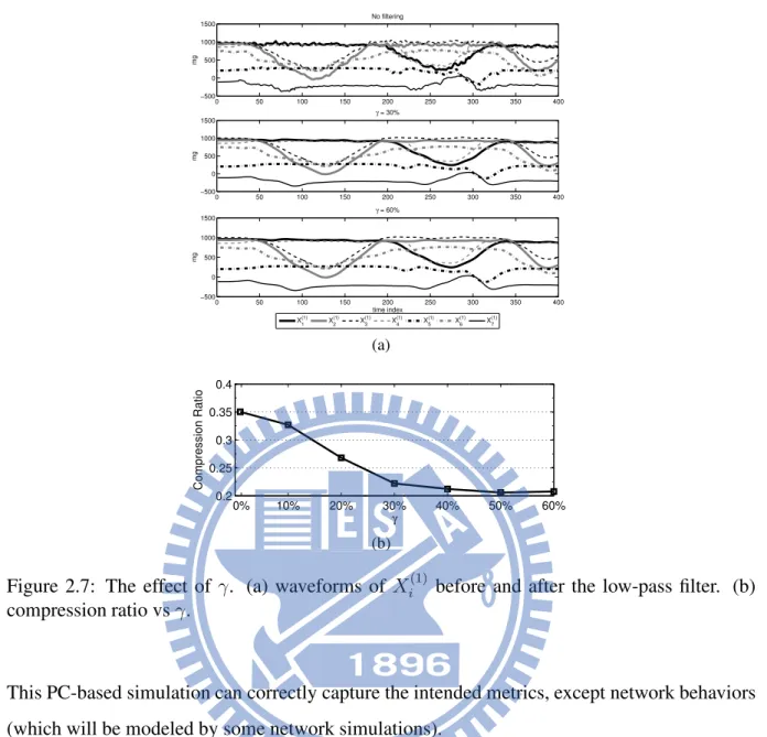
2.5.2 Effects ofγ . . . 31
2.5.3 Compression Ratio under Ideal Channel Condition . . . 32
2.5.4 Compression Ratio under Non-Ideal Channel Condition . . . 32
2.5.5 Energy Cost . . . 36
2.5.6 Scalability Issue . . . 39
2.5.7 Effect of System Retraining . . . 39
2.6 Conclusions . . . 40
3 Exploiting Multi-Spatial Correlations of Motion Data for Data Compression 42 3.1 Introduction . . . 42
3.2 Multi-Spatial Data Compression . . . 43
3.2.1 Problem Definition . . . 43
3.2.2 Complexity Analysis . . . 45
3.2.3 A Greedy Cycle Breaker Heuristic . . . 46
3.3 Experimental Results . . . 46
3.3.1 Environment . . . 47
3.3.2 Compression under Ideal Channels . . . 47
3.3.3 Compression under Lossy Channels . . . 48
3.4 Conclusions . . . 49
4 Inertial Sensor Deployment Methods for Gravity Measurement 51 4.1 Introduction . . . 51
4.2 Related Works . . . 53
4.3 Gravity Measurement and Deployment Optimization Problems . . . 54
4.4 Optimization Heuristics . . . 56
4.4.1 Metropolis-Based Method . . . 56
4.4.2 Largest-Inter-Distance-Based Method . . . 57
4.5 Simulation and Experimental Results . . . 61
4.5.1 Simulation Setup . . . 62
4.5.3 Effects of the Number of Sensors . . . 64
4.5.4 Real Gravity Measurement . . . 64
4.6 Conclusions . . . 65 4.7 Appendices . . . 65 4.7.1 Proof of Theorem 4.4.2 . . . 65 4.7.2 Proof of Theorem 4.4.3 . . . 68 5 Conclusions 77 Bibliography 78 Curriculum Vitae 83
List of Tables
List of Figures
1.1 An example of a BISN-based human motion tracking system. . . 2
1.2 System architecture. . . 3
1.3 Pilates exercises for low back pain relief. . . 4
1.4 Software architecture. . . 4
1.5 Our wireless sensing platforms. . . 5
1.6 System architecture. . . 6
1.7 Software architecture. . . 7
1.8 Human body and equipment model. . . 8
1.9 Snapshots of the game. . . 9
1.10 Virtual character and camera settings in Fig. 1.9. . . 10
2.1 A BISN architecture for motion recognition. . . 13
2.2 An example of placing sensor nodes on a human body. . . 17
2.3 Examples of Pilates exercises. . . 17
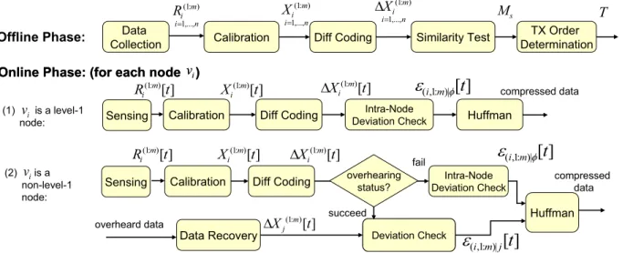
2.4 Validation of our temporal and spatial correlation modeling. (a) Calibrated data Xi(1) of exercise Fig. 2.3(a). (b) The difference vector∆Xi(1). (c) Predicting ∆X4(1)by∆X5(1). (d) Probability distribution of the prediction error vectorǫ(4,1)|5. 20 2.5 Offline and online phases of our data compression model. . . 22
2.6 An example of the MT method. . . 27
2.7 The effect ofγ. (a) waveforms of Xi(1) before and after the low-pass filter. (b) compression ratio vsγ. . . 31
2.8 Comparison of compression ratios of individual nodes (v1, v2, . . . , v7) under an ideal wireless channel. (a) exercise Fig. 2.3(a). (b) exercise Fig. 2.3(b). (c) exercise Fig. 2.3(c). (d) exercise Fig. 2.3(d). . . 33
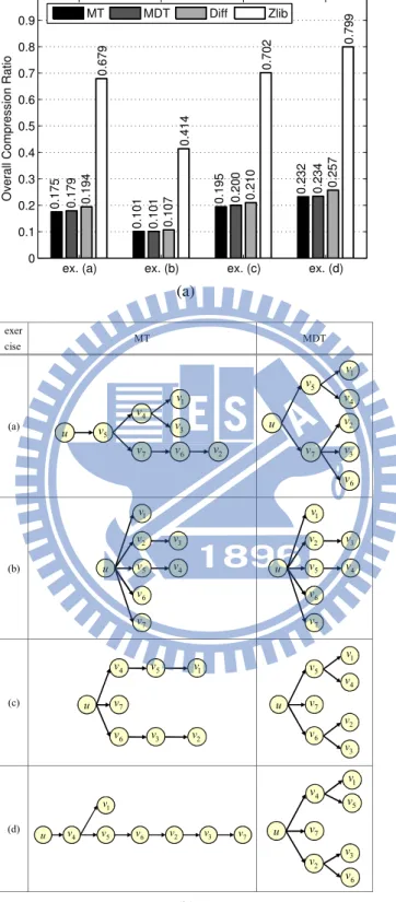
2.9 Comparison of overall compression ratios and the partial-ordering trees being used. (a) overall compression ratio. (b) partial-ordering trees. . . 34
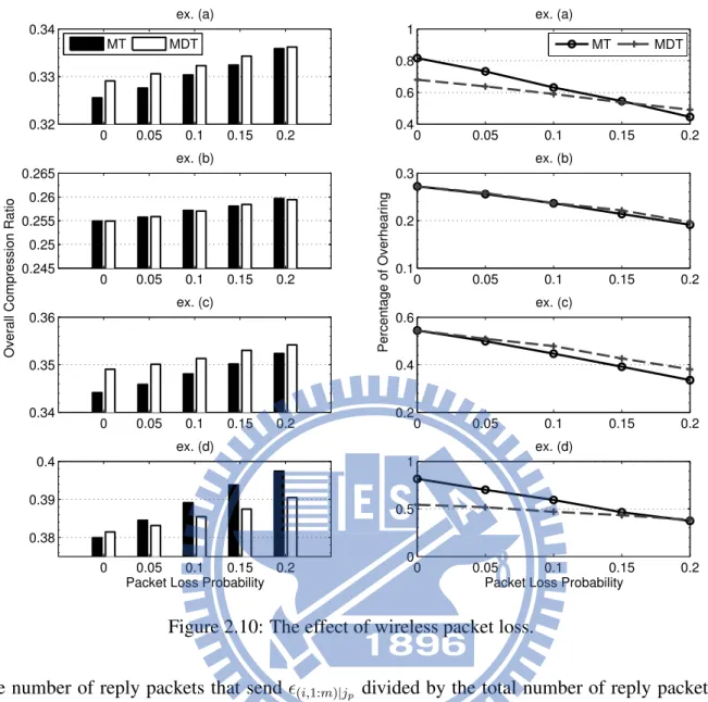
2.10 The effect of wireless packet loss. . . 36
2.11 Comparison of the maximal average per-node energy consumption among all nodes for each exercise. (a) exercise Fig. 2.3(a). (b) exercise Fig. 2.3(b). (c) exercise Fig. 2.3(c). (d) exercise Fig. 2.3(d). . . 38
2.12 The effect of system retraining on overall compression ratio. (a) exercise Fig. 2.3(a). (b) exercise Fig. 2.3(b). (c) exercise Fig. 2.3(c). (d) exercise Fig. 2.3(d). . . 40
3.1 Data compression models. c(vi| Si) means the compressed size of vi’s data aftervi overhearsSi. (a) individual. (b) single-spatial. (c) multi-spatial. . . 44
3.2 An example of 2-MDC: (a)G, (b) all dependency relations, (c) a possible DAG G′, and (d) a topological sort ofG′. . . . 44
3.3 The sensor locations in our experiments. . . 47
3.4 The distributions ofc(v| S) by |S|. . . 48
3.5 Comparison of compressed data sizes under ideal channels. . . 48
3.6 Comparison of compressed sizes under lossy channels. (a) static channels. (b) dynamic channels. . . 49
3.7 Percentage of overhearing under static lossy channels. . . 50
4.1 Gravity measurement in (a) a car and (b) a human body, whereg is the gravity vector. . . 52
4.2 The geometrical model of our work, wherev and φ are unknown to our system andg is to be calculated. . . 53
4.3 The kinematical model for one rigid body. . . 54
4.4 (a) a sphere rigid body attached by three fixed sensors and one moving sensor and (b) the reciprocals1/σ2 e(P ) by moving point p4. . . 58
4.5 (a) a cube rigid body attached by three fixed sensors and one moving sensor and (b) the reciprocals1/σ2 e(P ) by moving point p4. . . 59
4.6 A rectangular box attached by four sensors with its joint at×. . . . 60
4.7 An example of iterative projection on three consecutive polygons. . . 62
4.8 An example of running the LID-based method by Unity. (a) initial deployment. (b) final deployment. . . 62
4.10 Comparison ofα, with 95% confidence intervals shown on the bars. (a) geom-etry (a). (b) geomgeom-etry (b). (c) geomgeom-etry (c). (d) geomgeom-etry (d). (e) geomgeom-etry
(e). . . 69
4.11 Comparison ofσ2
e, with95% confidence intervals shown on the bars. (a) geom-etry (a). (b) geomgeom-etry (b). (c) geomgeom-etry (c). (d) geomgeom-etry (d). (e) geomgeom-etry (e). . . 70
4.12 Comparison of execution time. . . 71
4.13 Effects of m on α. (a) geometry (a). (b) geometry (b). (c) geometry (c). (d) geometry (d). (e) geometry (e). . . 72
4.14 Effects of m on σ2
e(P ). (a) geometry (a). (b) geometry (b). (c) geometry (c). (d) geometry (d). (e) geometry (e). . . 73
4.15 Effects ofm on execution time. (a) geometry (a). (b) geometry (b). (c) geome-try (c). (d) geomegeome-try (d). (e) geomegeome-try (e). . . 74 4.16 Our experimental scenario: (a) geometry model, (b) state “up”, and (c) state
“down”. . . 75
4.17 The angles betweenˆg(t) and the axes. (a) a slow rotation. (b) fast rotations. . . 75 4.18 The SVD process for a regular triangle. . . 76
Chapter 1
Introduction
1.1
Backgrounds and Motivation
The advance of micro-electro-mechanical systems (MEMS) and wireless communication has boosted body-area sensor networks (BSNs), in which miniature, integrated wireless sensor
nodes are deployed on a human body to monitor various physical and biological signs, such
as motion, heartbeat rate, and blood pressure [1]. An important application of BSNs is to track
human body motions by deploying inertial sensors on movable body parts, forming a body-area
inertial sensor network (BISN).
An example of a human motion tracking system based on a BISN is shown in Fig. 1.1.
The system senses a user’s motion, analyzes it, understands the intention of the motion, and
provides proper feedback to the user. The BISN, the front-end of the system, includes wireless
inertial sensor nodes deployed on the user’s body and a wireless sink node that collects sensing
data from the network. The application system analyzes the collected sensing data for various
purposes and is usually connected to peer systems and servers on the Internet for remote social
interaction and monitoring.
The use of BISNs has many advantages over traditional camera-based motion capturing
systems. It is much cheaper, immune to the line-of-sight problems in camera-based systems,
easier to track the motion of multiple users, and easier to protect user privacy. Besides, it can
be easily integrated with other types of sensors to provide more body information. Hence, BISNs have become a promising technology for a variety of applications, including pervasive
video games [2, 3], medical care [4, 5], sports training [6], affective computing [3], and
human-computer interface [7].
To boost this emerging technique, many fundamental issues need to be addressed. We list some of them as follows.
Sink
Feedback and Application System Body-Area Inertial Sensor Network
Sensor Node
Internet
Server Peer System
Local Application System
Figure 1.1: An example of a BISN-based human motion tracking system.
• Data collection. Applications may require real-time and high-resolution sensing data for various purposes, such as visualizing motions, recognizing body conditions, and di-agnosing motion disorders. These requirements imply shorter transmission delays and
higher sampling rates for a BISN. In addition, due to the size of a human body, nodes
are typically dense and almost fully connected, leading to severe contention and collision
among their transmissions [8,9]. Since wireless bandwidths are limited, how to efficiently
utilize them is very important.
• Motion tracking. The fidelity of motion tracking has critical impacts on user experience and application performance. However, due to the complexity and uncertainty of human
motion, improving it is a hard task. Issues and challenges include sensor calibration,
sensing data fusion, sensor deployment, and the design of tracking algorithms.
• Wearable sensor design. The ease of wearing is one of the major concerns in adopting wearable sensors. Besides making sensors as small and light as possible, some research
has considered how to weave them into clothes. It is also a challenging task to integrate
sensors of multiple modalities into a single system on chip (SoC). In addition to
chal-lenges in hardware manufacturing, many issues arise when sensors are miniaturized. For
example, the greatly constrained battery power may reduce network lifetime, the simplic-ity of miniaturized hardware may imply little computing power, and a shortened antenna
may have a much shorter transmission range.
• Energy saving and supply. It is desirable to prolong the network lifetime as much as possible. Recharging batteries is typically quite inconvenient or even impossible when sensors are implanted in human bodies. Therefore, how to save energy is a critical issue
Internet
Remote assisted physical rehabilitation
Exercise Date:2008/02/01
Mission: Upstairs
Steps: 86 Fail: 15 Times Act烉Climb at least 100 steps
R Leg: 18.7 Left Leg: 20 RMS Leg Angle Pressure in Gait R Foot L Foot Self-physical-rehabilitation System Sensor Upstairs Test 60 Scores:
R Up: Correct L Up: Incorrect
Figure 1.2: System architecture.
in the design of BSNs, from hardware to software. On the other hand, some research
considers how to scavenge energy from the environment to replenish battery capacity.
Putting all these together, in the following, we build some prototypes to demonstrate novel
application scenarios as well as to motivate our research.
1.1.1
Prototyping Experience: Home Rehabilitation
The BISN technology brings new light to medical care and telerehabilitation. As the aging
population has increased significantly in the past decades, long-term health care has posed an
increasing load for therapists and become an important challenge in the society. Traditionally,
physical rehabilitation programs are instructed and monitored by therapists in the hospital, and
thus consume severe medical resources. Furthermore, since the rehabilitation process is
typ-ically lengthy and boring, many patients may be reluctant to take it, thus further reducing its
effectiveness.
In this prototyping, we demonstrate a system that uses intelligent sensors to capture human
motion for home rehabilitation. Fig. 1.2 shows our system architecture. Here we consider a
set of Pilates exercises for low back pain relief (refer to Fig. 1.3) as suggested by the therapists
in Wan-Fang Hospital, Taipei. For each exercise, the graphical user interface will instruct the
patient to wear sensors at appropriate body parts.
Fig. 1.4 shows the software architecture. The system consists of three parts: a wireless
sensing platform, a motion analysis module, and a game interface. A patient needs to wear
sensors on specified body parts. The motion analysis module evaluates the quality of a patient’s movements and gives feedback through the game interface.
ʻ˴ʼ
ʻ˶ʼ
ʻ˵ʼ
ʻ˷ʼ
Figure 1.3: Pilates exercises for low back pain relief.
Tri-axial Accelerometer Electrical Compass Calibration Calibration Node
Driver Orientation Matrix
Wireless Module Wireless Module Rule Set Motion Reconstruction Recognition Motion Analysis Module Audio
User Instruction Graphics
Score Log 1 a 2 a 3 a 4 a Game Interface (g g gx, y, z) qc Sink b g Node Node Sink
Figure 1.4: Software architecture.
Wireless sensing platform. We have tested two platforms: Octopus II and ECO systems
(refer to Fig. 1.5). Octopus II is modified from the Tmote Sky system [10] and runs TinyOS,
while ECO [11] is quite tiny and is extremely resource-limited. Both platforms use the TDCM3
electrical compass. Octopus II uses the FreeScale MMA7260QT accelerometer and ECO uses
the Hitachi-Metal H34C accelerometer. These triaxial accelerometers can capture the gravity in
x, y, z-axes. Note that a compass is needed since the rotation angle about the gravity cannot be inferred from the accelerometer along. Octopus II uses a TDMA protocol provided by TinyOS
to increase data rate. On the other hand, ECO adopts a simple polling protocol. On the sink side,
the accelerometer and compass readings from each node are further combined into orientation
matrices in the world coordinate.
Motion analysis module. This module takes the accelerometer readings and the orientation
(a) ECO system (b) OctopusII system
Figure 1.5: Our wireless sensing platforms.
motions is the joint angle information (α1, . . . , α4 in Fig. 1.4). Another is the angle between each sensor node and the gravity direction (β in Fig. 1.4). Our scoring mechanism analyzes these parameters to judge if the patient’s performance is acceptable or not. For instance, the
patient is considered to perform exercise (a) in Fig. 1.3 well if (1) the joint angle between two
legs is around 45◦, and (2) the movement of his pelvis is within a small range. Item (1) is implemented by restricting the joint angle within45◦ ± 10◦, and item (2) by restrictingβ, the angle between the frontal plane and the gravity direction, within a small range.
Game interface. This layer interacts with the user and stores the results of each exercise.
The game has multiple levels, each as one Pilates exercise. The game will create some events, and the patient should react by performing the specified Pilates exercise. The game interface
queries the motion analysis module to check if the patient’s performance is acceptable, and if
so, some rewards are given. The patient should get enough rewards to pass a level. Most of
the hints are shown on the screen, but if the patient cannot watch the screen in some Pilates
exercises, audio hints will be given instead.
In our demonstration, we show exercises (a) and (b) using Octopus II and ECO, respectively.
In exercise (a), the game is to open a treasure box. The player should raise his leg to about45◦ to open the lid and collect at least five treasures to pass this level. In exercise (b), the player
should keep his knee joint angle to about90◦and raise two legs up simultaneously.
1.1.2
Prototyping Experience: Multi-Screen Cyber-Physical Video Game
Cyber-physical systems (CPS)have drawn a lot of attention recently. In the past two decades, cyber systems were one of the fastest growing areas due to the advance of mobile computing technologies (such as portable computers and smart phones) and the standardization of
vari-Wired LAN North Screen SouthScreen East Screen : Game Engines West Screen Sink : Inertial Sensors 1 G 1, 2, 3, 4 G G G G 2 G 3 G 4 G
: Cyber-Physical Game Controller
c c 1, 2, ,3 4 v v v v 1 v 2 v 3 v 4 v
Figure 1.6: System architecture.
ous wireless communication and networking technologies (such as ZigBee, WiFi, Bluetooth,
WiMAX, 2G/3G/3.5G, LTE, etc.), which are tightly integrated under the Internet environment.
On the other hand, a major advance in physical systems is the development of
micro-electro-mechanical systems (MEMS), which can greatly enrich cyber systems with more physical inputs and actuators.
We are interested in CPS for cyber-physical video games. Traditionally, cyber video games
are supported by game engines that take players’ inputs from keyboards and joysticks. Enhanc-ing such systems with more physical inputs, such as body motions captured by inertial sensors,
has attracted a lot of attention recently. We call such systems cyber-physical games. The
Nin-tendo Wii [2] is one example with MEMS-based inertial sensors. Reference [7] shows that by
using MEMS-based inertial sensors and a wired network, body motions can be reconstructed
through computer animation with little distortion. Wireless-based body-area inertial sensor
networks (BISNs)have been studied in [12]. On the other hand, new display technologies, such as LCD, plasma, and back-projection displays, can further enrich cyber-physical games with
better visual effects [13].
The above advances motivate us to develop a multi-screen cyber-physical video game with
physical inputs from players equipped with BISNs. We demonstrate our prototype of the BISN platform, the Cyber-Physical Game Controller, and the Game Engines.
single-Triaxial Accelerometer Triaxial Electronic Compass Calibration Calibration Sensor Nodes Wireless Communication Wireless Communication Sink Compression Compression Orientation Matrix Cyber-Physical Game Controller Decompression Human Body and Equipment Model
Game Engines Input Dispatcher 1 v v2 Graphics Library (OpenGL ) Event Handler Network Input Common Scene Data Local Profile Game Ke rnel BISN Platform 3 v 4 v 3 G Graphics Library (OpenGL ) Event Handler Network Input Common Scene Data Local Profile Game Kernel 4 G Event Handler Network Input 1 G Common Scene Data Local Profile Game Kernel 2 G Graphics Library (OpenGL) Event Handler Network Input Common Scene Data Local Profile Game Kernel Graphics Library (OpenGL) Polling MAC Polling
MAC AccelerometerTriaxial Triaxial Electronic Compass Calibration Calibration Wireless Communication Compression Compression . .. Triaxial Accelerometer Triaxial Electronic Compass Calibration Calibration Wireless Communication Compression Compression . .. Triaxial Accelerometer Triaxial Electronic Compass Calibration Calibration Wireless Communication Compression Compression . ..
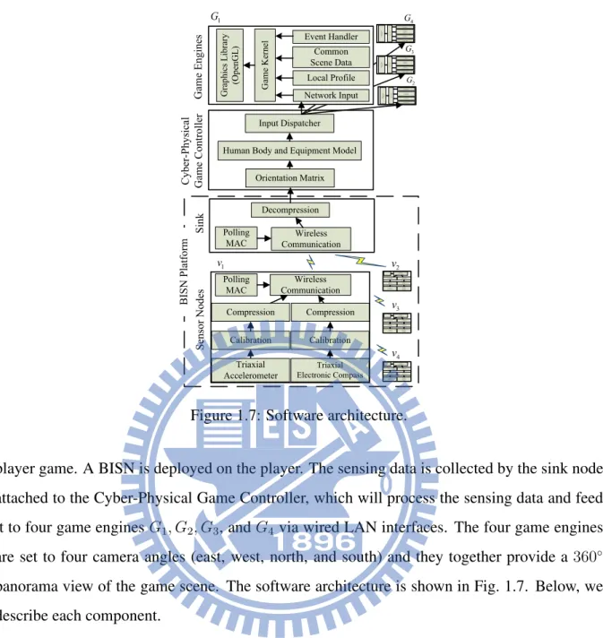
Figure 1.7: Software architecture.
player game. A BISN is deployed on the player. The sensing data is collected by the sink node
attached to the Cyber-Physical Game Controller, which will process the sensing data and feed it to four game enginesG1, G2, G3, andG4 via wired LAN interfaces. The four game engines are set to four camera angles (east, west, north, and south) and they together provide a360◦ panorama view of the game scene. The software architecture is shown in Fig. 1.7. Below, we
describe each component.
BISN platform. The platform consists of one sink node and four inertial sensor nodes
v1, v2, v3, andv4. Each node consists of some inertial sensors, a micro-controller, and a wireless module. In our current implementation, each node is equipped with a triaxial accelerometer and a triaxial electronic compass. The triaxial accelerometer senses the gravity in x, y, and
z-axes, while the triaxial compass senses the earth magnetic force in x, y, and z-axes. The
“Calibration” module removes noises and converts sensing signal into meaningful data. Since
sensing data is streaming data, the “Compression” module executes a differential coding to
reduce data transmission. The compressed data is reported to the sink through the “Wireless
Communication” module. The sink node runs a “Polling MAC” to avoid collisions and to
improve throughput.
Jennic JN5139
Cell-phone Battery Inertial Sensor (OS5000)
Öx Sensor Axis Öx Öy Öz East North Up Orientation Matrix Sensor Coordinate Earth Coordinate Öx Öy Öz Öx Öy Öz Öx Öy Öz 1
T
T
2 ÖyÖx
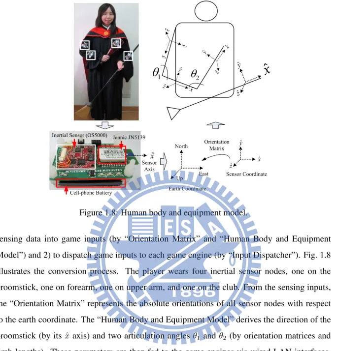
ÖzFigure 1.8: Human body and equipment model.
sensing data into game inputs (by “Orientation Matrix” and “Human Body and Equipment
Model”) and 2) to dispatch game inputs to each game engine (by “Input Dispatcher”). Fig. 1.8
illustrates the conversion process. The player wears four inertial sensor nodes, one on the
broomstick, one on forearm, one on upper arm, and one on the club. From the sensing inputs,
the “Orientation Matrix” represents the absolute orientations of all sensor nodes with respect
to the earth coordinate. The “Human Body and Equipment Model” derives the direction of the
broomstick (by itsx axis) and two articulation angles θ1ˆ and θ2 (by orientation matrices and limb lengths). These parameters are then fed to the game engines via wired LAN interfaces.
Typical game engines do not support multiple screens. Our game controller tries to simulate a multi-screen game engine by sending proper data, via the “Input Dispatcher” to four game
engines, as explained below.
Game engines. Each game engine has a “Game Kernel”, which takes inputs from four
modules. The “Common Scene Data” module describes the virtual world. It is the same for all
game engines. The “Network Input” module receives game inputs from the “Cyber-Physical
Game Controller” and updates the virtual world in the game. The “Event Handler” module
processes the interactions, especially collisions, between virtual objects and the player. For
example, when the player hits a ball, it bounces away, and the “Event Handler” increases the player’s score. Each game engine contains a camera, whose direction is specified by the
“Lo-(a) (b)
Figure 1.9: Snapshots of the game.
cal Profile”, that takes pictures for its virtual world and feeds the captured data to the “Game
Kernel”, which calls the “Graphics Library” to display the results. Since we have four game engines with four cameras facing to east, west, north, and south, a360◦ panorama view of the virtual world is provided to support better visual effect to the player.
Demonstration.We adopt the Quidditch sports in “Harry Potter” as our game scenario. The player rides a flying broom in a practice field, and she tries to attack approaching balls by her
club. She flies at a constant speed and controls her broomstick to change directions.
For the BISN platform, we adopt Jennic JN5139 [14] and OS5000 sensor [15] (refer to
Fig. 1.8). Each Jennic JN5139 consists of a micro-controller and a IEEE 802.15.4 wireless
transmission module, and each OS5000 has a triaxial accelerometer and a triaxial electronic
compass. The sampling rate is set to 20Hz, a common value for motion capturing [16]. The average packet loss rate of our polling MAC is about0.16%, and the average delay for collecting a complete set of sensing data from a node is around 83 ms.
Fig. 1.9 shows some snapshots of the game. The player flies a short distance to the north
in Fig. 1.9(a), and then she turns to the west in Fig. 1.9(b). We adopt Unity [17] as our game
engine, which features a fully integrated editor and a physics engine for rapid 3D game
proto-typing. Fig. 1.10(a) and Fig. 1.10(b) show the corresponding settings of the west and the north
game engines in Fig. 1.9(a), respectively. The virtual character, who is controlled by the player,
looks to the north in both game engines. The camera of Fig. 1.10(a), whose viewing volume is
illustrated by white lines, looks to the west, while the camera of Fig. 1.10(b) looks to the north.
Fig. 1.10(c) and Fig. 1.10(d) correspond to the west and the north screens in Fig. 1.9(b),
respec-tively, where both of the player and the virtual character look to the west, but the directions of the cameras remain unchanged.
(a) (b)
(c) (d)
Camera attached on the character
Border of viewing volume Camera position and rotation
Light
Figure 1.10: Virtual character and camera settings in Fig. 1.9.
1.2
Issues Addressed in this Dissertation
We conduct fundamental research into the technologies required to create an efficient wireless
communication BISN that maximizes tracking accuracy and spectrum efficiency. Specifically,
we conduct three pieces of research. The first work addresses the data collection issue by data
compression by exploiting temporal-spatial correlations of sensing data. Based on the first work, the second work considers multi-spatial correlations of motion data to better exploit
pos-sible spatial correlations. In the third work, we address a fundamental issue in motion tracking,
the gravity measurement problem. Below, we briefly describe each piece of our research.
Concerning that human bodies are relatively small and wireless packets are subject to more
serious contention and collision, the first work of this dissertation addresses the data
compres-sion problem in a BSN. We observe that, when body parts move, although sensor nodes in vicinity may compete strongly with each other, the transmitted data usually exists some
lev-els of redundancy and even strong temporal and spatial correlations. Unlike traditional data
compression approaches for large-scale and multi-hop sensor networks, our scheme is
specifi-cally designed for BSNs, where nodes are likely fully connected and overhearing among sensor
nodes is possible. We model the spatial-temporal data compression problem, where overhearing
should be efficiently utilized, as a combinatorial optimization problem on graphs, showing its
hardness, and presenting efficient algorithms to approximate optimal solutions. We also discuss
the design of the underlying MAC protocol to support our compression model. An experimental
case study in Pilates exercises for patient rehabilitation is reported. The results show that our schemes reduce more than70% of overall transmitted data compared with existing approaches.
The first work has shown how to compress motion data by allowing a node to overhear at
mostκ = 1 node’s transmission and exploit the correlation with its own data for data compres-sion. In the second work, we consider multi-spatial correlations by extendingκ = 1 to κ > 1 and constructing a partial-ordering directed acyclic graph (DAG) to represent the compression
dependencies among sensor nodes. While a minimum-cost tree forκ = 1 can be found in poly-nomial time, we show that finding a minimum-cost DAG is NP-hard even forκ = 2. We then propose an efficient heuristic and verify its performance by real sensing data.
In addition to data collection, in the third work, we are interested in tracking human postures
by deploying accelerometers on a human body. One fundamental issue in such scenarios is how
to calculate the gravity. This is very challenging especially when the human body parts keep
on moving. Fortunately, it is likely that there is a point of the body that touches the ground
in most cases. This allows sensors to collaboratively calculate the gravity vector. Assuming
multiple accelerometers being deployed on a rigid part of a human body, a recent work proposes
a data fusion method to estimate the gravity vector on that rigid part. However, how to find
the optimal deployment of sensors that minimizes the estimation error of the gravity vector is not addressed. In this work, we formulate the deployment optimization problem and propose
two heuristics, called Metropolis-based method and largest-inter-distance-based (LID-based)
method. Simulation and real experimental results show that our schemes are quite effective in
finding near-optimal solutions for a variety of rigid body geometries.
To summarize, there are four significant innovations that resulted from this research:
1. Greatly improved spectrum efficiency of the wireless communications in a BISN by
us-ing spatial-temporal data compression on sensus-ing data. This is accomplished by
exploit-ing the spatial-temporal features inherent in human body motions and createxploit-ing a data compression methodology that resulted in an energy-efficient, low-delay communication
protocol that is suitable for real-time, accurate human motion capturing.
2. The theoretical findings that show the sharp increase in the computational complexity
of exploiting spatial correlations. The optimal data compression scheme can be found in
polynomial time when each node is restricted to overhear up to one other node; otherwise,
allowing overhearing more nodes makes finding an optimal data compression scheme a
NP-hard problem. We propose efficient heuristics to solve the NP-hard problem. The hardness results also apply to other types of WSNs.
3. The inertial sensor deployment scheme that maximizes tracking accuracy. Intuitively
speaking, we place sensors on different locations of a target body part to
collabora-tively capture more information about its motions. We model the kinematics of sensors’
readings and propose algorithms to find optimal deployments that capture the maximal
amount of information, which can be fused to improve tracking accuracy.
4. The development of innovative applications using the motion tracking system to
demon-strate its capabilities and to serve as a proof of concept for the technology in a variety of
consumer usage models.
• A cyber-physical video game where the user is able to control the game in a body-intuitive way, and is able to control the panoramic view of the game scenes in a
sensor-controlled way.
• A remote physical rehabilitation system that enables patients to avoid having to wait for rehabilitation appointments in the hospital, eliminating travel time, and reducing
demands for medical resources.
1.3
Organization of this Dissertation
The rest of dissertation is organized as follows. Chapter 2 addresses data collection issues by
exploiting data compression by taking advantage of the spatial-temporal features of sensing
data when sensors are deployed on a human body and the possibility that sensors can overhear
each others’ transmissions in a BISN. Based on Chapter 2, Chapter 3 consider multi-spatial
correlations of motion data for data compression. Besides data collection, Chapter 4 addresses
a fundamental issue in human motion tracking, the gravity measurement problem. Chapter 5
Chapter 2
Data Compression by Temporal and
Spatial Correlations in a BISN
2.1
Introduction
In Section 1.1.1, we have demonstrated applying BISNs to physical rehabilitation, where pa-tients have to frequently practice certain fixed-pattern exercises repeatedly [5]. Such a scenario
can be shown as in Fig. 2.1, where a BISN is deployed on a patient to capture her body
mo-tions. Via wireless links, the sink is able to collect sensing data, the data analyzer is able to
analyze and visualize her motions, and the application system is able to give comments and
send feedbacks to therapists for further diagnosis.
Such applications may require real-time and high-resolution sensing data for various
pur-poses, such as visualizing motions, recognizing body conditions, and diagnosing diseases.
These requirements imply shorter transmission delays and higher sampling rates for the BISN.
In addition, due to the size of a human body, nodes are typically dense and almost fully con-nected, leading to severe contention and collision among their transmissions [8, 9]. Since
wire-less bandwidths are limited, how to efficiently utilize them is very important.
We attack these issues by exploiting data compression by taking advantage of the special
Internet
Sink Data Analyzer
Feedback and Application System
features of sensing data when sensors are deployed on a human body and the possibility that
sensors can overhear each others’ transmissions in a BISN. We observe that when human body
parts move, it usually exhibits strong temporal and spatial correlations among sensing data.
By temporal correlation, body signs sensed by a single node typically change smoothly and
slowly. By spatial correlation, body signs measured on different nodes are typically correlated because body components are connected and they normally move with certain rhymes. On the
other hand, since nodes in a BISN are typically fully connected, spatial correlations can be
efficiently exploited through overhearing, a nature of wireless communication, among nodes
to minimize the total amount of transmissions. Although data compression schemes that
ex-ploit temporal and spatial correlations in wireless sensor networks (WSNs) have been widely
discussed [18, 19], such schemes are usually designed for large-scale networks with multi-hop
communications and are thus not suitable for BISNs, which are likely fully connected,
provid-ing a room for customized data compression of body motion data.
Since wearable devices are typically lightweight and have limited computation power and
resources, the corresponding sensing data processing, compression, and MAC protocol should
be lightweight, too. In particular, the following guidelines are important in designing data
com-pression schemes for BISNs. First, the general form to model the temporal-spatial correlations
of human body parts should not be too complicated, especially when considering the correlation among multiple sensors on different nodes. Second, we have to take the data gathering process
and the distributed nature of a BISN into consideration. For example, the rich connectivity of a
BISN normally incurs higher contention and collision among transmissions.
In this chapter, we propose a novel data compression method for BISNs based on over-hearing. We exploit temporal and spatial correlations among sensing data to facilitate data
compression and transmissions. Each node samples its data, overhears others’ transmissions,
compresses its data, and then transmits. Temporal and spatial correlations are modeled by
dif-ferential coding and linear regression, respectively. Note that our data compression is lossless.
In our method, an offline phase is conducted to learn these correlations and various system
parameters. Then, nodes are sorted into a partial ordering tree, which specifies the preferred
transmission order of nodes (level-1 nodes transmit first, followed by level-2 nodes, etc.).
Dur-ing the online phase, each node overhears others’ transmissions, decodes some of them, encodes
its own sample according to the learned correlations, and transmits the encoded result. It is to be noted that under our modeling, the compression ratio is indeed affected by nodes’
transmis-sion order. Our scheme can also tolerate that the actual transmistransmis-sion deviates from the ideally
planned order, at the cost of a higher compression ratio. We show how to construct an optimal
partial-ordering tree, called Minimum-Cost Tree (MT), such that the total data transmitted on the
air is minimal statistically. The MT scheme, however, may need to decode and encode a long
sequence of overheard data. An alternative is a near-optimal Minimum-Cost, Depth-Bounded
Tree (MDT), which limits the number of transmissions to be overheard by each node. The MDT scheme is more practical, but unfortunately, it has been proven that optimizing tree cost given
any bound on its depth is NP-hard.
To summarize, major contributions of this chapter are three-fold. First, a distributed data
compression method suitable for BISNs is proposed to exploit temporal and spatial correlations
of sensing data. Our method considers the correlation among multiple sensors on different
nodes. The computation complexity and communication overhead are kept as low as possible.
Second and more importantly, we utilize overhearing, a nature of wireless communication, and investigate the prediction directions in spatial correlations. We show how to construct
an optimal partial-ordering tree, based on which nodes can sent their transmission sequences
and overhear others’ transmissions in a cooperative way so as to minimize the total amount of
transmissions. To the best of our knowledge, applying overhearing in data compression is never
explored before. We also propose a more practical minimum-cost, depth-bounded tree, which
turns out to be NP-hard. These techniques may be applied to other distributed source coding,
too. Third, to verify our results, an experimental case study in Pilates exercises for patient
rehabilitation is reported.
The rest of chapter is organized as follows. Section 2.2 reviews some related works. Section
2.3 describes our BISN system architecture. Section 2.4 gives our data compression models and
algorithms, including some notes on practical issues. Experimental results and our prototypes
are shown in Section 2.5. Section 2.6 concludes this chapter.
2.2
Related Works
BSN is an emerging technique. Its bandwidth utilization issues have started to receive attention.
Assuming a fully connected BSN, a QoS framework similar to IEEE 802.16 is proposed for
BSNs in [20] to grant connections and allocate bandwidths based on applications’ requests.
Several lossy data compression methods have been proposed. In [21], sensors with higher priorities are allowed to transmit their sensing data with higher precision. If the data sources
are sparse, e.g., in the case of PPG signals, compressed sensing techniques can be applied to
reduce the required sampling rates [22]. For motion capturing, [12] has tested the performance
of several existing lossless and lossy compression algorithms on motions that exhibit repetitive
patterns, such as running. However, the compression is performed by each individual sensor and
does not consider the correlations among sensors. We extend their work to consider correlations among sensors (both on the same node and on different nodes). Although our data compression
model is lossless, any lossy transform (e.g., FFT and wavelet transform mentioned in [12])
can be applied to the data source before passing through our data compression model. If the
application is interested only in certain events, rather than the sensing values, distributed motion
classification/annotation would be most efficient [23, 24].
On the other hand, for large-scale WSNs, data compression has been intensively studied.
We classify these solutions as follows.
• Cross-layer solutions. The impact of joint routing and compression is studied in [25]. Reference [26] studies the feasibility of sublinear scaling laws under different cooperation
schemes for spatially correlated data.
• Data aggregation. Data compression may be performed by relay nodes or cluster heads via data aggregation. TAG [27] organizes a network into a tree and proposes SQL-like
semantics to aggregate streaming data into histograms for low-power aggregation.
Multi-resolution spatial and temporal coding is addressed in [28].
• Data acquisition. As acquiring sensing data from a large-scale WSN to a user’s hand-held device may involve long delays, non-uniform energy consumptions, and network
impairments, model-driven data acquisition models are proposed in [18,19,29]. Although
these methods are suitable for infrequent queries and slow-changing environments, they
are not practical for motion capturing, as motion data usually changes more rapidly.
2.3
BISN System Architecture
We consider a BISN deployed on a human body for motion recognition. An example is the
Pilates exercises for patient rehabilitation. The system architecture is shown in Fig. 2.1.
Wear-able sensor nodes are placed at main movWear-able body parts. These nodes will periodically report their readings to a sink node, which is connected to the data analyzer. The data analyzer will try
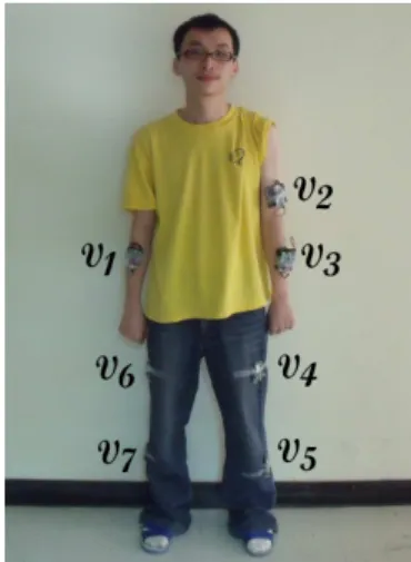
Figure 2.2: An example of placing sensor nodes on a human body.
Figure 2.3: Examples of Pilates exercises.
to understand how well the person conducts some motions. The application server can further
send feedbacks to the person and reconstruct, store, and replay these motions.
As an example, to recognize Pilates exercises for lower back pain relief [30, 31], nodes can
be placed at main body parts as shown in Fig. 2.2. Some Pilates exercises are shown in Fig. 2.3.
In the upper leg lifting exercise (b), one has to lie on his side and put legs and feet together in parallel. Then, lift the top leg up from 0◦ to about 45◦, stay for about 5 seconds, and then return to the start. The exercise needs to be repeated several times.
Due to the size of a human body, nodes in a BISN are typically fully connected.
There-fore, when a node is transmitting, the other nodes can overhear its transmission. In addition,
their data could be highly correlated. By utilizing the overheard information, one may
con-duct compression based on sensor data’s spatial and temporal correlations. We show that by
properly arranging nodes’ transmission order, not only the competition and interference among nodes can be relieved, but also significant compression can be done. In this work, we place a
triaxial accelerometer in each sensor node. The sampling rate on each axis is set to 20 Hz, a
common value for body motion measurement [16]. (However, the applicability of our work is
not limited to these assumptions.) Sensor readings are calibrated and compressed locally, but
the computation should be kept as simple as possible.
2.4
Design of Data Compression by Overhearing
We first present our basic idea in Section 2.4.1. Then we present our data compression model
and two algorithms to sort nodes’ overhearing sequences in Section 2.4.2 and Section 2.4.3,
respectively. Although our model does not require to change the underlying MAC protocol, we
discuss the corresponding design issues in Section 2.4.4. Finally, in Section 2.4.5, we discuss
how to retrain the system where there are deviations between the training parameters and the actual behaviors.
2.4.1
Basic Idea
We consider a BISN withn nodes v1, v2, . . . , vn, each equipped withm sensors. Note that in the case of triaxial accelerometer, each axis is regarded as one separate sensor. We will design
a compression scheme to exploit the temporal and spatial correlations of sensor readings. The
goal is to automatically learn these correlations to facilitate compression. Our system has an
offline phaseand an online phase. During the offline phase, we will collect the raw outputs of thejth sensor of vi into a column vectorR(j)i , where thetth sampling result is stored at the tth entry in the vector and is written as R(j)i [t]. Note that since the same Pilates exercise should be repeated multiple times by the same person to make the training results more representative, R(j)i should contain the result of several repetitions of the same Pilates exercise. Then Ri(j)is calibrated into a column vectorXi(j)of the same size carrying meaningful data. Note that we do not specify the size of vectorR(j)i . A larger vector means more statistics, leading to higher accuracy in our prediction of correlations.
Temporal correlation hereby means the similarity of sensing values over the time axis, i.e., ∆Xi(j)[t] = X
(j)
i [t]− X (j)
i [t− 1] is very likely to fall within a small range relative to that of the original valueXi(j)[t]. Previous researches [12,16] also show that body movements are normally centered at very slow frequencies and do not change rapidly in nearby samples.
Spatial correlation hereby means that human motions in nearby body parts show inherent rhythm, making it a good source for data compression. Specifically, one may easily predict
∆Xi(1), ∆Xi(2), . . . ,∆Xi(m) given ∆Xk(1), ∆Xk(2), . . . ,∆Xk(m), if nodesvi andvk are attached to correlated body parts. To achieve low-complexity compression, we would investigate the
possibility of establishing the following linear correlation:
∆Xi(j)= α(i,j)|k1+ β(i,j)|(k,1)∆Xk(1)+
β(i,j)|(k,2)∆Xk(2)+· · · + β(i,j)|(k,m)∆Xk(m)+ ǫ(i,j)|k,
(2.1)
whereα(i,j)|kandβ(i,j)|(k,1), . . . ,β(i,j)|(k,m)are scalars, 1 is a column vector containing all 1s, and ǫ(i,j)|kis a column vector to compensate the prediction errors. If the outputs of some sensor of vkhave little correlation with∆Xi(j), its correspondingβ should approach zero. With properly selected coefficientsα and β, vector ǫ(i,j)|kwould contain all very small values, making it much less costly to represent ǫ(i,j)|k than ∆Xi(j). The number of bits required to represent ǫ(i,1)|k, ǫ(i,2)|k, . . . , ǫ(i,m)|k is used as the cost to compress sensing data of vi when the data of vk is known. Intuitively, we try to recovervi’s data from vk’s data. In subsequent sections, we will show how to find the optimal predictorvkof each nodevi (by building a partial ordering tree) so as to minimize the overall cost.
On the other hand, sensors of the same nodevi(such as∆Xi(j)and∆X (k)
i ) may also exhibit strong spatial correlations, especially among the three axes of a triaxial accelerometer. We call
such spatial correlations intranode spatial correlations, and those among sensors of different
nodes internode spatial correlations. So Eq. (2.1) is generalized as follows to include intranode
spatial correlations: ∆Xi(j)= α(i,j)|k1+ m X p=1 β(i,j)|(k,p)∆Xk(p)+ X q∈L(i,j)|k β(i,j)|(i,q)∆Xi(q)+ ǫ(i,j)|k, (2.2)
where we use all sensors ofvk and a setL(i,j)|k of sensors ofvi to predict∆Xi(j). Note that to conduct data compression, we must avoid circular dependency among sensors of the samevi. L(i,j)|kis to specify the set of sensors ofviwhose sensing data are encoded before that of sensor j. Later on, we will show how to determine the set L(i,j)|k. By learning the intranode spatial correlations in Eq. (2.2), the resulting error vectorǫ(i,j)|k of Eq. (2.2) is expected to be even smaller than that of Eq. (2.1), making compressing the former more efficient than compressing the latter.
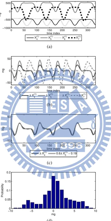
0 50 100 150 200 250 300 −1000 −500 0 500 time index mg X 4 (1) X 5 (1) X 6 (1) X 7 (1) (a) 0 50 100 150 200 250 300 −50 0 50 time index mg ∆ X4(1) ∆ X5(1) ∆ X6(1) ∆ X7(1) (b) 0 50 100 150 200 250 300 −50 0 50 time index mg ∆ X4(1) 0.6∆ X5(1) − 0.19 (c) −100 −5 0 5 10 0.05 0.1 0.15 0.2 mg Probability (d)
Figure 2.4: Validation of our temporal and spatial correlation modeling. (a) Calibrated data Xi(1) of exercise Fig. 2.3(a). (b) The difference vector∆Xi(1). (c) Predicting∆X4(1) by∆X5(1). (d) Probability distribution of the prediction error vectorǫ(4,1)|5.
Our experiences show that the above modeling is quite effective in recognizing Pilates
ex-ercises. Consider the sensor deployment in Fig. 2.2 and the exercise in Fig. 2.3(a) and
as-sume that each node has only one x-axis accelerometer. Fig. 2.4(a) shows the calibrated data X4(1), . . . , X (1) 7 . We see thatX (1) 4 and X (1)
5 exhibit strong spatial correlations, and so areX (1) 6 andX7(1). By taking the difference operation onXi(1), Fig. 2.4(b) shows that∆Xi(1)has a much smaller range, and the aforementioned spatial correlations still exist. So we can apply Eq. (2.2)
to predict∆X4(1) by∆X5(1), as shown in Fig. 2.4(c). Fig. 2.4(d) shows the corresponding prob-ability distribution of the contents of the error vectorǫ(4,1)|5. As can be seen, the distribution concentrates around 0mg.
By overhearing among sensor nodes, we will investigate the feasibility of learning these
correlations in the offline phase and exploring real-time data compression in a BISN during the
online phase. We will also address the issue of the supporting MAC protocol, especially the
design of packet collision, in Section 2.4.4.
2.4.2
Data Compression Model
Data flows of our offline and online phases are shown in Fig. 2.5. Temporal correlation will
be exploited on individual sensors by a simple differential coding, while spatial correlation
will be exploited across sensors and will be learned from the offline phase. The learned
re-sults consist of some coefficients and some transmission and encoding orders, which are sent to the sensor nodes for them to conduct online data compression. The transmission order,
which is represented by a spanning tree, specifies the partial ordering of nodes’ transmissions
and the target nodes that a node should overhear. To simplify the notations, we will
abbre-viate R(1)i , . . . , R(m)i by R(1:m)i , ∆Xi(1), . . . , ∆Xi(m) by ∆Xi(1:m), β(j,q)|(i,1), . . . , β(j,q)|(i,m) by β(j,q)|(i,1:m), ǫ(i,1)|j, . . . , ǫ(i,m)|j by ǫ(i,1:m)|j, β(j,q)|(j,l) for all l ∈ L(j,q)|i by β(j,q)|(j,L(j,q)|i), and so on.
Offline phase. In the offline phase, for each type of motion, training data are collected from the BISN in the “Data Collection” block and then sent to an external data analyzer, where the
rest of the blocks will be executed.
Data collection. We will collect from nodes v1, v2, . . . , vn column vectors R(1:m)1 ,R2(1:m), . . . ,R(1:m)n . In the collection process, each nodevi puts thetth sampling result of its qth sensor into Ri(q)[t]. R(1:m)i should be stored in vi and then forwarded to the sink in a reliable way to avoid the impact of network impairments. The same Pilates exercise should be repeated
Calibration (1: ) 1,..., m i i n R =
Diff Coding TX Order
Determination Data Recovery Calibration ( ,1: )|i m j
[ ]
t
e
(1: ) [ ] m i R t (1: )m[ ] i X t (1: )m[ ] i X t D (1: ) [ ] m j X t D compressed dataOffline Phase: Similarity Test
s M T overheard data Diff Coding Huffman Calibration (1: ) [ ] m i R t (1: ) [ ] m i X t (1: )m[ ] i X t D compressed data
Diff Coding Huffman
Online Phase: (for each node )vi
Online Phase: (for each node )vi
(1) is a level-1 node:i v (2) is a non-level-1 node: i v Data Collection Sensing Sensing (1: ) 1,..., m i i n X = (1: ) 1,..., m i i n X = D Deviation Check Deviation Check overhearing status? fail succeed Intra-Node Deviation Check ( ,1: )|i mf
[ ]
t
e
Intra-Node Deviation Check ( ,1: )|i mf[ ]
t
e
Figure 2.5: Offline and online phases of our data compression model.
multiple times by the same person to make the training results more representative, i.e., R(j)i should contain the results of several repetitions of the same Pilates exercise. To make the learned
results effective, it is assumed that the same Pilates exercise is performed by the same person in the online phase.
Calibration. Each R(j)i , i = 1 . . . n, j = 1 . . . m, is converted into a meaningful vector Xi(j). For example, the raw outputs of an accelerometer may be converted from voltages into physical units (e.g., Guass). Then we may apply various data filtering techniques to refine the
data. For human motion, we propose to use a low-pass filter to remove noise. We adopt the
FIR filter based on Kaiser window function [32]. A low-pass filter will zero out the signal
components whose frequencies are higher than a predefined stopband frequency. As the energy
of the filtered signal components become larger, the resulting signal waveform will become smoother. To automatically determine the stopband, we apply a fast Fourier transform toR(j)i such that the removed energy is equal to γ percent of the total energy. We will test different values ofγ in Section 2.5. The filtered data are rounded to the nearest integers and recorded in Xi(j).
Diff coding. To exploit temporal correlation, each Xi(j) is converted into a differential column vector∆Xi(j)such that∆X
(j) i [t] = X (j) i [t]− X (j) i [t− 1].
Similarity test. Our goal is to identify the correlation between the outputs of each pair ofvi andvj. Specifically, ann× n similarity matrix Ms will be constructed. Ms[i][j] is to measure how well we can predict the data of vj given the data of vi. For ease of explanation, for now we assume that L(j,1:m)|i is given (we will explain how to find it later). To computeMs[i][j],
we apply Eq. (2.2) and try to build the following equality for each q = 1, 2, . . . , m, where t = 1, 2, . . . : ∆Xj(q)[t] = α(j,q)|i+ m X p=1 β(j,q)|(i,p)∆Xi(p)[t]+ X l∈L(j,q)|i β(j,q)|(j,l)∆Xj(l)[t].
Then we can computeα(j,q)|i,β(j,q)|(i,1:m)andβ(j,q)|(j,L(j,q)|i)for eachq by linear regression
analy-sis [33]. Note that linear regression only tries to use the coefficients on the right-hand side to
ap-proximate∆Xj(q)[t], so we let the difference ǫ(j,q)|i[t] = ∆Xj(q)[t]−α(j,q)|i−Pmp=1β(j,q)|(i,p)∆Xi(p)[t]− P
l∈L(j,q)|iβ(j,q)|(j,l)∆X
(l)
j [t]. Intuitively, if ∆X (1:m)
i is obtained by overhearing, we only need to transmit the difference vector ǫ(j,q)|i to obtain ∆Xj(q). Here we use the notation ǫ(j,q)|φ to represent that vi’s transmission is not based on any overhearing. Let the offline and online distributions ofǫ(j,q)|i be f(j,q)|i and g(j,q)|i, respectively. Assuming that the Huffman encod-ing [34] is applied, we will use the distribution ofǫ(j,q)|i measured during the offline phase to transmit the data measured during the online phase. So we letMs[i][j] be the total of entropies, Pm
q=1H(f(j,q)|i). To compute this term, we also need to determine the encoding sequence of the m sensors of vj, i.e.,L(j,q)|i, q = 1 . . . m. We develop a greedy heuristic as follows. We work in the backward direction starting from the last sensor. Specifically, forq = 1 . . . m, we compute H(f(j,q)|i), assuming that L(j,q)|i contains all other sensors 6= q. Then the sensor q with the minimum entropy is selected as the last one in the sequence. We then exclude this sensor and
repeat the the same process for the rest of them− 1 sensors. After determining the encoding sequence,Ms[i][j] can be obtained.
Note that when i = j, Ms[i][i] is a special case, which means that vi is the first node to transmit and cannot overhear any information. In this case, we will ignore the factor of internode
correlation in Eq. (2.2) and only consider intranode correlation. So we reduce Eq. (2.2) to the
following:
∆Xi(q)= α(i,q)1+ X
l∈L(i,q)
β(i,q)|(i,l)∆Xi(l)+ ǫ(i,q)|φ. (2.3) With a similar greedy process, we can computeMs[i][i]. So the whole matrix Msis obtained.
TX order determination. Based on Ms, the main goal of this block is to find a proper order of nodes’ transmission time based on the correlations of their data to achieve the best
compression ratio. The ordering instructs a nodevi to sequentially overhear the transmissions of some earlier nodes, so as to computevi’s error vectorǫ(i,1:m)|j with respect tovj’s data. In the
offline phase, assuming ideal error-free transmissions, we model the ordering problem as one of
finding a spanning treeT along a directed weighted complete graph G = ({u} ∪ V, E), where u is a virtual node,V ={v1, v2, . . . , vn}, and E contains all possible edges between nodes. The directed edgehvi, vji ∈ E means “predicting ∆Xj(1:m) from∆X
(1:m)
i ” and the directed edge hu, vii ∈ E means “sending ∆Xi(1:m)to the sink directly without overhearing”. So the weight of hvi, vji is w(hvi, vji) = Ms[i][j] and the weight of hu, vii is w(hu, vii) = Ms[i][i]. Since virtual nodeu will not overhear any node, we let w(hvi, ui) = ∞ for all vi. Note thatT is an outgoing directed tree and is always rooted atu. In Section 2.4.3, we will propose two solutions to constructT .
Online phase.The online phase is performed by each node in a distributed manner (refer to Fig. 2.5). Consider the transmission of thetth sampling result of vi. There are two cases:viis a level-1 node andvi is a non-level-1 node. In both cases, it will go through the “Sensing” block to collect the raw data and the “Calibration” and the “Diff Coding” blocks to obtain∆Xi(1:m)[t]. Ifvi is a level-1 node inT , ∆Xi(1:m)[t] will go through the “Intranode Deviation Check” block and the resultingǫ(i,1:m)|φ[t] will be compressed by the “Huffman” block and then transmitted without overhearing. If vi is a non-level-1 node, then it has to overhear all precedent nodes along the path from the root u to itself in T . If all these data are overheard successfully, the sequence of blocks “Data Recovery”, “Deviation Check”, and “Huffman” will be activated, as
shown in the lower path of Fig. 2.5. However, it is possible that vi may miss some expected overhearing targets for some reasons. In this case, vi should transmit without going through overhearing; it activates the “Intranode Deviation Check” block and the “Huffman” block, as
shown in the upper path of Fig. 2.5.
Intranode deviation check. In the above discussion, vi has to transmit without over-hearing. From ∆Xi(1:m)[t], vi follows Eq. (2.3) to calculate ǫ(i,q)|φ[t] = ∆X
(q)
i [t] − α(i,q) − P
l∈L(i,q)β(i,q)|(i,l)∆X
(l)
i [t] for q = 1, . . . , m to obtain ǫ(i,1:m)|φ[t].
Data recovery. Let u → vj1 → vj2 → · · · → vjp → vi be the path in tree T from
the root u to vi. Node vi has to overhear the transmissions by vj1, vj2, . . . , vjp and recover
the originalǫ(j1,1:m)|φ[t], ǫ(j2,1:m)|j1[t], ǫ(j3,1:m)|j2[t], . . . , ǫ(jp,1:m)|jp−1[t] through Huffman
decod-ing. If all the necessary data are overheard successfully, the lower path of Fig. 2.5 is
exe-cuted. Otherwise, it follows the upper path of Fig. 2.5 (i.e., this block and the subsequent
“Deviation Check” block are ignored). In the former case,vi first applies∆Xj(q)1 = α(j1,q)1+
P
l∈L(j1,q)β(j1,q)|(j1,l)∆X
(l)
j1 +ǫ(j1,q)|φforq = 1, . . . , m to obtain ∆X
(1:m)


![[102-2] WNFA lab4 - A Tiny Wireless Sensor Network 2014/5/12 Chih-Hsien Ou](data:image/gif;base64,R0lGODlhAQABAIAAAP///wAAACH5BAEAAAAALAAAAAABAAEAAAICRAEAOw==)