改善色序法液晶顯示器畫質之互動技術

全文

(1)國立交通大學電機學院電子與光電學程碩士論文. 改善色序法液晶顯示器畫質之互動技術 Interactive Techniques for Minimizing Color Breakup in Field Sequential Liquid Crystal Displays. 研究生：吳志男指導教授：鄭惟中. 教授. 中華民國九十七年七月.

(2) 改善色序法液晶顯示器畫質之互動技術 Interactive Techniques for Minimizing Color Breakup in Field Sequential Liquid Crystal Displays. 研究生：吳志男. Student：Chih-Nan Wu. 指導教授：鄭惟中. Advisor：Dr. Wei-Chung Cheng. 國立交通大學. 電機學院電子與光電學程碩士論文. A Thesis Submitted to College of Electrical and Computer Engineering National Chiao Tung University in partial Fulfillment of the Requirements for the Degree of Master of Science in Electronics and Electro-Optical Engineering July 2008 Hsinchu, Taiwan, Republic of China. 中華民國九十七年七月.

(3) 改善色序法液晶顯示器畫質之互動技術學生：吳志男. 國立交通大學. 指導教授：鄭惟中博士. 電機學院. 電子與光電學程碩士班. 摘. 要. 色序法顯示器由於具有低製造成本，高光學效率、低功耗以及高解析度之優勢，已成為當今顯示技術研究的重點。然而，另一方面，因跳視 (saccade)、追視(smooth pursuit)與頭動(head movement)所造成的色分離現象與色偏等問題，卻也成為色序法顯示器遲遲無法量產的技術瓶頸。本論文的重點在使用互動式技術，以抑制色序法顯示器中因眼動而產生的色分離現象。根據不同的眼動速度所造成的影像品質缺陷，由慢至快，可分為： 1) 由頭動視角變化而產生之色偏現象，2) 由追視所造成之色分離現象，以及 3) 由跳視所造成之色分離現象。因應不同眼動，我們研究了以下的偵測技術: 1) 利用眼動儀偵測追視。以 FPGA 擷取眼動軌跡，並計算眼動速度，據以改變背光源驅動時序，以降低色分離現象。 2) 利用眼動波偵測跳視。設計並實作眼動波偵測電路，並過濾跳視行為，據以改變背光源驅動時序，以降低色分離現象。 3) 利用紅外線發射器傳送觀測者頭部位置，在顯示器端以影像感測器偵測紅外線訊號，以 FPGA 即時控制顯示器作即時影像處理，並動態調節背光源強度及控制液晶的穿透度，以改善因視角所產生之色偏現象，提升影像品質。最終，本論文研究針對色序法顯示器量測並建立人眼視覺色分離模型，結合上述互動技術，達成抑制色分離現象，並保持色彩飽和度的目的。. i.

(4) Interactive Techniques for Minimizing Color Breakup in Field Sequential Liquid Crystal Displays Student: Chih-Nan Wu. Advisor: Dr. Wei-Chung Cheng. Degree Program of Electrical and Computer Engineering National Chiao Tung University. ABSTRACT. In this thesis, three approaches are proposed for minimizing display artifacts which are induced by eye movement. From slow to fast, these artifacts are: viewing angle-dependent color shift caused by head movement, color breakup caused by smoothly pursued eye movement, and color breakup caused by saccadic eye movement. For viewing angle-dependent color shift, an infrared sensing mechanism is used to detect the head position. The LCD panel transmittance and backlights are modulated to compensate for the color shift accordingly. For pursued color breakup, an eye-tracker is used to detect the gaze velocity such that the image chroma can be reduced for suppressing color breakup at run-time. For saccadic color breakup, a custom-made electro-oculogram circuit is used to detect the events of saccadic eye movement. Finally, a platform for evaluating perceivable color breakup of human eye is proposed.. ii.

(5) 誌. 謝. 本文承蒙鄭惟中教授之悉心指導方能夠順利完成，謹此致上最誠摯的謝意。又獲得諸位師長們，提供許多寶貴的意見，本人表達至高的謝意。感謝口試委員許根玉教授、黃乙白教授及李汪洋博士能在百忙之中撥冗前來擔任學生之碩士論文之口試委員，感謝您們所提供的真知卓見，使得本論文得以更加完善。感謝那些曾經陪伴我在研究室裡一起研究的同學: 枝福、健富、峙磊、高銘、辰威、致維、俊鵬、和道一有你們的加入讓我的生活變得絢麗多彩。也感謝所辦小姐美貞及琬姝平時的協助，你們都是我生命中的貴人，我將銘感在心。另外，還要感謝國峰以及文蕊，在最急迫的時間內協助校訂論文內容，讓口試能順利進行，以完成我碩士學業的夢想，萬分感謝。最後，謹以此文獻給我的摯愛辰菁及家人的支持。. iii.

(6) Table of Contents 要 ........................................................................................................ i . 摘. ABSTRACT .......................................................................................................... ii 謝 ...................................................................................................... iii . 誌. Table of Contents.................................................................................................. iv List of Tables ........................................................................................................ xi Chapter 1 Introduction .......................................................................................... 1 1.1 . Categorization of Display Artifacts ........................................................................ 1 . 1.2 . Field Sequential Display......................................................................................... 3 . 1.3 . Color Breakup ........................................................................................................ 4 . 1.4 . Organization ........................................................................................................... 5 . Chapter 2 Color Breakup Phenomenon ................................................................ 6 2.1 . Measuring Pursued Color Breakup ........................................................................ 6 . 2.2 . Gamut Reduction via Mixing Primaries ............................................................... 15 2.2.1 . 2.3 . Characterization of Primary Mixing ......................................................... 15 . Gamut Controller .................................................................................................. 19 . Chapter 3 Suppressing Pursued Color Breakup with Eye-Tracking ................... 20 3.1 . Introduction to Eye-Tracking ............................................................................... 21 . 3.2 . Interfacing the Eyetracker – Analog to Digital Converter .................................... 28 . 3.3 . Experimental Platform.......................................................................................... 31 . 3.4 . Gaze Velocity Analyzer ........................................................................................ 32 . 3.5 . Summary............................................................................................................... 34 . Chapter 4 Suppressing Saccadic Color Breakup with Electro-Oculogram ........ 35 4.1 . Circuit Design of EOG ......................................................................................... 36 4.1.1 . Stage I: Instrument Amplifier ................................................................... 36 . 4.1.2 . Stage II: Twin-T Band-Rejection (Notch) Filter....................................... 38 . 4.1.3 . Stage III: High-Pass Filter ........................................................................ 40 . 4.1.4 . Stage IV: Low-Pass Filter ......................................................................... 41 . 4.1.5 . Stage V: Gain Op Amplifier ..................................................................... 43 . 4.1.6 . Prototype................................................................................................... 43 . 4.1.7 . Calibrating the EOG Circuit ..................................................................... 47 . iv.

(7) 4.2 . Accuracy Evaluation with Eyetracker .................................................................. 51 . 4.3 . Accuracy Evaluation with EEG ............................................................................ 55 . 4.4 . Color Breakup-Free Contingent Display .............................................................. 59 . 4.5 . Delay Evaluation .................................................................................................. 62 4.5.1 . Delay of EOG Circuit ............................................................................... 62 . 4.5.2 . Delay of FPGA ......................................................................................... 63 . 4.6 . Evaluating Perceivable Color Breakup................................................................. 65 . 4.7 . Summary............................................................................................................... 67 . Chapter 5 Viewing Angle-Aware Color Correction for LCD ............................. 68 5.1 . Introduction .......................................................................................................... 68 . 5.2 . Viewing Angle and Power Consumption.............................................................. 70 . 5.3 . Angular-dependent Luminance Attenuation of LCD ........................................... 72 . 5.4 . Viewing Direction Variation ................................................................................. 75 5.4.1 . Desktop Applications................................................................................ 75 . 5.4.2 . Mobile Applications ................................................................................. 77 . 5.5 . Backlight Scaling.................................................................................................. 79 . 5.6 . Proposed Method .................................................................................................. 82 . 5.7 . Experimental Results ............................................................................................ 82 . 5.8 . Summary............................................................................................................... 83 . Chapter 6 Conclusions and Future Works ........................................................... 84 References ........................................................................................................... 86 . v.

(8) Figure of Lists Figure 1: Field sequential display separates RGB fields. ........................................... 3 Figure 2: How DLP projection works and Digital Micro-mirror Device (DMD) chip. ............................................................................................................................ 4 Figure 3 : Motion-induced the color breakup in field sequential display. .................. 5 Figure 4: (a) An ideal light emission patterns (not possible to realize). (b) Perceived original image. (c) Actual light emission patterns with positive and negative equalizing pulses. (d) Resultant perceived image [5]. ........................................ 7 Figure 5: The target image ran at the 10° saccade. Initial and end views are marked with dashed rectangles [6]. ................................................................................. 8 Figure 6: The motion contrast measurement and analysis method [7]. ...................... 8 Figure 7: Two different color transitions used to judge CBU [7]. .............................. 9 Figure 8: Sequence of screen configurations for the saccade task. This is an illustration only – distances and sizes of objects on screen are not in correct proportions [8]. ................................................................................................... 9 Figure 9: Illustration of the white bar, with or without a yellow and red color edge, used in the sequential color task. The bars are not drawn to proportion. The color edges are shown in grayscale here, and are widened for easier viewing [8]. .................................................................................................................... 10 Figure 10: Grating is clear at 3/9 but blur at 12/6 o’clock. ...................................... 11 Figure 11: Block diagram of the proposed platform for measuring pursued color breakup. ............................................................................................................ 11 Figure 12: Close-up of LED chips with one red die, one blue die and two green dies and LED light-bar with 24 LED chips. ............................................................ 12 Figure 13: Current mirror for driving LEDs............................................................. 13 Figure 14: Layout of LED driver and lightbar.......................................................... 13 Figure 15: Schematics of PCB design. ..................................................................... 13 Figure 16: The final PCB.......................................................................................... 13 Figure 17: The spectra of RGB LED backlights. Red, green, and blue LEDs have peaks at 631nm, 535nm, and 460nm, respectively. .......................................... 14 Figure 18: This is LED-R/G/B duty cycle waveform to adaptive gamut. ................ 15 Figure 19: Saturation-reduced primaries. From outside to inside, the α ratio is 100%, 38%, 42%, 45%, 50%, 56%, 63%, and 71%, respectively. ................... 17 vi.

(9) Figure 20: Reduced gamuts. From outside to inside, the α ratio is 100%, 38%, 42%, 45%, 50%, 56%, 63%, and 71%, respectively. ................................................. 18 Figure 21: Block diagram of a contingent display system. ...................................... 20 Figure 22: The EyeLink 1000 eyetracker [15]. ........................................................ 22 Figure 23: The optical components of eyetracker. ................................................... 23 Figure 24: The Tamron 23FM25SP lens . ................................................................. 23 Figure 25: The high-speed CCD sensor -- front view............................................... 24 Figure 26: The high-speed camera module -- rear view. .......................................... 24 Figure 27: Digital frame grabber for capturing video data....................................... 25 Figure 28: Analog interface card for external communication. ................................ 25 Figure 29: Screw terminal panel (DT-334) from analog card and the output signals of x and y. ......................................................................................................... 26 Figure 30: EyeLink 1000 tracker application navigation. ........................................ 27 Figure 31: AD1674 function block diagram. ............................................................ 29 Figure 32: Stand-alone mode Timing both low and high pulse for an R / C pin. .. 29 Figure 33: Block diagram of hardware design. ........................................................ 30 Figure 34: Dual channel 12-bit A/D converter schematic. ....................................... 30 Figure 35: A/D converter implementation. ............................................................... 31 Figure 36: Experimental platform system. ............................................................... 32 Figure 37: The linear correlation between LED index and gaze velocity. ............... 33 Figure 38: The velocity of eye movement is indicated by the number of lit LEDs. 34 Figure 39: The potential difference generated by eye movement. ........................... 35 Figure 40: Block diagram of our EOG circuit. ......................................................... 36 Figure 41: A sample circuit of an instrumentation amplifier. ................................... 37 Figure 42: Internal circuit of AD620A [20]. ............................................................. 37 Figure 43: Circuit of the notch filter. ........................................................................ 38 Figure 44: Frequency response of the notch filter circuit simulated by PSpice. ...... 39 Figure 45: The high-pass filter circuit design. .......................................................... 40 Figure 46: Frequency response of the high-pass filter.............................................. 41 Figure 47: The low-pass filter circuit design. ........................................................... 41 Figure 48: Frequency response of the low-pass filter circuit. .................................. 42 Figure 49: A typical design of inverting amplifier circuit design. ............................ 43 Figure 50: Prototype of the EOG circuit. ................................................................. 43 . vii.

(10) Figure 51: Connecting the EOG electrodes to human body. .................................... 44 Figure 52: EOG schematics. ..................................................................................... 45 Figure 53: A right-bound saccade causes a negative spike on EOG. ........................ 46 Figure 54: Fixation causes nothing on EOG. ............................................................ 46 Figure 55: A left-bound saccade causes a postive spike on EOG. ............................ 47 Figure 56: Markers for the observer to induce predefined saccadic eye movement.48 Figure 57: Eye movement from 0° to -7.5° and from 0° to 7.5°. ............................. 48 Figure 58: Eye movement from 0° to -15° and from 0° to 15°. ............................... 49 Figure 59: Eye movement from 0° to -22.5° and from 0° to 22.5°. ......................... 49 Figure 60: Eye movement from 0° to -30° and from 0° to 30°. ............................... 49 Figure 61: EOG signal strength vs. amplitude of saccades. ..................................... 51 Figure 62: To record eye movement at the same time with eyetracker and EOG circuit. ............................................................................................................... 52 Figure 63: (a) The upper line is the EOG signal. (b)The lower line is the eyetracker signal. The markers were detected saccades over the threshold amplitude...... 52 Figure 64: The intersection region is the hit rate of our EOG circuit. The left region is the miss rate. The right region is the false alarm rate ................................... 53 Figure 65: Components of EEG. (a) Channel map of a 64-channel sensor net. (b) 64-channel sensor net, medium size. (c) EEG Amplifier. (d) EEG and eyetracking recording at the same time. ........................................................... 55 Figure 66: Only two channels across the eyes were used to record the EOG signals. .......................................................................................................................... 56 Figure 67: Markers were placed every 4.8º for conducting amplitude-predefined saccades. ........................................................................................................... 57 Figure 68: EEG was used to calibrate and verify our EOG implementation. .......... 58 Figure 69: EOG-driven CBU-free display. ............................................................... 59 Figure 70: Installation of the experiment platform................................................... 60 Figure 71: The CMOS sensor could not detect eye movement from EOG when the IR signal was interrupted. ................................................................................. 60 Figure 72: When eye movement, the CMOS sensor detected the EOG circuit signal and displayed a red point on the screen. ........................................................... 61 Figure 73: Application of interaction display. There are two red points on the screen when saccadic detection. .................................................................................. 61 Figure 74: Measured waveforms from function generator to infrared beam of LED. viii.

(11) .......................................................................................................................... 63 Figure 75: Measured waveforms for R/G/B backlights. .......................................... 64 Figure 76: (a) FSC-LCD backlight control signals in the normal mode. (b)(c)(d) The duty cycles of red, green, and blue backlight are 80%, 60%, and 40%, respectively, in the suppressed mode. ............................................................... 66 Figure 77: Luminance/contrast degrades and color shifts as viewing angle increases from 0° to 30° and 60° on a 19” TFT-LCD. The extreme angles, which seldom occur in practice, were chosen to emphasize the visual distortion. .................. 69 Figure 78: (a) Illustration of viewing angle and viewing direction. (b) System to be characterized. .................................................................................................... 71 Figure 79: Luminance vs. viewing direction measurements by a ConoScope. ........ 71 Figure 80: Luminance vs. viewing direction measurements on different grayscales. .......................................................................................................................... 74 Figure 81: Power consumption of only the LCD panel varies very little with its graylevel (transmittance). The backlight power is excluded. ........................... 74 Figure 82: Power vs. luminance of the backlight. .................................................... 75 Figure 83: (a) Setup for videotaping observer’s viewing direction variation. (b) Near-Gaussian distribution of viewing angles shows the difficulty of keeping the eye position aligned even for desktop applications. ................................... 76 Figure 84: Trace of face movement during a game-playing task. ............................ 76 Figure 85: Time course of viewing angles of Figure 84. Its histogram is shown in Figure 83(b). ..................................................................................................... 77 Figure 86: (a) The principle of our 3D protractor device. (b) The image captured through the 3D protractor. ................................................................................ 77 Figure 87: Time course of viewing directions during making a phone call with a PDA. ................................................................................................................. 78 Figure 88: Time course of viewing directions during taking a picture with a PDA. 78 Figure 89: Power, backlight, transmittance, luminance, and light leakage of a transmissive TFT-LCD. .................................................................................... 79 Figure 90: Luminance vs. digital count at 0°, 30°, and 45°. .................................... 82 Figure 91: Left column: Simulated images without backlight scaling at 0°, 30°, and 45°. Right column: The original histogram and simulated images after backlight scaling at 30° and 45°. In this case, respectively, 128% and 197% of. ix.

(12) power consumption are required to reproduce the same image quality without backlight scaling. .............................................................................................. 83 . x.

(13) List of Tables Table 1: Categorization of Display Artifacts .............................................................. 1 Table 2: Primary Red mixed with Green and Blue ................................................... 16 Table 3: Primary Green mixed with Red and Blue ................................................... 16 Table 4: Primary Blue mixed with Red and Green ................................................... 16 Table 5: Analog data output assignments of DT334................................................. 26 Table 6: Experiment result for evaluating relationship between gaze velocity and LED index ........................................................................................................ 33 Table 7: Measured EOG output for predefined saccades ......................................... 50 Table 8: EOG accuracy from 4 human subjects ....................................................... 54 Table 9: Saccade amplitude vs. EED signal ............................................................. 58 Table 10: Measured propagation delay from CCD sensor to FPGA board output ... 64 Table 11: EOG circuit delay time ............................................................................. 64 Table 12: The subjective ratings of 16 trials from 3 subjects ................................... 66 Table 13: Correlation coefficients of subjective ratings between fixed and adaptive gamut size ......................................................................................................... 67 . xi.

(14) Chapter 1 Introduction Introduction 1.1 Categorization of Display Artifacts Most display artifacts are related to not only the display stimuli, but also the perception of human vision system (HVS). On the stimulus side, the first-order parameters include luminance, chromaticity, temporal frequency (field rate), spatial frequency (grating), and moving velocity. On the perception side, since HVS is three-dimensional, the detection thresholds are different between the luminance and chromaticity domain. Table 1 enumerates the common artifacts detected in different conditions. Table 1: Categorization of Display Artifacts. Spatial color Still target Low frequency Spatial color Still target High frequency Sequential color Still target Sequential color Moving target. Detected in Luminance. Detected in Chromaticity. Mura. Color shift. Aliasing. Subpixel dithering. Luminance flicker. Chromatic flicker. Motion blur. Color breakup. The first row represents scenarios like inspecting a white screen on a conventional color spatial LCD. The mura is detected if any luminance difference is perceived at different locations. Color shift (e.g. due to viewing angle difference) may still be perceived even when mura is absent from perpendicular measurement because HVS has higher sensitivity to chromatic difference at low spatial frequency. The contrast sensitivity functions (CSF) of still 1.

(15) target in the luminance and chromaticity domain had been well established. In both temporal and spatial domains, luminance CSF is a band-pass filter while chromaticity CSF is low-pass. The second row speaks for the same pattern on a field sequential display. If the field rate is lower than the critical flicker fusion frequency threshold, luminance flicker may be perceived. Note that the RGB primaries have different luminance so luminance flicker is always detected before chromatic flicker. In other words, isolating chromatic threshold from luminance on a field sequential display is challenging. The third row brings up the spatial resolution issues on conventional LCDs. The aliasing artifact is only perceivable when the human eye can resolve the pattern at pixel level. Recall that luminance CSF is more sensitive than the chromaticity CSF at medium spatial frequencies. The principle of subpixel dithering is to supplement luminance information without chromaticity being detected. The last row introduces movement of the target. In this case, the gaze position of the observer determines how the artifacts are perceived. The stimulus is called stable if the target and gaze position are in sync, i.e., the target is perfectly pursued by the eye movement. Otherwise, the stimulus is called unstable. Unstable stimulus can be caused by different types of eye movement – fixation, smooth pursuit, and saccade. Notice that the HSV has very different sensitivity in these three movements. Overlooking this fact and use the vision models for fixation to predict artifacts in the other two is a common mistake in CBU-related studies.. 2.

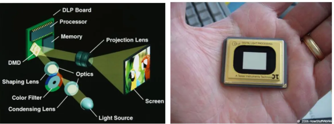
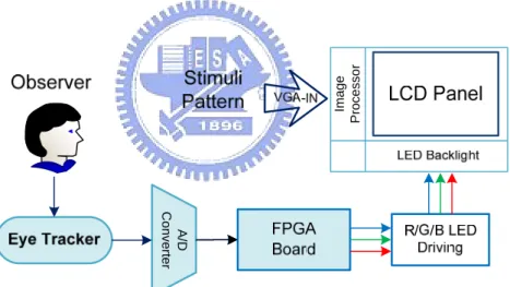
(16) 1.2 Field Sequential Display The field sequential display synthesizes colors in the time domain. By quickly flashing the red, green, and blue field one after the other, the observer is unable to distinguish the time difference between the three channels in Figure 1.. Figure 1: Field sequential display separates RGB fields.. The field sequential technology has been successfully used in TI’s DLP-based projectors, which use fast-switching micro mirrors to produce gray-levels and a color wheel to produce the primaries as shown in Figure 2. In this way, resources can be shared by the three channels and hardware cost can be greatly reduced. If such technology can be adapted for the LCD (i.e., FSC-LCD), not only its luminance efficiency can be increased to 3X, which equates to considerable power savings, but also the hardware cost can be cut down to 80% because the costly color filter process on the glass substrate can be eliminated. Unfortunately, unlike DLP, the slow response time of liquid crystals limits the highest frame rate of field sequential LCD and results in severe color breakup artifacts. Due to its nature of synthesizing colors temporally, FSC-LCD suffers from the color breakup phenomenon when eye movement and stimulus movement are out of sync. When the red, green, and blue components of the same stimulus project onto different locations of observer’s retina, color breakup is bound to happen depending on stimulus and 3.

(17) viewing conditions.. Figure 2: How DLP projection works and Digital Micro-mirror Device (DMD) chip.. Nevertheless, the field sequential LCD has the advantage of flexible backlighting schemes. The LED backlights are capable of generating arbitrary waveform for each of the three primaries or their combinations in arbitrary order [1].. 1.3 Color Breakup The most infamous artifact on field sequential displays, the color breakup phenomenon (CBU) shown in Figure 3, occurs when the red, green, and blue components of the same object project onto different locations of retina upon eye movement. Originated in the 80s, the study of field sequential display revived in the recent years for the temptation of high optical efficiency, high spatial resolution, and low manufacturing cost to the liquid crystal display technology (LCD) [2][3]. Suffering from slow response time, LCD is prone to the CBU artifacts. Despite its long research history, the foundation of CBU is still difficult to analyze due to the tangling causing factors such as the target movement, eye movement, field rate, target luminance, target pattern, primary colors/waveforms, ambient light, eccentric angle, viewing conditions, etc. [4].. 4.

(18) Figure 3 : Motion-induced the color breakup in field sequential display.. 1.4 Organization In this thesis, three approaches are proposed for minimizing display artifacts which are induced by eye movement. From slow to fast, these artifacts are: viewing angle-dependent color shift caused by head movement, color breakup caused by smoothly pursued eye movement, and color breakup caused by saccadic eye movement. A platform for evaluating perceivable color breakup of human eye is proposed in Chapter 2. In Chapter 3, for saccadic color breakup, a custom-made electro-oculogram circuit is used to detect the events of saccadic eye movement. In Chapter 4, for pursued color breakup, an eye-tracker is used to detect the gaze velocity such that the image chroma can be reduced for suppressing color breakup at run-time. In Chapter 5, for viewing angle-dependent color shift, an infrared sensing mechanism is used to detect the head position. The LCD panel transmittance and backlights are modulated to compensate for the color shift accordingly. Finally the conclusions and the future works are given.. 5.

(19) Chapter 2 Color Breakup Phenomenon Color Breakup Phenomenon 2.1 Measuring Pursued Color Breakup Due to its nature of synthesizing colors temporally, the field-sequential-color liquid-crystal-display (FSC-LCD) suffers from color breakup phenomenon when eye movement and stimulus movement are out of sync. When the red, green, and blue components of the same stimulus project onto different locations of the observer’s retina, color breakup is bound to happen depending on stimulus and viewing conditions. Therefore, a robust model of predicting color breakup is demanded by designers of field sequential displays. To derive such a model, statistical data must be collected from subjective experiments with human subjects. However, color breakup is a spontaneous phenomenon, which is very difficult for untrained human subjects to judge its existence. Therefore, more than just subjective experiments, carefully designed psychophysical experiments are required to collect sound experimental data and derive accurate color breakup prediction models. In literature, the CBU-related studies can be categorized as follows. (a) Analytical method: The moving target is mathematically modeled by its colorimetric parameters and moving velocity [5]. Assuming perfectly pursuing eye movement, the perceived CBU is predicted by Grassman’s law of additive color, which unfortunately does not hold under eye movement, as shown in Figure 4.. 6.

(20) Figure 4: (a) An ideal light emission patterns (not possible to realize). (b) Perceived original image. (c) Actual light emission patterns with positive and negative equalizing pulses. (d) Resultant perceived image [5].. (b) Photonic measurement: High-speed cameras are used to emulate the eye movement and to capture the process of colors falling apart [6]. Such experiments build the basis of photometry-based analysis, which however is still discrepant from the visually perceived artifacts, as shown in Figure 5.. 7.

(21) Figure 5: The target image ran at the 10° saccade. Initial and end views are marked with dashed rectangles [6].. (c) Subjective measurement: Commonly used in subjective experiments is a white box moving linearly on black background to provoke the worst CBU. The task of human subjects is to judge if any chromatic strips perceived on the edges [7]. In our experience such setup fails to reproduce reliable data because (i) perfectly pursuing the linear target movement on small displays is difficult and results in different degrees of CBU, and (ii) focusing on whether the edge is colored or not hinders us from considering the other important parameters such as stimulus size and spatial frequency as shown in Figure 6 and Figure 7.. Figure 6: The motion contrast measurement and analysis method [7]. 8.

(22) Figure 7: Two different color transitions used to judge CBU [7].. (d) Psychophysical measurement: The foundation of Color Science is based on psychophysics because even when judging color of still stimuli the bios of human subjects can lead to significant variation. Thus, to accurately access the spontaneous CBU phenomenon, carefully designed psychophysical experiments are required, as shown in Figure 8 and Figure 9 [8].. Figure 8: Sequence of screen configurations for the saccade task. This is an illustration only – distances and sizes of objects on screen are not in correct proportions [8].. 9.

(23) Figure 9: Illustration of the white bar, with or without a yellow and red color edge, used in the sequential color task. The bars are not drawn to proportion. The color edges are shown in grayscale here, and are widened for easier viewing [8].. The goal of this chapter is to design an apparatus for assessing the detectability of color breakup for human subjects. Our psychophysical method is the Forced Choice method. In a forced choice experiment, two stimuli are presented and the human subjects have to pick the one with color breakup even if they cannot distinguish. In this way, the subjects’ preference of “detected”/”not detected” can be filtered out. We designed an experimental platform which can present stimuli with either sequential primaries or simultaneous primaries. In the sequential mode, which emulates a field sequential display, the red, green, and blue LED backlights are triggered one after the other with adjustable frequency, duty cycle, intensity, and order. In this mode, perceiving color breakup is possible. In contrast, in the simultaneous mode, which emulates a conventional display, the backlights are triggered at the same time, so color breakup is impossible to be observed. In both modes, the triggering frequencies are the same, so they both have the same degree of flickering. The subjects will not be able to use flickering as cue to guess, so we can separate the artifacts in the chromaticity domain (color breakup) from the luminance domain (flicker).. 10.

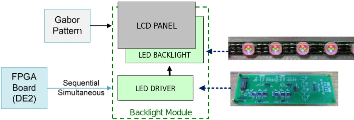
(24) The stimulus is a vertical grating pattern moving along a circle (Figure 10). Adjustable parameters include color, contrast, speed (angular velocity and radius), size, and spatial frequency [9][10].. Figure 10: Grating is clear at 3/9 but blur at 12/6 o’clock.. Compared with linear movement, our method has the following advantages: (1) Circular motion is easier to trace. Otherwise, when the subject fails to trace the moving pattern, severe color breakup will be perceived. (2) The vertical grating generates different spatial frequency – DC at 3 and 9 o’clock, and maximum at 12 and 6 o’clock. Therefore, the subject is supposed to perceive different contrasts between 3/9 and 12/6 o’clock, and we can isolate spatial frequency from the other variables such as velocity or contrast. The hardware is partially based on the previous work in [11][12]. The architecture is reviewed as follows.. LCD PANEL LED CCFLBACKLIGHT BACKLIGHT. LED DRIVER INVERTER. Backlight Module. Figure 11: Block diagram of the proposed platform for measuring pursued color breakup.. 11.

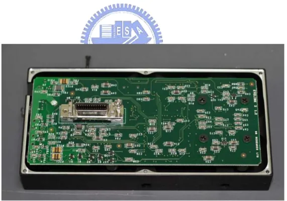
(25) A 19” TN-type LCD monitor (ViewSonic, VX912) was reworked for our purpose. Two lightbars, each with 24 LED chips, take place of the original CCFL backlights on the top and bottom edges of the panel. Three-in-one RGB LED chips (5WRGGB, Arima Optoelectronics Corporation) were used, as shown in Figure 12. To detour heat dissipation from the light-bar, the heat sink compound was applied to the gap between the thermal pads of LEDs and the lightbar, which attach to the metal frame tightly for better heat dissipation.. Figure 12: Close-up of LED chips with one red die, one blue die and two green dies and LED light-bar with 24 LED chips. For efficiency and stability, current mirror was chosen to drive the LEDs because it can supply stable constant electrical current and adapt to different forward voltages of each LED. It is suitable for driving LEDs because the output luminance is a function of the forward current through LEDs. A high constant current mirror (DD311, Silicon Touch Technology) was chosen as the LED driver because it can sustain up to one ampere forward current. It is a single-channel constant current LED driver incorporated current mirror and current switch. The maximum sink current is 100 times the input current value set by an external resistor or bias voltage. The maximum output voltage of thirty-three volts can provide more power to LEDs in series. The output enable (EN) pin allows dimming control or switching power applications. Based on the above mentioned thermal and charactictics, the maximum forwarding current of LEDs can be determined so that the reference current can be derived by divided by one hundred. The LEDs’ voltage supply VLED can be determined by calculating each LED’s VTH in series connection (Figure 13-17). 12.

(26) Figure 13: Current mirror for driving LEDs.. Figure 14: Layout of LED driver and lightbar.. Figure 15: Schematics of PCB design.. Figure 16: The final PCB.. 13.

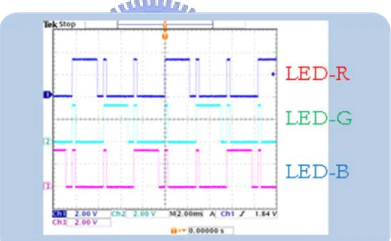
(27) Figure 17: The spectra of RGB LED backlights. Red, green, and blue LEDs have peaks at 631nm, 535nm, and 460nm, respectively.. To process the video signals, we used the Altera Development and Education board (DE2, Terasic), which is based on the Cyclone II 2C35 FPGA. The on-board TV decoder (ADV7181B, Analog Devices) was used to decode the input composite video signals into YCrCb format. We modified the factory sample Verilog codes to manipulate images and perform desired image processing. The results were output by a digital-to-analog converter (ADV 7123, Analog Devices) to generate the 640x480 VGA signals. We also used the FPGA to control the backlighting patterns. The control signals were outputted from the GPIO interface to trigger the LED drivers. Pulse-width-modulation was used to adjust the backlight intensity. To generate the stimuli, we used the Psychtoolbox, a Matlab-based library of handy functions for visual experiments [13]. It provides a simple interface to the high-performance, low-level OpenGL graphics library. To study color breakup under smooth-pursuing eye movement, our Matlab program is capable of generating moving Gabor patterns at different velocity, contrast, color, spatial frequency, and central/para-fovea area.. 14.

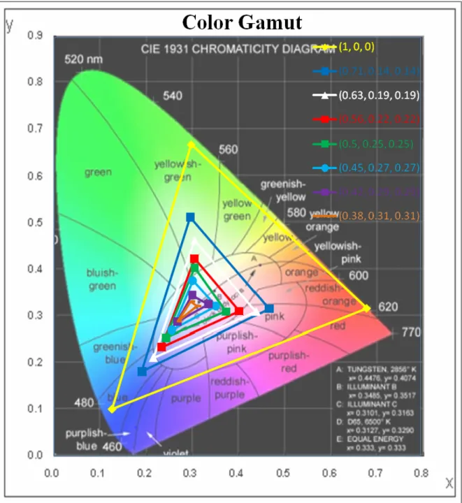
(28) 2.2 Gamut Reduction via Mixing Primaries In this work, the color breakup is suppressed by reducing the color gamut. The color gamut is reduced by mixing the red, green, and blue LED backlights. When each primary is mixed with the other two, its chroma is reduced such that the gamut size is reduced accordingly [14].. 2.2.1 Characterization of Primary Mixing On the experimental platform, each of the red, green, and blue LED backlights is triggered by an individual function generator. The triggering patterns are time-modulated as shown in Figure 18. The intensity of each primary is controlled by its duty cycle.. Figure 18: This is LED-R/G/B duty cycle waveform to adaptive gamut. To maintain the fixed luminance, the ratio between three primaries is limited by the form of (Red, Green, Blue) = (α, (1-α)/2, (1-α)/2).. (2-1). For example, before reducing the gamut size, the percentage of Red α, is 100%, while Green and Blue are both 0%. If the Redαis reduced to 80%, then Green and Blue are both reduced to (100%-80%)/2 = 10%. 15.

(29) The reduced gamut was measured by a colorimeter (CS-200, Minolta). The measured color coordinates are listed as follows Table 2-4. Table 2: Primary Red mixed with Green and Blue α, β, γ (1.00, 0.00, 0.00) (0.71, 0.14, 0.14) (0.63, 0.19, 0.19) (0.56, 0.22, 0.22) (0.50, 0.25, 0.25) (0.45, 0.27, 0.27) (0.42, 0.29, 0.29) (0.38, 0.31, 0.31). xR, yR (0.68, 0.32) (0.47, 0.32) (0.44, 0.31) (0.41, 0.31) (0.38, 0.31) (0.35, 0.32) (0.34, 0.33) (0.31, 0.32). Table 3: Primary Green mixed with Red and Blue α, β, γ (0.00, 1.00, 0.00) (0.14, 0.71, 0.14) (0.19, 0.63, 0.19) (0.22, 0.56, 0.22) (0.25, 0.50, 0.25) (0.27, 0.45, 0.27) (0.29, 0.42, 0.29) (0.31, 0.38, 0.31). xG, yG (0.30, 0.67) (0.30, 0.51) (0.31, 0.46) (0.31, 0.42) (0.31, 0.41) (0.30, 0.38) (0.30, 0.35) (0.30, 0.33). Table 4: Primary Blue mixed with Red and Green α, β, γ (0.00, 0.00, 1.00) (0.14, 0.14, 0.71) (0.19, 0.19, 0.63) (0.22, 0.22, 0.56) (0.25, 0.25, 0.50) (0.27, 0.27, 0.45) (0.29, 0.29, 0.42) (0.31, 0.31, 0.38). xB, yB (0.13, 1.00) (0.19, 0.18) (0.22, 0.21) (0.24, 0.23) (0.24, 0.25) (0.26, 0.27) (0.27, 0.29) (0.27, 0.29). 16.

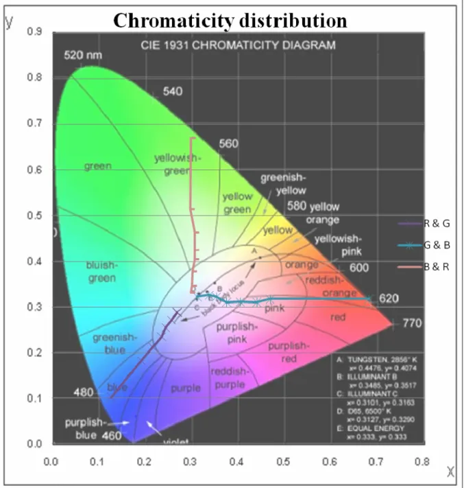
(30) The color coordinates are plotted on a CIEXYZ chromaticity diagram in Figure 19.. Figure 19: Saturation-reduced primaries. From outside to inside, the α ratio is 100%, 38%, 42%, 45%, 50%, 56%, 63%, and 71%, respectively.. 17.

(31) The reduced gamut sizes are shown in Figure 20.. Figure 20: Reduced gamuts. From outside to inside, the α ratio is 100%, 38%, 42%, 45%, 50%, 56%, 63%, and 71%, respectively.. 18.

(32) 2.3 Gamut Controller The gamut reduction is controlled by an FPGA board (DE2, Terasic), which controls the backlight driving patterns. The FPGA is programmed in Verilog. The ratio of gamut reduction is determined by the gaze velocity, which will be described in Chapter 3.. 19.

(33) Chapter 3 Suppressing Pursued Color Breakup with Eye-Tracking Suppressing Pursued Color Breakup with Eye-Tracking This chapter presents a contingent display (Figure 21) that suppresses the color breakup artifacts by using an eyetracker. Since color breakup is caused by eye movement only, we propose an adaptive system, which has dual modes. In Normal mode, when eye movement is absent, no adjustment is required. In Suppressed mode, when eye movement is detected, the display color is adjusted to minimize color breakup. The eye movement, i.e., gaze position, is. Image Processor. detected by an eyetracker.. A/D Converter. Figure 21: Block diagram of a contingent display system.. Figure 21 shows the block diagram of the proposed system. The FPGA was programmed in Verilog to calculate the velocity of eye movement, i.e. gaze velocity, and to control the color gamut. The color breakup is minimized by dynamically reducing the color gamut, which is done by mixing the red, green, and blue primaries. The ratio of reduced color gamut depends on the gaze velocity. Because the color gamut is reduced only when eye movement occurs, color quality will not be compromised when eye movement is absent. 20.

(34) 3.1 Introduction to Eye-Tracking Eyetracker can be implemented by different sensing techniques. This chapter focuses on the video-based eye tracking. Another technique will be investigated in the following chapter. A typical video-based eyetracker consists of a high-speed camera, infrared illuminators, a high-speed frame grabber, and an FPGA-based image processor. We used an SR EyeLink 1000 (SR Research Ltd., Mississauga, Ontario, Canada) eyetracker to acquire the gaze position at a sampling rate of 1000 Hz, which was transferred to the FPGA board via an A/D converter. This video-based eyetracker uses a high-speed CCD sensor to track the right or left eye and produces images at a sampling rate of 1000Hz. The EyeLink 1000 is used with a host PC running on DOS (Figure 22). The eyetracker is used with a PC with dedicated hardware for doing the image processing necessary to determine gaze position. Pupil position is tracked by an algorithm similar to a centroid calculation. Measuring eye movements during psychophysical tasks and experiments is important for studying eye movement control, gaining information about a level of behavior generally inaccessible to conscious introspection, examining information processing strategies, as well as controlling task performance during experiments that demand fixation or otherwise require precise knowledge of a subject’s gaze direction. Eye movement recording is becoming a standard part of psychophysical experimentation. Although eye-tracking techniques exist that rely on measuring electrical potentials generated by the moving eye (electro-oculography, EOG) or a metal coil in a magnetic field, such methods are relatively cumbersome and uncomfortable for the subject [13].. 21.

(35) Figure 22: The EyeLink 1000 eyetracker [15].. High-performance video-based eyetrackers are available in market and widely used in the fields of psychology, design, and marketing. A new generation of eyetrackers is based on the non-invasiverecording of images of a subject’ eye using infrared sensitive video technology and relying on software processing to determine the position of the subject’s eyes relative to the head [13].. 22.

(36) The video data is captured by a high-speed camera, which is connected to a digital frame grabber in the host computer uses. These components will be described as follows. In front of the lens, an infrared filter (093 30.5mm, B+W) is used to filter the infrared band. There is also a 30.5mm rubber hood to prevent glare in Figure 23.. Figure 23: The optical components of eyetracker.. A CCTV lens (23FM25SP, Tamron) is used for the 2/3” CCD sensor. It has a focal length of 25mm, 1:1.4 aperture, 1.3 megapixel and C-mount connector as shown in Figure 24.. Figure 24: The Tamron 23FM25SP lens .. 23.

(37) Figure 25: The high-speed CCD sensor -- front view.. Figure 26: The high-speed camera module -- rear view.. 24.

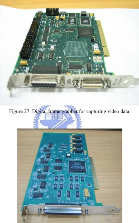
(38) A digital frame grabber (Pheonix AS-PHX-D24CL-PCI32, Active Silicon) is used for capturing the video data at 40MHz via 32-bit 33MHz PCI, as shown in Figure 27.. Figure 27: Digital frame grabber for capturing video data.. Figure 28: Analog interface card for external communication.. 25.

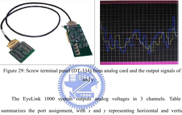
(39) The host PC performs real-time eye tracking, while computing eye gaze position on the subject display. On-line detection analysis of eye-motion events such as saccades and fixations are also performed. The EyeLink 1000 system supports analog output and digital inputs and outputs via the screw terminal panel of the DT334 and analog card to do data transformation, as in Figure 28-23.. Figure 29: Screw terminal panel (DT-334) from analog card and the output signals of x and y.. The EyeLink 1000 system outputs analog voltages in 3 channels. Table 5 summarizes the port assignment, with x and y representing horizontal and vertical position data, and P representing pupil size data. Table 5: Analog data output assignments of DT334 Eye tracking mode. Analog Output Mapping. DAC0 Pin28 O/P Pin27 Rtn. DAC1 Pin62 O/P Pin61 Rtn. DAC2 Pin30 O/P Pin29 Rtn. Left / Right. Monocular. x. y. P. Here, we briefly introduce the experimental operation and settings with eyetracker. It records gaze position and setups procedure included as the setup camera, calibrate, validate, and output record for running an experiment. We could afford supports offline analysis. The following Figure 30 shows the flow of the control software of the host PC. 26.

(40) Figure 30: EyeLink 1000 tracker application navigation.. The EyeLink 1000 system ensures its reliability from the performance. It supports the following features: . The Off-line mode is the default start-up screen for EyeLink 1000.. . The Setup Camera screen is the central screen for most EyeLink 1000 setup functions.. . Calibration is used to collect fixations on target points, in order to map raw eye data to gaze position data.. . The Output screen is used to manually track and record eye movement data.. . The Validate screen displays target positions to the participant and measures the difference between the computed fixation position and the fixation position for the target obtained during calibration.. . The Set options screen allows many EyeLink 1000 tracker options to be configured manually.. . The Record screen does the actual data collection.. . The Drift Correct screen displays a single target to the participant and then 27.

(41) measures the difference between the computed fixation position during calibration and the current target. The other details can be found in [15]. In this work, we needed to use the stand-alone mode and preset functions including calibration, validate, mouse simulation, and output record of the eyetracker. The gaze positions acquired by the eyetracker are transferred to the FPGA board via an A/D converter. The next section will describe the circuit, interface and functionality of the A/D converter.. 3.2 Interfacing the Eyetracker – Analog to Digital Converter We built the hardware interface for receiving gaze position from the eyetracker in real time. The target eyetracker is an EyeLink 1000 (SR Research Ltd., Mississauga, Ontario, Canada), which provides only analog signals of gaze position. We designed an analog-to-digital (A/D) converter to receive the real-time gaze positions. We programmed an FPGA board to calculate and analyze the gaze velocity. We used an A/D converter which supports 12-bit resolution (AD1674, Analog Devices) [16]. The block diagram is shown in Figure 31.. 28.

(42) Figure 31: AD1674 function block diagram.. Based on the AC characteristics of the AD1674 specification (Figure 32), it operates in the stand-alone mode, which converts the gaze positions from analog signals to encode the digital signal for the FPGA. The block diagram of hardware design shows in Figure 33. The R / C pin description is active high for a read operation and active low for a convert operation. The FPGA board can display gaze position (Ex, Ey) on its 7-segment displays.. Figure 32: Stand-alone mode Timing both low and high pulse for an R / C pin. 29.

(43) FPGA board. AD1674 x2. Eyetrack – gaze position. (Ex, Ey). Ex:DB[0:11]. I/O1[0:11]. Ey:DB[12:23]. I/O1[12:23] I/O1[34]. X: R / C. Ex and Ey show on 7-segment display. I/O1[35]. Y: R / C. Figure 33: Block diagram of hardware design.. The dual channel 12-bit A/D converter circuit was drew and implemented for converting analog signals of gaze position as shown in Figure 34 and Figure 35. ADC Used to Stand-Alone Mode GPIO_1-B[0:23] -15V. U1 AD1674. X-R/C. 8. R5. 14. REF OUT. DB7 DB6 DB5 DB4. REF IN. DB3 DB2 DB1 DB0. 20Vin. 2 3 4 6 5. 27 26 25 24. GPIO_1-B11 GPIO_1-B10 GPIO_1-B9 GPIO_1-B8. 23 22 21 20. GPIO_1-B7 GPIO_1-B6 GPIO_1-B5 GPIO_1-B4. 19 18 17 16. GPIO_1-B3 GPIO_1-B2 GPIO_1-B1 GPIO_1-B0. 1K. Y-R/C. 8 R4 R6. Vee. 12/8 CS A0 CE R/C. STS. 12 14. J1 GPIO_1-B0 GPIO_1-B2 GPIO_1-B4 GPIO_1-B6 GPIO_1-B8 GPIO_1-B10 GPIO_1-B12 GPIO_1-B14 GPIO_1-B16 GPIO_1-B18 GPIO_1-B20 GPIO_1-B22. +3.3V. X-R/C. 1 3 5 7 9 11 13 15 17 19 21 23 25 27 29 31 33 35 37 39. DB11 DB10 DB9 DB8. REF OUT. DB7 DB6 DB5 DB4. REF IN. 49.9. Y POSITION SIGNAL. +5V. Vlogic Vcc. 49.9 10. 10Vin AGND. 13. BIP OFF. 9. X POSITION SIGNAL. DB11 DB10 DB9 DB8. 49.9 12. 28 R2. 49.9 10. 1 7. DGND. R3. STS. 12/8 CS A0 CE R/C. U2 AD1674. 11. 13. BIP OFF DB3 DB2 DB1 DB0. 20Vin. 11 28. 27 26 25 24. GPIO_1-B23 GPIO_1-B22 GPIO_1-B21 GPIO_1-B20. 23 22 21 20. GPIO_1-B19 GPIO_1-B18 GPIO_1-B17 GPIO_1-B16. 19 18 17 16. GPIO_1-B15 GPIO_1-B14 GPIO_1-B13 GPIO_1-B12. 10Vin AGND. 1K. Vee. 15. R1. 2 3 4 6 5. C2 0.1uF. +5V. Vlogic Vcc. 9. 1 7. -15V. 15. C1 0.1uF. +5V. +15V +5V. DGND. +15V +5V. GPIO_1 2 4 6 8 10 12 14 16 18 20 22 24 26 28 30 32 34 36 38 40. GPIO_1-B1 GPIO_1-B3 GPIO_1-B5 GPIO_1-B7 GPIO_1-B9 GPIO_1-B11 GPIO_1-B13 GPIO_1-B15 GPIO_1-B17 GPIO_1-B19 GPIO_1-B21 GPIO_1-B23. GPIO_1-B[0:23]. Y-R/C. Figure 34: Dual channel 12-bit A/D converter schematic.. 30.

(44) Figure 35: A/D converter implementation.. 3.3 Experimental Platform At beginning, we generated a moving target with constant speed on display and asked subject to trace the target movement. To generate the stimuli, we used the Psychtoolbox, a Matlab-based library of handy functions for visual experiments. It provides a simple interface to the high-performance, low-level OpenGL graphics library. To study color breakup under smooth-pursuing. eye movement, our Matlab program is capable of generating moving. Gabor patterns at different velocity, contrast, color, spatial frequency, and central/para-fovea area. At the same time, we used an eye tracker to record the eye movement and then calibrated the FPGA results. At the end, the velocity is shown on the LED bar for debugging purpose. The correlation between gaze velocity and LED index is shown in this chart. The faster the eye moves, the more LEDs turn on. Such analog indicator is very convenient for us to run visual experiments, as shown in Figure 36.. 31.

(45) Stimuli: Image source input by Matlab’s Psychotoolbox. A circle moving: Adjust velocity. Display. Observer: Answer “Yes” or “No” CBU. 1m. Eyetracker system. (Ex, Ey). A/D converter. Result: FPGA board LED index. Figure 36: Experimental platform system.. The stimulus generated by Matlab and the Psychotoolbox function is a vertical grating pattern moving along a circle. Adjustable parameters include color, contrast, speed (angular velocity and radius), size, and spatial frequency.. 3.4 Gaze Velocity Analyzer We used an FPGA/Verilog to analyze the gaze velocity. First, it samples the raw data of gaze position (Ex, Ey) from the custom-made A/D convertor attached to the eyetracker. In the Verilog code, the displacement (Δx2+Δy2) is calculated. Since eye movement is very fast, a low-pass filter is required, which was done by using moving average. We then used the Psychtoolbox to generate a target moving on a circle at constant rate. Human subjects were required to activate the eyetracker. The subjects were asked to trace the target closely. The data from the eyetracker were recorded for later analysis.. 32.

(46) By regression analysis, we obtained the mapping between the pixel velocity (on the two-dimensional display) and the actual gaze velocity (in the three-dimensional space). The data were reported in the following Table 6. Table 6: Experiment result for evaluating relationship between gaze velocity and LED index Velocity oiv by (cm/sec) E.T.. LED index. Times. Run 1. Run 2. Run 3. Run 4. Average. 1cycle second. rad/sec. 5. 80. 6.7. 6.7. 6.7. 6.8. 6.8. 1.4. 4.7. 98.8. 4. 100. 8.4. 8.5. 8.4. 8.5. 8.5. 1.7. 3.7. 79.0. 3. 130. 11.0. 11.0. 11.0. 10.9. 11.0. 2.2. 2.9. 60.9. 2. 190. 16.1. 16.0. 15.8. 15.9. 15.9. 3.2. 2.0. 41.9. 1. 400. 33.6. 33.5. 33.4. 33.4. 33.5. 6.7. 0.9. 20.0. 280 200 130 70 20. For the purposes of debugging and demonstration, the gaze velocity was shown on the FPGA board by using the LED bars. The following chart shows the relation between the gaze velocity and LED indicator, as shown in Figure 37.. Figure 37: The linear correlation between LED index and gaze velocity.. 33.

(47) For example, in Figure 38, the two lit LEDs shown in the left picture represent a slower eye movement, while the 7 lit LEDs on the right show a faster one. The velocity of last saccade remains on the 7-segment display.. Figure 38: The velocity of eye movement is indicated by the number of lit LEDs.. 3.5 Summary We have implemented an eyetracker-based interactive display system. It used FPGA board with Verilog code to calculate velocity of eye movement. We built the hardware interface for receiving gaze position from the eyetracker in real time. We programmed an FPGA board to analyze the gaze velocity. Because the gaze velocity is an important parameter for the following psychophysical experiment, we have to identify the gaze velocity. We calibrated very carefully so we successfully obtained a linear correlation as shown on the chart. It is quite convenient for us to identify the gaze velocity with the LED-index while undertaking the psychophysical experiment. The human visual action is changing immediate, gaze velocity move a viability of relies on eye movement and update rate is very fast on the 7-segment display.. 34.

(48) Chapter 4 Suppressing Saccadic Color Breakup with Electro-Oculogram Suppressing Saccadic Color Breakup with Electro-Oculogram Electrooculography (EOG) is a technique for measuring the resting potential of the retina. The resulting signal is called the electrooculogram. Typically the EOG is used in ophthalmological diagnosis and in recording eye movements. In the application of eye movement measurement, pairs of electrodes are placed either above and below the eye or to the left and right of the eye. If the eye is moved from the center position towards one electrode, this electrode detects the positive side of the retina and the opposite electrode detects the negative side of the retina. Consequently, a potential difference occurs between the electrodes. Assuming that the resting potential is constant, the recorded potential is a measure for the eye position [17][18][19].. Figure 39: The potential difference generated by eye movement.. 35.

(49) In this chapter, we describe an interactive display system that suppresses color breakup by detecting saccadic eye movement with EOG. First, the design and implementation of EOG are described in Section 4.1. To evaluate the EOG accuracy and performance, the methods and results are presented in Section 4.2. Section 4.3 depicts how to incorporate the EOG circuit in an interactive display system.. 4.1 Circuit Design of EOG The kernel of an EOG circuit is a high-quality amplifier. Our EOG design consists of the following five stages: an instrument amplifier, a 10Hz low-pass filter, a 2Hz high-pass filter, a notch filter, and a gain amplifier. Figure 40 shows the block diagram.. Output. Electrodes. Figure 40: Block diagram of our EOG circuit.. 4.1.1 Stage I: Instrument Amplifier An instrument amplifier consists of two stages as illustrated in Figure 41. The first stage includes two op amplifiers (U1A and U2A) while the second stage has one (U3A). Such three-op-amp design is frequently called an instrument amplifier, which has the features of high input impedance, high CMRR, and high gain.. 36.

(50) Stage1 4 3. V1. Stage2 V+. + U1A OUT. 2. - 11. R4. 1. V-. R3. R2 R1. 11. 2. V2. - 11. OUT. 1. Vo. V-. V-. -. R4 U2A OUT. 3. V+. + U3A. R3 R2. 2. 4 3. + 4. 1. 0. V+. Figure 41: A sample circuit of an instrumentation amplifier.. The differential voltage gain of an instrumentation amplifier is. Ad =. R Vo =− 4 (V1 − V2 ) R3. ⎛ 2 R2 ⋅ ⎜⎜1 + R1 ⎝. ⎞ ⎟⎟ ⎠. (4-1). High-precision instrument amplifiers are commonly available nowadays. In our work, an instrument amplifier IC (AD620A, Analog Devices) was used (Figure 42).. Figure 42: Internal circuit of AD620A [20]. The AD620A’s gain is the resistor programmed by. 37.

(51) RG =. 19.4 KΩ , G −1. (4-2). where G is the differential voltage gain of AD620A.. 4.1.2. Stage II: Twin-T Band-Rejection (Notch) Filter. Figure 43 shows the second stage. A notch filter that passes all frequencies except those in a stop band centered on a certain frequency. A high-Q (filter quality) notch filter can eliminate a single frequency or narrow band of frequencies such as a band reject filter. In our EOG application, the main purpose of this notch filter is to reject the 60Hz AC noise from the power line. R1. R2. 27K. 27K C3 0.2uF. In. 0. V1 1Vac 0Vdc. Out V. C1. C2. 0.1uF. 0.1uF. 0. R3 13.5K. 0. Figure 43: Circuit of the notch filter.. 38. Out.

(52) The DC gain of the notch frequency is given by. ADC = ( R1 + R2 ) / R1.. (4-3). The notch frequency is. fc =. 1 2π ⋅ R1 ⋅ C1. (4-4). To set f c ≒ 60 Hz, we chose R1 = 27K ohm, and C1= 0.1uF. PSpice was used to simulate the frequency response of our design of the notch filter. The result is shown in Figure 44. 1.0V. 0.8V. 0.6V. 0.4V. 0.2V. 63.096 0V 1.0Hz V(OUT). 3.0Hz. 10Hz. 30Hz. 100Hz. 300Hz. 1.0KHz. Frequency. Figure 44: Frequency response of the notch filter circuit simulated by PSpice.. 39.

(53) 4.1.3. Stage III: High-Pass Filter. The third stage is a high-pass active filter for attenuating the low-frequency noise while passing the higher frequencies. Figure 45 shows our design, a Bessel type filter and Sallen-Key filter configuration. The second-order equation of the high-pass filter is. Vo =. S2 ⎡ 1 1 ⎤ 1 S + S⎢ + ⎥+ ⎣ R1C1 R1C 2 ⎦ R1 R2 C1C 2. ⋅ Vin. (4-5). 2. ,. where S = jω .. Vee -5v. R1. 0. 1.8M Vcc. 0 C1. C2. 0.1uF. 0.1uF. in. + R2 1.8M. Vin. 0. 0. V+. Vcc +5v. Vee. OUT -. out. V-. Vcc. Vee. Figure 45: The high-pass filter circuit design.. 40. Out.

(54) PSpice-simulated frequency response of the high-pass filter circuit is shown in Figure 46. 1.0V. 0.8V. 0.6V. 0.4V 1.0Hz V(OUT). 3.0Hz. 10Hz. 30Hz. 100Hz. Frequency. Figure 46: Frequency response of the high-pass filter.. 4.1.4. Stage IV: Low-Pass Filter. Figure 47 shows the fourth stage, a unity-gain Sallen-Key low-pass active filter for attenuating the high-frequency noise. The low-pass filter is Butterworth type and in the Sallen-Key configuration. The frequency response of low-pass filter is shown in Figure 48.. Vee -5v. C2 0.1uF. 0. Vcc. 0 R1. R2. 85K. 85K. in. +. OUT. C1 Vin 0.1uF. 0. 0. V+. Vcc +5v. Vee. -. out. V-. Vcc. Vee. Figure 47: The low-pass filter circuit design. 41. Out.

(55) 1.0V. 0.5V. 0V 1.0Hz V(OUT). 3.0Hz. 10Hz. 30Hz. 100Hz. Frequency. Figure 48: Frequency response of the low-pass filter circuit.. It uses a few passive components to function as a second-order low-pass filter while reducing signal noise. The second-order equation is. 1 R1 R2C1C 2 Vo = ⋅ Vin, ⎡ ⎤ 1 1 1 S2 + S⎢ + ⎥+ ⎣ R2 C 2 R1C 2 ⎦ R1 R2C1C 2. where S = jω .. 42. (4-6).

(56) 4.1.5. Stage V: Gain Op Amplifier. Figure 49 shows the final stage, an inverting amplifier circuit. The output voltage is. Vo = −. R2 Vi R1. (4-7). R2. R1 OUT. Vi. Vo. +. 0. 0. Figure 49: A typical design of inverting amplifier circuit design. It gives the output voltage in terms of the input voltage and the two resistors in the circuit. This is a basic operational amplifier schematic for general purpose.. 4.1.6 Prototype After putting the five stages together, the prototype is shown in Figure 50. The EOG circuit design shows in Figure 52.. Figure 50: Prototype of the EOG circuit. 43.

(57) The EOG circuit requires a pair of input supply voltages (+5V and -5V) to operate. A pair of electrodes is placed around the left and right of the eyes, and an indifferent electrode is placed on the wrist, as shown Figure 51. It is necessary to clean the skin before attaching the electrodes. Oil and dead skin degrade the quality of output signals.. Figure 51: Connecting the EOG electrodes to human body.. 44.

(58) Figure 52: EOG schematics. 45.

(59) The initial test showed that the EOG circuit function correctly, as shown in Figure 53-55. The following pictures show the connection between subject’s eye movement and the EOG output spikes. The next task is to find the relation between EOG output and eye movement.. Figure 53: A right-bound saccade causes a negative spike on EOG.. Figure 54: Fixation causes nothing on EOG.. 46.

(60) Figure 55: A left-bound saccade causes a postive spike on EOG.. 4.1.7 Calibrating the EOG Circuit We designed experiments to establish the relation between the input gaze-position of the observer and the output voltage of the EOG circuit. We asked the observer to generate a given amount of eye movement while recording the output voltage of the EOG circuit with an oscilloscope. Figure 56 shows the experiment setup. A series of markers was fixed on a horizontal line, which was placed one meter away from the subject. These markers are set for the observer to induce predefined saccadic eye movement. An audible beep was used to cue the observer to start the saccade.. 47.

(61) -30o. -15o. 0o. 15o. 30o. 1m. Observer Figure 56: Markers for the observer to induce predefined saccadic eye movement.. In Figure 57, the EOG output waveform (lower curve) was recorded by an oscilloscope along with a step pulse (upper curve), which triggers the audible beep.. Action. Action. Figure 57: Eye movement from 0° to -7.5° and from 0° to 7.5°.. 48.

(62) Action. Action. Figure 58: Eye movement from 0° to -15° and from 0° to 15°.. Action. Action. Figure 59: Eye movement from 0° to -22.5° and from 0° to 22.5°.. Action. Action. Figure 60: Eye movement from 0° to -30° and from 0° to 30°.. 49.

(63) Based on these graphs, we can make the following quick observations: 1) The EOG is triggered by gaze velocity rather than gaze position. 2) The EOG signal can be used to detect saccades by filtering the high frequency component. A rapid change of gaze velocity indicates an event of saccadic eye movement. 3) Polarity of the EOG signal spike shows the direction of saccades. A positive spike indicates a left-to-right saccade. A negative spike indicates a right-to-left saccade. 4) The amplitude of the EOG signal represents the amplitude or speed of saccades. We measured the output level of EOG circuit to record in different saccade amplitude, as the measurement data list in Table 7. Table 7: Measured EOG output for predefined saccades Saccade amplitude Left-bound saccade Saccade amplitude Right-bound saccade -7.5°. 440 mV. 7.5°. 560 mV. -15.0°. 760 mV. 15.0°. 960 mV. -22.5°. 1.04 V. 22.5°. 1.24 V. -30.0°. 1.44 V. 30.0°. 1.92 V. 50.

(64) The relationship between EOG and saccades is plotted in Figure 61.. Figure 61: EOG signal strength vs. amplitude of saccades.. 4.2 Accuracy Evaluation with Eyetracker We used two methods to evaluate the accuracy of our EOG circuit. The first method, eye tracking, is described in this section. The other method is covered in the next section. The same eyetracker, EyeLink 1000, described in Chapter 3 was used. We assume this eyetracker having 100% accuracy. Its detection results were used as the baseline to evaluate our EOG design. We used both eyetracker and EOG signal to record eye movement at the same time with the oscilloscope. The subject was asked to look at a movie around 100 seconds as shown in Figure 62. In order to analyze the performance of our EOG circuit, the accuracy that based on saccadic amplitude can be obtained by comparing the EOG signal with the eyetracker signal.. 51.

(65) Observe 1m. Eyetracker. Stimuli: Display a movie around 100 seconds. EOG Record by oscilloscope: 1.) Gaze position signal (Ex, Ey) 2.) EOG signal Figure 62: To record eye movement at the same time with eyetracker and EOG circuit.. During the experiments, both eyetracker and EOG are attached to the human subject to record eye movement at the same time. The following figure shows the output signals and the eyetracker and our EOG.. EOG. Eyetracker. Figure 63: (a) The upper line is the EOG signal. (b)The lower line is the eyetracker signal. The markers were detected saccades over the threshold amplitude.. 52.

(66) Since the eyetracker reports only the gaze position, to obtain the gaze velocity, the data needed to be analyzed offline, in which an algorithm for determining saccades was needed to obtain the curve in Figure 63. Next, a threshold needs to be determined. Any eye movement faster than the given threshold will be considered as a saccade. For example, in Figure 63, if the dash line is used as threshold, four right-bound saccades will be reported. After the analysis, two sets of detected events are obtained. Let S1 be the set of the saccadic events detected by the eyetracker. Let S2 be the set of the saccadic events detected by our EOG. The accuracy of our EOG can be determined by examining these two sets as shown in Figure 64.. S1: Eyetracker. S2: EOG. Miss Miss rate =S1-S2 =S1-S2. Hit = S1∩S2. False alarm =S2-S1. Figure 64: The intersection region is the hit rate of our EOG circuit. The left region is the miss rate. The right region is the false alarm rate. The hit rate, defined as the actual saccadic events detected by the EOG, is represented by the intersection of S1 and S2:. Hit rate = (S1 ∩ S2)/S1.. (4-8). 53.

(67) The miss rate, defined as the actual saccadic events but not detected by the EOG, is represented by the difference of S1 and S2:. Miss rate = (S1 - S2)/S1.. (4-9). The false alarm rate, defined as the non-saccadic events but reported by the EOG as saccades, is represented by the difference between S2 and S1:. False alarm rate = (S2 – S1)/S2.. (4-10). In the experiments, four human subjects were asked to watch a 100-second movie while their eye movements were recorded by the eyetracker and EOG simultaneously. The following Table 8 summarizes the experimental results. Table 8: EOG accuracy from 4 human subjects JW. WW. KL. ML. Avg.. Hit rate. 64.7%. 70.6%. 51.3%. 69.2%. 63.95%. Miss rate. 35.3%. 29.4%. 48.7%. 30.8%. 30.05%. False alarm. 17.5%. 7.7%. 16.7%. 10.0%. 9.05%. We conclude that our EOG circuit, in average, has a hit rate of 63.95%, a miss rate of 36.05%, and a false alarm rate of 9%. We consider it decent accuracy for an implementation costing less than NT $1,000. Note that the baseline eyetracker costs more than NT $2,200,000.. 54.

(68) 4.3 Accuracy Evaluation with EEG An electroencephalography (EEG) recorder (EGI 200 64-channel, EGI) was used to calibrate and verify our circuit implementation (Figure 65). EEG is the technique of measuring the electrical signals produced by the brain activities. The electrical potential is measure from the scalp with dozens of electrodes on a head-net. Usually 64, 128, or 256 electrodes are used at the same to detect and record the EEG signal at different locations in separated channels [21].. Figure 65: Components of EEG. (a) Channel map of a 64-channel sensor net. (b) 64-channel sensor net, medium size. (c) EEG Amplifier. (d) EEG and eyetracking recording at the same time.. 55.

(69) Among the 64 channels, we considered only the two channels near the ends of eyebrows (Figure 66, canthus) because they record the EOG signals that we need.. Figure 66: Only two channels across the eyes were used to record the EOG signals.. 56.

(70) The subjects were asked to perform predefined saccades between the markers fixed on an LCD TV, as shown in Figure 67.. Figure 67: Markers were placed every 4.8º for conducting amplitude-predefined saccades.. The recorded EOG signals were shown in Figure 68. Any horizontal eye movement causes changes on the two waveforms in opposite directions. A sharp spike indicates the occurrence of a saccade. We also observed that the larger the saccade, the taller the spike (e.g. the spikes within the red box). If a threshold is given (e.g. the horizontal dotted line), then the detected events of saccades can be determined. Therefore, by changing the threshold, the detection sensitivity for saccades can be controlled.. 57.

(71) Figure 68: EEG was used to calibrate and verify our EOG implementation.. The distance is 1m between the observer and screen. We made seven markers to divide partition on the display for eye target uses, as shown in Table 9. The in-between gaps on the screen are about 4.8º. Table 9: Saccade amplitude vs. EED signal Saccade amplitude. Spike height in EEG. (degree). signal (uV). 4.8. 0.54. 9.6. 2.01. 14.4. 3.60. 19.2. 3.64. 24.0. 3.81. 28.8. 7.27. 33.6. 7.30. 38.4. 7.52. 58.